Dynamic simulation tool for seismic analysis

(1)

Dynamic Simulation Tool for Seismic Analysis

by

Chun-Yi Wang B.S., Civil Engineering National Taiwan University, 1993

Submitted to the Department of Civil and Environmental Engineering in Partial Fulfillment of the Requirements for the Degree of

Master of Science in Civil and Environmental Engineering at the

Massachusetts Institute of Technology May 1998

@ 1998 Chun-Yi Wang

The author hereby grants to MIT permission to reproduce and to

distribute publicity paper and electronic copies of this theses document in whole or in part

Signature of Author ... ... ... ,... ... -. ... Department of Civil and Environm tal Engineering

May 8, 1998

Certified by ... .. ... ... ...Jonnor "Professor Jerome J. Connor Department of Civil and Environmental Engineering Thesis Supervisor

A ccepted by ... ...

Joseph M. Sussman Chairman, Department Committee on Graduate Students

(2)

Dynamic Simulation Tool for Seismic Analysis

by

Chun-Yi Wang

Submitted to the Department of Civil and Environmental Engineering May, 1998 in Partial Fulfillment of the

Requirements for the Degree of Master of Science in Civil and Environmental Engineering

ABSTRACT

Time history analysis of multi-degree-of-freedom structures subjected to general dynamic loading is a convenient and accurate way of representing the dynamic behavior of structures. It is widely used for determining the earthquake resistance in seismic engineering. However, the high computational requirement makes it difficult to implement by simple calculation. Thus, spectrum analysis and other simplified less accurate procedures are used instead of response history analysis. With the great improvement in personal computing capability in recent years, response history analysis with personal computers is now feasible. Furthermore, more complex and realistic problems such as non-proportional damping and highly damped structures can be handled. The thesis presents the mathematical formulation in state space that can handle a shear beam type of structure with arbitrary properties. The implementation of the mathematical formulation in a program named Motion Lab is described. This program provides a dynamic simulation environment for rapid prototyping and assessment of structural response. Key features are the graphical user interface and visual display tools for time history response. This program is intended to be used primarily as a learning tool for structural dynamics. It is also useful for preliminary structural design.

Thesis Supervisor: Dr. Jerome J. Connor

(3)

Acknowledgments

I would like to thank Professor Connor for giving me this chance to implement the

simulation environment. His guidance and encouragement inspired me throughout this thesis. I would also like to thank Joy for her great support, and my friends in MIT, who gave me help in both academics and daily life.

(4)

List of Tables

3.1 Requirement for Numerical Methods in the Analysis Procedure ... 33 5.1 Comparison between the results from convolution integral and Motion Lab ... 77 5.2 Comparison between the results from direct integration and Motion Lab ... 90

(7)

List of Figures

1.1 Functional Requirements and Corresponding Design Parameters of the Dynamic

Sim ulation Tool ... ... 11

2.1 Plot of k in complex plane ... 29

3.1 Procedure for the Analysis of General Dynamic Systems ... 32

3.2 Procedures for Finding Eigenvalues and Eigenvectors for nonsymmetric matrix 35 3.3 Elements of Upper Hessenberg Matrix ... 37

3.4 Data Ordering for an Eight-point Fourier Transformation ... 45

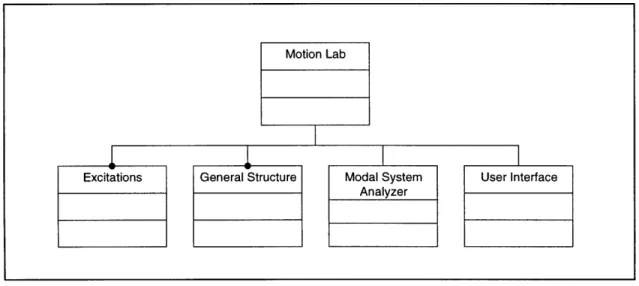
4.1 Static model for Motion Lab ... 54

4.2 Static model for the Excitation and General Structure ... 55

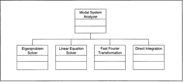
4.3 Static model for the Modal System Analyzer... 55

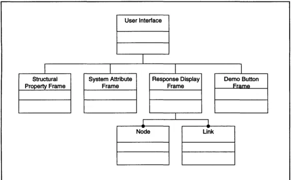
4.4 Static model for the User Interface ... 56

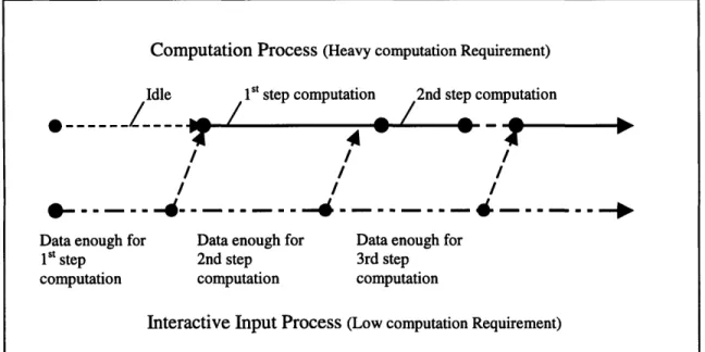
4.5 The idea of parallel computation for the input and computation process... 58

4.6 Precedence diagram of user interface and computation threads... 60

4.7 User interface of Motion Lab on Netscape browser... 62

4.8 System parameter setting dialog box ... ... 63

4.9 Mode/DOF attribute display panel... ... 65

4.10 Suggested operation of Motion Lab ... 68

5.1 The single-degree-of-freedom structure... ... 69

5.2 North-south component of El Centro earthquake... 71

5.3 Response plot of El Centro earthquake... 72

5.4 Setting up degrees of freedom of the structure... 73

5.5 System attribute setting ... 74

5.6 Select El Centro as the Excitation ... 74

5.7 Response plot from Motion Lab ... 75

5.8 Response demo at t=6.08sec... 75

5.9 Numerical Mode/DOF attribute form Motion Lab ... 76

5.10 Properties of the five-degree-of-freedom structure ... 77

5.11 El Centro response for the five-degree-of-freedom structure ... 82

5.12 Setting up the five-degree-of-freedom structure ... ... ... ... 83

5.13 Response plot of the five-degree-of-freedom structure ... 84

5.14 Numerical attribute of the first mode and DOF ... 85

5.15 Numerical attribute of the second mode and DOF ... 86

5.16 Numerical attribute of the third mode and DOF ... 87

5.17 Numerical attribute of the fourth mode and DOF... 88

(8)

Chapter 1 Introduction

1.1 Motivation

Matrix structural dynamic analysis is a complex procedure that involves many matrix operations and numerical computations. The extent of the complexity makes it difficult or even impossible to calculate by hand. Thus, the actual problem is either simplified to one that can be solved by simple computation or people have to resort to dynamic analysis program to get an accurate result. In the first case, the problem simplified may behaves far from the original system, thus it may not meet the accuracy requirement. On the other hand, spending hours to setup a dynamic analysis program such as ADINA or SAP is not efficient for people who mainly want to experiment with the structure and therefore need a simple setup procedure. For example, in the preliminary design phase, one needs a tool with simplified interface and good numerical accuracy that can be set up within minutes and return the result immediately. One needs to play around with several scenarios and have the feeling of the actual behavior of the structure within a limited amount of time.

Thus, a structural analysis tool that is simple to use and handles intensive computations is needed in two major areas. The first area is the preliminary earthquake design of structures for seismic excitation, the second area is mechanical vibration and structural dynamics education.

(9)

To understand how the tool may improve the preliminary design process, the traditional design procedure for earthquakes is examined. The procedure is divided into several steps. First, the structure is discretized into a lumped parameter system. Then the building code is introduced. From the properties of the structure and the seismicity of the region, the equivalent static lateral force each floor will take during earthquake is determined.

Most codes also permit dynamic analysis procedures of both response spectrum analysis (RSA) and response history analysis (RHA). The response history analysis calculates the time history of the structural response subjected to a given ground acceleration ii, (t). The response spectrum analysis computes the peak response of the structure during an

earthquake directly from the earthquake response spectrum.

The earthquake design procedures presented above can be improved in several aspects by applying the tool. First, the building earthquake design code can be verified or even substituted by the response calculated by the tool. The reason is that the code is only an approximation and a safety limit to normal structures; it does not take the property of the entire structure or the equivalent discretized structure into account. For example, only the fundamental frequency and maximum response properties from the design spectrum chart are considered to represent a structure and an earthquake impact. The same problem happens to the response spectrum analysis procedure. The structure peak response varies with the property of the structure, thus the effect of the summation of peak responses of several modes is not the real structural response because of the difference in phase lag

(10)

between modes. With the complete response analysis procedure built into a standard computing process, the preliminary design procedure can have a great support.

Other improvements can be made on the design procedure with the tool. First, the response of general structure with non-proportional damping can be evaluated. The state-space formulation works with complex modes and frequencies, and thus can deal with arbitrary damping In addition to accurately predicting the response of a highly damped structure, the influence of damping on the mode shapes and frequencies can be examined.

Secondly, several earthquake spectrums can be imposed on the structure to get a complete portrait of the response characteristics of the structure. For example, responses of the structure to different earthquakes with different frequency contents can be used to establish an improved estimate of the required rigidity.

The other application area of great potential is education. Textbooks on vibration analysis and structural dynamics give examples based on proportional damping, because real quantities are easier to comprehend and compute. However, non-proportional damping is generally used in buildings. With the help of this analysis tool, a more realistic treatment of the subject can be presented. Realistic studies of highly damped structures with non-proportional damping can be carried out.

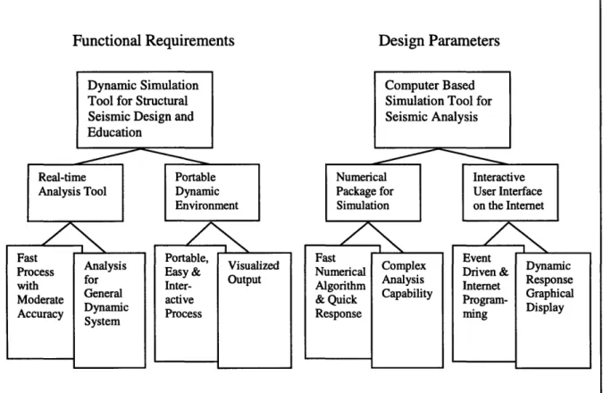
The main functional requirements and corresponding design parameters for the simulation environment are listed in Figure 1.1.

(11)

Figure 1.1 Functional Requirements and Corresponding Design Parameters of the Dynamic Simulation Tool

1.2 Review of Previous Work

Previous works related to the implementation of the simulation environment fall into two categories. One category is research on general formulation and numerical computation methods in structural dynamics. The other category is computer-aided design and education system for mechanics.

(12)

Research efforts on the application of state-space formulation to structural analysis are described in [1-3]. The capability of the state-space formulation in the dynamic analysis of structures has been proved. Also, the basic transformations between real and complex system have been derived.

On the other hand, two different types of software are developed for computer-aided design and education. The first are the tools for accurate structural analysis. Software systems such as ADINA, ANSYS and SAP are out of the scope of the thesis and will not be discussed. The other types of software for preliminary design and education are still focused on statics problem. Educational programs for the analysis of simple beams and trusses are developed in [4][5]. They are all portable on the internet and have a user friendly interface.

1.3 Organization of the Thesis

Comparing the functional requirements to the previous work, a more general structural dynamic simulation environment with easy to use interface and short responding time is needed. The following chapters discuss the underlying theories and the implementation of the proposed environment.

In the next chapter (Chapter 2), the fundamental state-space formulation is stated, and then an uncoupled version is derived by solving the associated eigenvalue problem.

(13)

Applying the uncoupled complex equations, responses for free and forced vibrations are generated. After that, modal properties and mode shapes of complex modes are discussed.

Chapter 3 describes the numerical algorithms used in dynamics analysis. A standard numerical procedure for obtaining the response of a general dynamic system is proposed. Then, the numerical algorithm for generating complex eigenvalues and eigenvectors of a general matrix is described. Both frequency domain analysis and direct integration method are discussed for complex modal analysis.

Chapter 4 focuses on the architecture and implementation of the environment. First, the design of the objects is discussed. Then, the strategy for optimizing the computations for dynamic simulation is proposed. Finally, the implementation and the operation of the system is described.

Chapter 5 discusses the evaluation and testing of the system. Several scenarios are provided. Interactive process between the program and user is presented. The eigensystems and response histories are also verified by several MATLAB programs.

(14)

Chapter 2 Fundamental Formulation for General Dynamic System

2.1 Introduction to State-space Formulation

The governing equations of motion for a multi-degree-of-freedom mechanical system are given by

M ii(t) + C u(t) + K u(t) = P(t) (2.1)

where M is the mass matrix, C is the damping matrix, and K is the stiffness matrix. Vectors u(t), A(t), and ii(t) are the displacement, velocity, and acceleration vectors of the degrees of freedom in the system. Vector P (t) is the external forcing function as a function of time t. If P (t) is zero at all time t and u(O), u(0) are given as initial conditions, (2.1) is often referred to as the free vibration problem. Otherwise, if P (t) is not zero, the problem is categorized as the forced vibration problem.

Equation 2.1 is recognized as a set of coupled second order differential equations. One solution strategy is based on applying a linear coordinate transformations to uncouple the equations. For the undamped (C = 0) and proportional damping1 cases, the uncoupled equations can be obtained easily by first solving first order eigenvalue problem for the

' If m ,~n are the mth and nth mode-shape vector of the undamped system, and if for the damping matrix C, the orthogonality holds, i.e., C On = 0 for all m # n, then C is called the proportional damping.

(15)

system, and using the mutually orthogonal eigenvectors as the basis functions for the coordinate transformation. Then, use the solution procedure for second order differential equation to solve each of the uncoupled equations separately.

However, when dealing with dynamic systems with non-proportional damping, orthogonal eigenvectors of the real system does not exist. The procedure for uncoupling the system with proportional damping is not valid. Thus, to obtain an uncoupled set of equations for the system, one has transform the system to state-space system to reduce the problem to a first order eigenvalue problem.

The transformation from the real system as shown in Equation 2.1 to the state-space formulation is performed by considering the velocity vector another unknown variable of the system. The vector composed of both displacement and velocity vectors of an n-degree-of-freedom system defines the state of the system thus named the state vector. The state vector X (t) is arranged in a 2n-dimensional vector of the form

X(t) =

i

I

(2.2)

Similarly, the 2n-dimensional excitation vector F (t) is in the form

F(t)= P(t) (2.3)

Then, the equation of motion of an n-degree-of-freedom linear system can be written in the state-space form

(16)

Where matrix A and B contain the parameters of the system and have the following form

A = M-K - M'C (2.5)

and

B = [0 M (2.6)

0

M-It is clear that the state-space formulation in Equation 2.4 is similar in structure to the first order differential equation system. Also, first order eigenvalue solution procedure can be applied to the state-space formulation, except the system has been turned into a complex system.

2.2 Eigenproblem of a Nonsymmetric Matrix

As presented by Equation 2.5, the matrix A is a 2n by 2n, nonsymmetric matrix. To solve the response of Equation 2.4, it is necessary to consider first the following eigenvalue problem

A V, = 2,iV , i = 1,2,...,2n (2.7)

where ki and Vi are the eigenvalues and eigenvectors of A. Because A is not symmetric, the eigenvalues and eigenvectors are in general both complex, and the eigenvectors are not mutually orthogonal. Nevertheless, they do satisfy some orthogonality relations. The eigenvalue problem,

(17)

A' W, = AW j = 1,2,...,2n (2.8)

is called adjoint eigenvalue problem. V is often referred to as the right eigenvector and W is called the left eigenvector. It has been proved [2] that the two sets of eigenvectors satisfy the biorthogonality property, that is

WT V = 0 i # Aj i, j = 1,2,...,2n (2.9a)

WT V =

.

Ai = Aj i, j = 1,2,...,2n (2.9b)

where ai is the product of the right and left eigenvectors that possess the same eigenvalue

ki. The length of Wj and Vi can be normalized to unity for obtaining 1 for all ai.

Multiplying both side of Equation 2.7 by Wf and substituting in Equation 2.9, the equation becomes

WTA V = Ai i o;; i, j = 1,2,...,2n (2.10)

where 8 is the Kronecker delta. Equation 2.10 shows the eigenvectors Wj and Vi are biorthogonal with respect to the matrix A as well. Using the relationship shown in Equation 2.10, the uncoupled set of equations is obtained by first assuming the solution of Equation 2.4 as 2n X = C Vi qi(t) (2.11) i=1 or in matrix notation X=Vq (2.12)

with the initial conditions

X(o) = u(Oi (2.13)

(18)

where V is the right eigenvector serving as a transformation vector from the generalized coordinate q to the geometric coordinate X, and X(0) is the initial state vector composed of initial displacement vector u(0) and initial velocity vector u(0). Substituting Equation 2.12 in Equation 2.4 and multiplying both sides by WT, the following equation is obtained

WT V q = _WT_{AV q + WT}_B_F _(2.14)

Inserting Equations 2.9 and 2.10 into Equation 2.14 leads to

a q =a A q + WT B F (2.15) where a =diag [a a 2 ... at2n (2.16) q = [q, q₂ "' q2n] (2.17) and A =diag

[Al

A2 2n] (2.18)

As shown in Equations 2.15 to 2.18, both a and A are complex diagonal matrixes, and WTB F the product of is a vector, thus Equation 2.15 is decomposed as 2n independent first order differential equations, with the solution vector q in the complex plane.

2.3 State-space Solution for Free Vibration Problem

The free vibration problem follows from Equation 2.15 by setting F = 0.

(19)

with the initial conditions shown in Equation 2.13. The assumption of q in Equation 2.19 is in the form of Equation 2.20

qi (t) = ci e ' (2.20)

To solve for the coefficients in Equation 2.20, the transformation of the geometric initial condition X(0) to the generalized coordinate q has to be performed. The transformation is done by inserting Equations 2.19 and 2.20 into 2.11 at t = 0

2n 2n

X(O)= C V i qi (0) =

X

Vi ci (2.21)

i=1 i=1

Multiplying WT on both sides of Equation 2.21 and applying Equation 2.9, the following relationship is obtained

WiTX(0) = WiTVi c, =a ici (2.22)

Thus, the coefficients c can be obtained from dividing both sides of Equation 2.22 by (ai

Ci = WTX(o) (2.23)

a .

Note that for X to be real throughout the time domain, all V i, q i and Xi have to appear in complex conjugate pairs. Equation 2.21 is rewritten to incorporate the complex conjugate pairs as follows

y c, +V a =X(0) (2.24)

i=1

where , and c are the complex conjugate vectors of Vi , ci separately. Letting

Vi = ViR +i Vi (2.25a)

ci = CiR +i Cil (2.25b)

(20)

n n

V c + V =(i (ViR + i )(ciR +il) +(VR -' )(ciR -i )

i=l i=l _(2.26)

=2 (ViRciR -Vc) = X(O)

i=1I

Equation 2.26 can be rewritten in matrix form as follows cIR

C2R

2. [VR -Vii V2R -V2 ... VnR -Vn]2nx2n C,_/ =X(0)2. ₁ (2.27)

CnR

-Cr 2n~l

Equation 2.27 is the alternative formulation for solving the coefficient c when the left eigenvector Wi in Equation 2.23 is unknown. Substituting q into Equation 2.11 to obtain the state vector X. The state vector is written as follows

n n

X(t)=IVi qi = yV ci e ' +Vi e e' (2.28)

i=1 i=-1

The imaginary part of Equation 2.28 cancelled out and leaves the real coefficients, which corresponds to the real displacements and velocities in X.

X(t) = 2 e ~ ' [ (VR ciR -Vi cil) COS t -ViR iI +I ciR) sin,, t] (2.29) i=1

Notice that the displacement response of the system is stored in the upper n elements, and the velocity response is stored in the lower n elements in the X vector.

(21)

2.4 State-space Solution for Forced Vibration Problem

Two procedures are often applied to evaluate the dynamic response of a multi-degree-of-freedom structure subjected to arbitrary forcing. The first is the mode superposition method, which uncouples the equations by making transformation to the generalized coordinate. The response from each mode is summed up to generate the response of the entire system. The second procedure is the direct integration method, which converts the entire system of equations into a difference form and evaluates the response of the system using a numerical step-by-step integration procedure.

The direct integration method is sometimes more suitable for calculating the response of a general non-proportional damping system, because the coupled equations need not to be uncoupled in order to carry out modal analysis. In addition, it is easier to apply direct integration in a non-linear system with its parameters varying from time to time. However, for linear systems with moderate degree of freedoms, modal analysis is still applicable. It is not necessary to calculate all the modal properties and response histories in modal analysis. Instead, several significant modes are summed up to represent the response of a structure. Thus, computational cost is minimized even though more effort is made to uncouple the equations by solving the eigenvalue problem.

Since our primary interest is in implementing the system as an educational tool, the effort is focused here on the mode superposition method. Modal analysis needs to be performed

(22)

in order to obtain the insight of the dynamic modal characteristics. Thus, the effort of the following sections will be focused on mode superposition method.

2.4.1 Formulation of Forced Vibration Problem in State-space

The first step of the mode superposition method for solving a coupled multi-degree-of-freedom system is to uncouple the equations, thus the same formulation in Section 2.2 can be applied. Rewrite Equation 2.14 as follows

a i 4i = ai R, q, + WiT B F i = 1,2,...,2n (2.30)

It can be proved that a appear in complex conjugate pairs by simply comparing the vectors WV and TV

V.

Notice that the modal forces WTBF/ja appear in complex conjugate pairs as well. Separate the conjugates and rewrite Equation 2.30 as follows

qi = Ai qi + fi i = 1,2, --- ,n (2.31a)

S= 1 + i= 1,2,--,n (2.31b)

where

f,

= W/iB F / ai i= 1,2,...,n (2.32)

and f is the complex conjugate of

f

.

It is obvious that only either Equation 2.31a or Equation 2.31b has to be considered instead of both, because the solution of q comes in complex pairs. However, this does not make the computation work easier. By separating the real parts and imaginary parts, the equation number is doubled as before.

(23)

Three alternative methods can be applied to solve for Equation 2.31, i.e., time domain analysis, frequency domain analysis, and direct integration method. Time domain analysis is performed by first evaluating the impulse response of the system. The forcing function is then treated as a series of impulse. Summing up the impulse responses at different time by different forcing magnitude comes to the response history of the system. Convolution integral is applied for the summing up process. On the other hand, direct integration method applies numerical integration process to solve for the response of the

system.

Time domain method is not suitable for the area of interest because it needs convolution integration, which is computationally intensive. Alternative way of carrying out convolution integral is to treat it as an equivalent frequency method to cut down the computational cost [6]. Thus, it is more suitable to apply frequency domain method instead of time domain method. Direct integration is also a suitable method for response history analysis. The method is a numerical algorithm based on finite difference formulation. Thus, it belongs to the category of numerical algorithms and will be

discussed in Chapter 3.

Frequency domain analysis is different from the time domain method in that it sums up the effect of the forcing function in the frequency domain. That is, the forcing function is represented as a summation of harmonic functions of different frequencies. The

(24)

summation is done by first taking the forcing term into Fourier transformation. The transformation of the forcing term

fin

Equation 2.31 is represented as follows

F (ico) = fj (t) e-i'dt j = 1,2,- -,n (2.33)

Then, all forcing terms in the frequency domain are combined by the inverse Fourier transformation to obtain the total response as follows

qi (t) =- F H(io)F (im) e'da

j

= 1,2,--.,n (2.34)

where Hj(iw) is the complex transfer function and will be derived later in the next section.

2.4.2 Complex Transfer Function in the Frequency Domain

The complex transfer function in the frequency domain transfers the periodic force into the response of the system. Thus, to obtain the transfer function for the state-space system presented in Equation 2.31, the response to general periodic functions has to be solved. Consider a periodic force exerts on a system similar to Equation 2.31 as follows

x = a x + po e'f (2.35)

Assume the solution for x has the following form

x(t) = xo ei t (2.36)

Substituting x's in Equation 2.35 by x(t) in Equation 2.36 obtains the following

i0 xo e'" = a xo e'O + po e t (2.37)

(25)

Po

x0 -= _(2.38)

iW-a

The transfer function H(ic) is obtained from dividing the response by the excitation force as follows

H(i) = xo e' / po e -- (2.39)

iO -a

Applying the result to the state-space system in Equation 2.31, Hj(ic) is obtained as follows

1

Hj(io) = j= 1,2,--, n (2.40)

2.4.3 Forced Vibration Response in State-space Formulation

After the frequency domain transfer function is obtained by Equation 2.40, the inverse Fourier transformation defined by Equation 2.34 is performed to combine the effect contributed by every harmonic forcing terms. The next step is to transform the complex state-space vectors back to the geometric coordinates.

The transform is similar to what has been done in the free vibration response analysis in Section 2.3. From the free vibration analysis, V i and q i have to appear in conjugate pairs in order to keep the response in the real axis. Rewrite Equation 2.11 to accommodate conjugate pairs as follows

n

X(t)= V qi (t) + (t) (2.41)

(26)

Notice that the eigenvectors in the forced vibration problem are the same used in the free vibration problem because the eigenproblem is the same. Thus, apply Equation 2.25a directly in Equation 2.41 and separate the real and imaginary parts for q i as follows

qi(t) = qiR(t) +i qil(t) (2.42)

Inserting in Equation 2.42 into Equation 2.41 obtains the following

X(t) = 2- [VRiR (t)- Vil q(t) (2.43)

i=1

The state vector X(t) in Equation 2.41 contains all complex modes of the system, thus it is an exact solution for the state-space system. However, it is not efficient to incorporate all modes in modal analysis. Only the combination of several basic modes is enough for moderate accuracy. The mode superposition theory has been developed very well for systems with proportional damping [7]. However, very few discussions have been focused on the dynamic systems with non-proportional damping. Thus the next section will emphasis on the modal properties and the mode superposition of the state-space systems.

2.5 Modal properties of Dynamic Systems with Coupled Damping

Consider the eigenvalue problem of state-space formulation in Equation 2.4 with F = 0. The eigenvalues can be obtained by letting

(27)

and taking the determinant as follows

det(A + 12n 2n ) = - WK M-K -M-C _-

MC

n 0 (2.45)

+

(.

Multiplying out the determinant obtains the following

221 - 2M1C + M1K = 0 (2.46)

Define X = -io as a complex frequency term to incorporate the damping effect and rewrite Equation 2.46 as follows

-w 2

M+iowC+K=0 (2.47)

The eigenvalues can be obtained by solving Equation 2.46 as a quadratic eigenvalue problem and assuming zj is the j-th eigenvector of it. Notice that zj is not the eigenvector of the state-space system described by Equation 2.7. In fact, z and z* are not mutually orthogonal, thus the matrices in Equation 2.47 will not be uncoupled by z. However, z is still valuable in the discussion of complex modal properties.

To obtain further information of complex modal properties, first multiply zj and its Hermitian zj* on the left hand side of Equation 2.47

z -(- 2

M + iC+ K ) z, = 0 (2.48)

Notice that the procedure is not the procedure for diagonalizing the system as provided in Equation 2.14, and z vectors are not mutually orthogonal. The procedure in Equation 2.48 is merely for determining the modal properties of the system. Multiplying out zj and zj*

(28)

- 02 1K + iol7 07 + = 0 (2.49) where

/p, = z* M zj > 0 (2.50a)

1j = z * C zj 0 (2.50b)

Kj = z* K z, 2 0 (2.50c)

The above terms are all real and non-negative because M is positive definite and C, K are positive semi-definite. Define the Rayleigh quotients b and r as follows

b 1 j 2 0 (2.51a)

2 j

2 > 0 (2.51b)

Substituting b and r in Equation 2.46 obtains the following -a2 + 2ibW + r 2

= 0 (2.52)

The solution of Equation 2.52 is

o= ib± r2 - bE (2.53)

Substitute Equation 2.52 by letting b = joj and r = a4,

o= ijo o I l j (2.54)

where :j and wj are defined as the modal damping coefficient and modal frequency of the j-th mode. Comparing Equation 2.51 to the modal formulation of proportional damping, i j and o j are identical to the modal damping and frequency defined in proportional damping structures. On the other hand, the definition is still valid for

(29)

non-proportional damping case. Recall that the eigenvalue X = -ico; substituting X in Equation 2.54 obtains the following

A= + io)j 1 - (2.55)

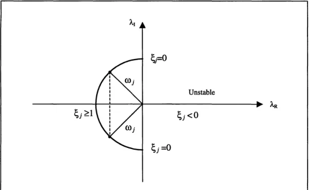
The real term of the right hand side in Equation 2.55 represents an exponentially decay term of the state vector X in Equation 2.44, which is controlled by the modal damping term jwi On the other hand, the imaginary term stands for the oscillation term in X, which is controlled by the damped modal frequency wj, 1-. Figure 2.1 shows this relationship in the complex plane. For the case j < 0, the system is unstable because the response is always amplified by the positive exponential term. When j = 0, the system is undamped because no exponential decay term appears. When 0 < j < 1, the system is underdamped because both exponential decay and oscillation term appear. When j 2 1, the system is overdamped, and only exponential decay term left.

Figure 2.1 Plot of X in complex plane Unstable

Sj<o

(30)

Mode superposition in state-space can be further simplified with the discussion of X. From Equation 2.55, X appears in complex conjugate pair, and each pair share the same

modal damping and modal frequency. Thus, the modes with conjugate pair of eigenvalues have the same properties of dynamic response in the real plane. The only difference they have is the difference in sign of the imaginary oscillation term. The eigenvectors associated with the conjugate pair of eigenvalues have to form conjugate pair in order to produce real state vectors in Equation 2.44 for any time t. Thus, the complex oscillation term cancelled out each other if the effect of the two conjugate responses are combined together. From the above discussion, the dynamic properties of the two conjugate terms are the same, thus the combined effect of response can be treated as a modal response for the system.

Modal analysis is made on the forced vibration response by introducing this concept in Section 2.4.3. From Equation 2.44, the complex conjugate pairs of V and q are identical to the conjugate eigenvalues and eigenvectors mentioned previously. They share the same dynamic properties and can be combined together to represent one modal contribution for the system. Thus, the approximate response can be represented by taking the partial sum of Equation 2.43 as follows

t) = 2[VqiRiR(t)-Vl qi(t)] , l m n (2.56)

i=1

where X is the sum of responses from lower m modes if the eigenvalues and eigenvectors were presorted with the modal frequency to at increasing order. In addition, the same

(31)

procedure can be applied to the analysis of free vibration response by changing the upper limit of the sum of Equation 2.29 to m.

The procedure above is not suitable for all types of analysis. Generally speaking, if the modal frequencies of the modes included in the summation cover the frequency spectrum of the excitation, and the need for response accuracy is not very high, it is acceptable to have only a combination of first several modes. For the example of earthquake, the frequency content is not very high (usually lower than 30 Hz), thus usually five modes are enough to represent the response to an earthquake.

If only the responses of several modes are desired, the computation effort can be further reduced in uncoupling the equations. If first m out of n modes are to be computed, then m right and left eigenvectors are needed to decompose the system. The computation speed is greatly improved by reducing the eigenvalue problem for non-symmetric matrices.

(32)

Chapter 3 Numerical Methods for General Dynamic System

3.1 Numerical Procedure for the Analysis of General Dynamic Systems

The fundamental formulation derived in Chapter 2 is implemented in the numerical algorithms provided in this chapter. The implementation is divided into four major steps. First, the real system parameters are reorganized to form the equivalent state-space formulation. Then the state-space system is transformed into generalized coordinates in complex plane in order to obtain the uncoupled modal system. Then each uncoupled modal system is solved by either direct integration method or frequency domain analysis. The response in each mode is then transform back to real coordinate and sum up to get the total response of the system. The steps are presented below in Figure 3.1.

Form State-space Formulation

Perform Obtain

Modal [ Solution to

De- Each Modal

composition System

Back Trans-formation to Real Coordinate

(33)

Table 3.1 Requirement for Numerical Methods in the Analysis Procedure

Table 3.1 shows the numerical methods required in each step of the procedure. The first step corresponds to the state-space formulations in Section 2.1. As shown in Equation 2.2 to 2.6, the inverse of the mass matrix have to be computed, then several matrix multiplication is needed to form matrix A and the forcing term. After the elements in Equation 2.4 are formed, the system is transformed into uncoupled modal equations in step 2. In order to uncouple the system, procedure for complex eigenproblem in Section 2.2 is performed to obtain the modal system described in Equation 2.15. Thus, complex eigenproblem solver is needed in this step. The solution to each modal equation is obtained after the system is uncoupled into its modal formulation. In this step, either

(34)

direct integration or discrete Fourier transformation is performed to obtain the response of arbitrary excitation. If free vibration problem is considered, step 3 will not be performed. Instead, linear equation solver in step 4 is performed to obtain the solution to the initial value problem. Then, in both of the response cases, i.e., both forced and free response, complex modal effects are combined to produce the real response history of the

system as presented in Section 2.5.

The next sections provide the numerical procedures applied for the analysis. Because the matrix operations and matrix inversion is easier to implement, thus, focus of the following section will be on the complex eigenproblem solver, discrete Fourier transformation and direct integration.

3.2 Numerical Methods for Complex Eigenproblem

The numerical procedure for solving complex eigenproblem is rather difficult compare to its conceptual formulation. Moreover, the eigenvalue of the nonsymmetric matrices are often sensitive to small changes and are even defective. Thus, it is impossible to guarantee an accurate solution to such a problem as is to symmetric eigenproblem [8].

The solution procedure of nonsymmetric eigenproblem is divided into four major steps as shown in Figure 3.2. The first step is balancing, which helps preventing the sensitive problem in the following step. The second step is the reduction procedure to upper

(35)

Hessenberg form. Gaussian elimination with pivoting is introduced to eliminate the lower triangular elements except for the off-diagonal elements. Then, the QR algorithm for real Hessenberg matrices is applied to find the complex conjugate eigenvalues of the matrix. After all the eigenvalues are obtained, several eigenvalues needed proceed with inverse iteration procedure to obtain their corresponding right and left eigenvectors. Descriptions of the procedures are provided in Sections 3.2.1 to 3.2.3.

Part of the

Matrix Reduce to QR Eigen- Inverse

Balancing [- Upper Algorithm values Iteration for

Hessenberg for EZ > Eigenvectors

Form Eigenvalues

Figure 3.2 Procedures for Finding Eigenvalues and Eigenvectors for nonsymmetric matrix

3.2.1 Matrix Balancing and Reduction to Upper Hessenberg Form

Matrix balancing provides a good way to deal with sensitivity with rounding errors and machine accuracy for nonsymmetric matrix. Based on the fact that the errors produced by the system are generally proportional to the Euclidean norm of the matrix, the idea of matrix balancing is to use similarity transformations to obtain a matrix with equal norm in corresponding rows and columns to their pivot elements, thus reduce the norm of the

(36)

matrix. The reason why similarity transformations are applied is to keep the original eigenvalues of the matrix.

The algorithm of balancing comes from Osborne in [8]. It first calculates the row and column norms of the matrix, then calculates the transformation matrix that balances the norm of rows and columns. In order not to worsen the accuracy by the transformations, the elements in the transformation are selected powers of machine radix base.

Notice that if all the eigenvectors are desired, or the inverse iteration is not applied to find the eigenvectors, the similarity transformations have to be kept track of. Because the multiplication of all the similarity transformations made to produce the eigenvalues is the matrix of eigenvectors.

After the balancing procedure is done, the matrix is reduced to upper Hessenberg form. The reason why nonsymmetric matrix can not be directly reduced to diagonal matrix is that the matrix is not symmetrical, the similarity transformation applied on the matrix to cancel out some part of the matrix will not cancel out the symmetric part of it. If one wants to cancel out the other part when one part has become zeros before, then usually the part that has become zero will grow back again because of the transformation. Thus, the upper Hessenberg matrix looks like the following in Figure 3.3 has to be the intermediate state of the solution process. Then different kind of procedure is introduced to search for eigenvalues of the system.

(37)

Non-zero Lower Off-diagonal -Elements Non-zero Upper Triangular Elem Zeros

Figure 3.3 Elements of Upper Hessenberg Matrix

The transformation of the matrix into its upper Hessenberg form can be achieved by any

methods for reducing symmetric matrix to its tridiagonal form. Thus, Givens method, Householder transformation and Gaussian elimination with pivoting are all qualified for the transformation.

The most efficient method among all is Gaussian elimination with pivoting. The reason why Gaussian elimination has to be performed with pivoting is that Gaussian elimination itself is not a similarity transformation. To make the transformation a similarity transformation, column exchanges have to come with corresponding row changes in the transformation of finding pivot element. The procedure of Gaussian elimination with pivoting is as follows:

(38)

1. For stage i of the procedure, the absolute value of the elements below the diagonal elements of the ith column are compared with the diagonal elements, assume the largest element is i+r.

2. Interchange rows i+1 and i+r, also interchange column i+1 and i+r for similarity transformation.

3. For row k greater than i+ 1, subtract ak,i/ai+1,i times row i+ 1 from row k. Also add

ak,i/ai+1,i times column k to column i+ 1 for similarity transformation.

3.2.2 The QR Algorithm for Real Hessenberg Matrix

The QR algorithm of real Hessenberg matrix is adapted from the QR algorithm for tridiagonal matrix. The idea of QR algorithm is based on the fact that any real matrix A can be decomposed by the Householder transformation to the form

A = Q R (3.1)

while keeping its eigenvalues unchanged. The Q matrix in Equation 3.1 is orthogonal and R is upper triangular, assume the next step of Equation 3.1 is

A1 =R-Q=Q'-A-Q

A, = Q1 -R, (3.2)

A2 = R,

Q

= Q'l -A₁Q1

From Equation 3.2, As can be found by repeating the process s times. An important theorem is applied in Equation 3.2 providing a connection of the transform to the solution of eigenvectors. The theorem is stated as follows

(39)

If A has eigenvalues of different absolute value IA.1, then As approaches the upper triangular form as s - o. The eigenvalues appear on the diagonal in decreasing order of

absolute magnitude.

Thus, keep doing the QR decomposition and multiply them in the reverse manner will make the target matrix approaches its eigenvalues. Another useful information in the process of proving the theorem is that the lower-diagonal terms will vanish at the order as follows

a oc( (3.3)

where i>j for lower triangular elements. Equation 3.3 points out a pitfall of the algorithm, that is, if the ith eigenvalue is very close to jth eigenvalue, the convergence may be slow even if the steps s is large. Thus, shifting is introduced to accelerate the convergence rate. Introduce the following equation

A, -k,I =

Q,

R,

(3.4) As+ = R, -Qs +kI = QT -A, -Q,

with all eigenvalues shifted by Ai -ks. The ratio of eigenvalues in Equation 3.3 becomes

a ij oc: 1 -

s

(3.5)

(40)

Another method named implicit shift similar to the shift procedure is developed to prevent the loss of accuracy of small eigenvalues from subtracting operation. The difference between the implicit shift and shift is that the shift is embedded in the transformation matrices instead of directly subtract one of the eigenvalues from the A matrix. The detailed proof of implicit shift can be found from [6] and [8].

The QR algorithm for real Hessenberg matrix is slightly different from the above QR algorithm. This is because complex eigenvalues are expected instead of real eigenvalues. There may exist 2x2 isolated diagonal elements represent complex pairs of eigenvalues. To incorporate this situation, two steps of QR algorithm are combined together using implicit shift to obtain 2x2 diagonals.

Combining two steps of the QR algorithm with shifts in Equation 3.4, Equation 3.6 is obtained

A, sQT = QT -As+₂ (3.6)

Comparing Equation 3.6 to the form of implicit shift as follows

A, .~ . = jT .H (3.7)

From the theorem of implicit shift, if the first column of QT and -' are the same, then matrix Q' and TW are the same and As+2 is equal to H. Thus, the strategy is to find the first row of Q that matches the first row of Q, insert Equation 3.7 into Equation 3.6 to obtain As+2for the next iteration.

(41)

The matrix Q is constructed by a multiplication of series of Householder matrix Pn-, Pn-2

to PI, where P, determines the first row of Q. From the formulation of Householder transformation and the formulation of double shifts, P, is determined as follows

P = _{I- 2wl wT} _(3.8) where (P + _{s,)/+ s,} q, /1 s1 2ww =T r,/s 1

I

[1 ql/(p, s,) r/(p ±s1) 0 .. 0] (3.9) 0 0 and

p, = (ann - a l)(an-.,₁ - aj) - an-1,a,n, + a2a21 q, = a21 [a22 - a, - (an - a11,,) - (a_, - a,,)]

r, = a2 1a32 (3.10)

S= p2 + q2 + r2

Pn-1 to P2 are obtained by the same manner. For example, substitute all, a12, a21 and a32 by

a22, a23, a32 and a43 obtains p2, q2, r2 and s2. Let the normalized pl, q, and r, occupy the

2,3,4 row of the w2 vector, substitute in Equation 3.8 to obtain P2. The detailed derivation

of how to come up with the formulation can also be found from [6] and [8].

The criterion for testing if any eigenvalue has been found is on the test of subdiagonal elements. If the dimension of the matrix is n and if a,,.I is negligible, then a real eigenvalue is found on an,n. Else, if an-2,n-1 is negligible, then there are two real

(42)

eigenvalues or two conjugate complex eigenvalues on the 2x2, anl,n_1 to an,n diagonal

block. Iterate until all the diagonal blocks are found and the corresponding eigenvalues are obtained from the diagonal blocks.

3.2.3 Inverse Iteration for Eigenvectors

After all the eigenvalues are found from QR algorithm for Hessenberg matrix, some selected eigenvalues are thrown into the inverse iteration procedure to obtain their corresponding eigenvectors. In the case of vibration analysis, usually only the response of first five modes are desired. Thus the eigenvalues are first sorted by their absolute value, then first five conjugate pairs of eigenvalues are selected to proceed with inverse

iteration.

The idea of inverse iteration comes from the following equation

(A- - I) -y = b (3.11)

where X is close to one of the eigenvalue X of A, b is a random vector and y is the solution to the equation. The solution y will be close to the eigenvector of k, if X is close enough to it. Thus, the strategy is to iterate for Equation 3.11 by repeatedly replace b by y and solve for the new y. The result of y will be closer and closer to the desired eigenvector.

Notice that if over half of the eigenvectors are desired, recording all the similarity transformation is faster than inverse iteration. Another issue of the inverse iteration

(43)

method is its convergence and accuracy. Because it is an iterative method and the matrix can be defective or has close eigenvectors, good convergence often relies on good initial guess. In addition, because the exact eigenvalues and eigenvectors are not known, when to stop at a reasonable accuracy, or say, making large improvement from the original vector is a big problem. Generally speaking, the strategy is, for large initial growth of lyl, the good guess of initial vector is obtained. If lyl does not grow fast enough, then try another initial vector. After a few iterations, if b does not change much, then the vector is assumed converging, else, recalculate the eigenvalue by Equation 3.12

1 (3.12)

Z

k+1= k +k bky

The criteria presented above ought to be suitable for most of the normal cases. For the defected matrix or closed eigenvectors, some other tricks are provided to deal with the problem. There are discussions about the convergence and accuracy of the method (see [6] and [8]) that provide some answers to those questions.

3.3 Algorithm for Fast Fourier Transformation

As mentioned in Section 2.4.1, Fourier transformation is carried out by integration back and forth from time domain to frequency domain. The response analysis of general dynamic calculates the transfer function as mentioned in Section 2.4.2, multiply it to the corresponding frequency domain excitation to produce a response. The procedure is presented in Equation 2.33 and 2.34.

(44)

Because the input for the system is discrete-time earthquake signals, plus the algorithm for digital computer has to deal with discrete time data, thus the equations have to turn into their discrete form. For Equation 2.31, approximate the integration to finite bounds and rewrite as follows

1 N-I -.2,nm

Fjn fj(tm)e N n = 0, 1, 2..,N -1 (3.13)

n2 m=0

where tm=m At and o=2rtn/NAt. Equation 2.32 can also be rewritten as follows in discrete form

N-i .2;nm

qjm = Hn F e N m =0,1, 2 ...,N -1 (3.14)

n=O

Equation 3.13 together with Equation 3.14 forms a complete discrete Fourier transform pair for mode j.

Looking into the two discrete equations, we can observe that the computation is an O(N2)

process. That means if there are thousands of sampled data, which is normal for seismic analysis, the effort used in carrying the computations is exorbitant. However, by reevaluate the exponential terms in the two equations, the process can be reduced to O(N

log2N).

The reduction proposed by Danielson and Lanczos in 1942 is called Danielson-Lanczos Lemma. The lemma showed that a discrete Fourier transform of length N can be rewritten as the sum of two discrete Fourier transforms each of length N/2. Each subset contains either even numbered data or odd numbered data. The proof of the lemma can be

(45)

accomplished by separating the even and odd numbered points. (Details of the proof and the theory of fast Fourier transformation can be found on [6] and [9].) Furthermore, if N is an integer power of 2, the lemma can be further applied, then the four subsets will have four combination of input data, i.e., even-even, even-odd, odd-even, odd-odd. Continue this process until the data have been subdivided all the way down to transforms of length

1. The transformation of length one is a combination of even and odd data.

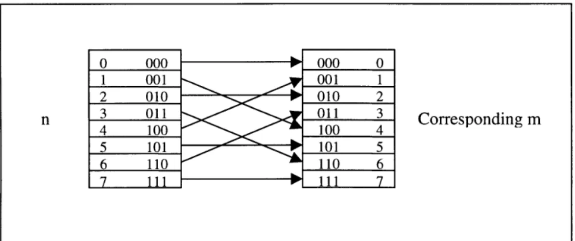
The strategy here is to compute all the possible one-point transform we need. However, the question of this strategy is how to figure out which one-point transformation corresponds to which output. The answer is provided by looking at the pattern of even and odd data combinations in the one-point transformation. For the discrete transformation in Equation 3.13, the way to figure out which m corresponding to which n is to take the bit reversal of the binary value of n. The example of the data ordering for an eight-point Fourier transformation is in Figure 3.4.

o 000 000 0 1 001 001 1 2 010 I 010 2 n 3 011 011 3 Corresponding m 4 100 >100 4 5 101 101 5 6 110 110 6 7 111 P 11 7

(46)

Previous procedure is the basic algorithm of fast Fourier transformation(FFT) proposed by Cooley and Tukey. Notice that this algorithm is for the data length of integer power 2. There are other algorithms dealing with some small power of 2 as a basis of the transformation, for example, 4 (base-4 FFT) and 8 (base-8 FFT). They are also provided in [6] and [9].

There exist problems in the basic FFT algorithm. The first is concerned with the input data. It is very often that the length of the input data set is not equal the integer power of 2. The second is rather a physics problem. If the response of excitation of the system has not died out after the length of FFT, the response near the beginning will be influenced by the end excitation. This is because when the infinite integral is cut into a finite summation form, it is assumed that the excitation is a periodic function. This procedure is valid because our interest is only in a finite period instead of infinite. Thus, although the excitation has been turned into periodic function and the response of it is also periodic, we neglect it and treat it as zero because it is out of the range of our interest. However, problem comes in when there is not enough time for the response of the previous period of excitation to die out and a new one comes in. This is called the wrap-around effect.

There is one simple solution to these problems, which is zero padding. For the first case where the data is not the integer power of 2, padding zeros at the end of input data set to form a complete set with length integer power of 2. For the second case, padding zeros at the end of input data set so that the response dies out before a new period starts. The

(47)

length of padding should be determined by the larger one of the previous two padding cases. Combine the two requirements for zero padding, a criteria comes up as follows

The original length plus the padding length should be the larger length of integer-power-of-two than the length for the response to die out.

To find the padding length meeting this criteria, the length for the response to die out has to be determined first. Equation 3.15 shows the relationship between the decay rate of free response to the number of cycles and the damping ratio.

v _ 2m/'

In = 2 m (3.15)

where n and m are the number of cycles, v is the peak response in the cycle and is the damping ratio. If the desired percentage of decay is 90%, then from equation 3.15, the number of cycle m to die out is as follows

m = In 10 - (3.16)

where the modal damping ratio 4 can be obtained from the modal analysis of the general dynamic system as presented in Section 2.5. The time interval requires to damp out the response is thus mAt, where At is the time step of the discrete system. Thus, if the original time duration is ti, then the total padding time tp needed is as follows

tp = 2 ceil(log 2(t

i

+mAt) ) - ti (3.17)

(48)

The application of FFT in the response of general dynamic system is through Equation 3.13 and 3.14. First, select several modes of interest, throw the data from the eigensystem solver into the FFT algorithm for each mode. Then, multiply the frequency domain transfer functions to each of the corresponding frequency content. Then, do inverse FFT back to the time domain and sum up the response from each mode.

3.4 Algorithm for Direct Integration

Direct integration method is a step-by-step approach that divides the loading and response history into a series of time intervals or "steps". Each of the steps is treated as an independent analysis problem thus only the initial conditions from the previous time step are taken into account. There are generally two kinds of direct integration methods, that is, explicit integration method and implicit integration method. Explicit integration method takes the equilibrium condition at current time step, whereas the implicit integration method takes the equilibrium condition at the next time step. The explicit integration is easier to formulate, and the computation for each time step is less. However, the convergence of the explicit integration method is conditional. Generally speaking, the time interval in the explicit integration method has to be small enough to meet the convergence criteria. For the response history analysis, the time history is usually larger than 15 seconds, and the minimum time interval is limited by the time

(49)

interval of recorded earthquake signal. Thus, the explicit integration method is not suitable for the analysis.

On the other hand, one of the implicit integration method proposed by Newmark provided an unconditionally stable scheme. The method named Newmark method is based on the following assumption on the displacement and velocity in the next time step

t

+At = + [(1 - ) iU+6 "t+t] At _(3.18)

+U=tU+tAt + [(- - a) T + a '+tU] At2 (3.19)

2

where 'U, '0 and 'T are the displacement, velocity and acceleration at time t, and t+AU,

r+A~J and '+At0 are the displacement, velocity and acceleration at time t+At. _c_and₆_are

the control parameters for stability and accuracy. When a = 0.25 and 6 = 0.5, the method becomes unconditionally stable.

In addition to Equation 3.18 and 3.19, the equilibrium equation is taken at time t+At in Equation 3.20

M '+Aj + C ' ~tU + K 'At U = '+AtF (3.20)

Thus three equations, Equation 3.18 to 3.20, are able to solve for three unknowns, the displacement, velocity and acceleration of time t+At. The following procedure is provided as the algorithm of the Newmark method

(50)

1. Initialize 'U, 0U and 0U from the initial conditions. Check if the initial conditions

satisfy the equations of motion at time 0.

2. Select time step At and parameters a and 8. Calculate the following constants:

1 6 1 1

ao = aa 2- a3 = -1;

aAt2 _aAt _aAt _2a

S At 1

a4 -- a= ( )-2; a6=At(1-5); a =SAt;

a 2 2a

3. For given mass matrix M, damping matrix C, and stiffness matrix K, cal

effective stiffness matrix K.

K = aoM + a1C + K 4. Decompose K.

5. For each time step:

a. Calculate the effective load:

t+a =t+AtF + M(ao'U + a2tUJ + a3tU) + C(at U + a4tJ + as'U) b. Solve for the displacement matrix at time t+At

c. Calculate accelerations and velocities at time t+At for the next time step. c. Calculate accelerations and velocities at time t+At for the next time step.

(3.21)

culate the

(3.22)

(3.23)

(3.24)

The procedure can be applied to modal analysis as an alternative method to fast Fourier transformation. For the modal system described in Equation 2.31, the procedure is simplified into a one dimensional problem. After assigning M = 0, C = 1, and K =i, the response is obtained by simply iterating through the procedure.