HAL Id: insu-02413216
https://hal-insu.archives-ouvertes.fr/insu-02413216
Submitted on 20 Dec 2019
HAL is a multi-disciplinary open access
archive for the deposit and dissemination of
sci-entific research documents, whether they are
pub-lished or not. The documents may come from
teaching and research institutions in France or
abroad, or from public or private research centers.
L’archive ouverte pluridisciplinaire HAL, est
destinée au dépôt et à la diffusion de documents
scientifiques de niveau recherche, publiés ou non,
émanant des établissements d’enseignement et de
recherche français ou étrangers, des laboratoires
publics ou privés.
watershed scales
Rebecca Frei, Benjamin W. Abbott, Rémi Dupas, Sen Gu, Gérard Gruau,
Zahra Thomas, Tamara Kolbe, Luc Aquilina, Thierry Labasque, Anniet M.
Laverman, et al.
To cite this version:
Rebecca Frei, Benjamin W. Abbott, Rémi Dupas, Sen Gu, Gérard Gruau, et al.. Predicting nutrient
incontinence in the Anthropocene at watershed scales. Frontiers in Environmental Science, Frontiers,
2020, 7 (200), pp.21. �10.3389/fenvs.2019.00200�. �insu-02413216�
1 2 3 4 5 6 7 8 9 10 11 12 13 14 15 16 17 18 19 20 21 22 23 24 25 26 27 28 29 30 31 32 33 34 35 36 37 38 39 40 41 42 43 44 45 46 47 48 49 50 51 52 53 54 55 56 57 58 59 60 61 62 63 64 65 66 67 68 69 70 71 72 73 74 75 76 77 78 79 80 81 82 83 84 85 86 87 88 89 90 91 92 93 94 95 96 97 98 99 100 101 102 103 104 105 106 107 108 109 110 111 112 113 114 Edited by: Rebecca Elizabeth Tharme, Riverfutures Ltd, United Kingdom Reviewed by: Teresa Ferreira, University of Lisbon, Portugal Luiz Ubiratan Hepp,
Q2
Universidade Regional Integrada do
Q11
Alto Uruguai e das Missões, Brazil *Correspondence: Rebecca J. Frei [email protected]
Specialty section: This article was submitted to Freshwater Science, a section of the journal Frontiers in Environmental Science Received: 22 June 2019 Accepted: 13 December 2019 Published: xx December 2019 Citation: Frei RJ, Abbott BW, Dupas R, Gu S, Gruau G, Thomas Z, Kolbe T, Aquilina L, Labasque T, Laverman A, Fovet O, Moatar F and Pinay G (2019) Predicting Nutrient Incontinence in the Anthropocene at Watershed Scales. Front. Environ. Sci. 7:200. doi: 10.3389/fenvs.2019.00200
Predicting Nutrient Incontinence in
the Anthropocene at Watershed
Scales
Q1 Q3
Rebecca J. Frei1,2*, Benjamin W. Abbott1, Remi Dupas3, Sen Gu4, Gerard Gruau4,
Zahra Thomas3, Tamara Kolbe5, Luc Aquilina4, Thierry Labasque4, Anniet Laverman6,
Ophelie Fovet3, Florentina Moatar7and Gilles Pinay7
1Department of Plant and Wildlife Sciences, Brigham Young University, Provo, UT, United States,2Department of Renewable
Resources, University of Alberta, Edmonton, AB, Canada,3UMR SAS, INRA, AGRO OUEST, Rennes, France,4Univ Rennes,
CNRS, OSUR, Géosciences Rennes, UMR 6118, Rennes, France,5Faculty of Geoscience, Geoengineering and Mining, Q10
Technische Universität Bergakademie Freiberg, Freiberg, Germany,6Centre National de la Recherche Scientifique (CNRS),
ECOBIO – UMR 6553, Université de Rennes, Rennes, France,7RiverLy, Irstea, Lyon, France
Quantifying nutrient attenuation at watershed scales requires long-term water chemistry data, water discharge, and detailed nutrient input chronicles. Consequently, nutrient attenuation estimates are largely limited to long-term research areas or modeling studies, constraining understanding of the ecological characteristics controlling nutrient attenuation and complicating efforts to protect or restore water quality in developed and developing regions. Here, we combined long-term data and a broad suite of biogeochemical parameters from 49 watersheds in northwestern France to test how well instantaneous measurements can predict nitrogen (N) and phosphorus (P) attenuation at watershed scales. We evaluated 13 biogeochemical and 12 hydrological proxies of hydrological flowpaths, residence time, and biogeochemical transformation. Across the 49 watersheds, nutrient attenuation ranged from 88 to −2% for N and 99–96% for P. The strongest biogeochemical proxies of N attenuation were NO−
3 isotopes,
rare earth elements (REEs), radon, and turbidity, together explaining 75% of observed variation. For P attenuation, REEs, NO−
3 isotopes, molecular weight of dissolved organic
matter, and radon were the strongest proxies, but only explained 27% of observed variation. However, a single hydrological parameter—annual runoff—explained 91% of N attenuation and the relative abundance of schist bedrock explained 56% of P attenuation. We discuss how runoff both controls and reflects watershed hydrology, biogeochemistry, and nutrient attenuation. For example, runoff was correlated with long-term decreases in nutrient concentration, demonstrating how leakier watersheds recover more quickly from nutrient saturation. Given the immense fertilization capacity of modern society, we propose that eutrophication can only be solved by reducing nutrient inputs, though hydrochemical proxies can provide valuable information on where to carry out essential food production activities.
115 116 117 118 119 120 121 122 123 124 125 126 127 128 129 130 131 132 133 134 135 136 137 138 139 140 141 142 143 144 145 146 147 148 149 150 151 152 153 154 155 156 157 158 159 160 161 162 163 164 165 166 167 168 169 170 171 172 173 174 175 176 177 178 179 180 181 182 183 184 185 186 187 188 189 190 191 192 193 194 195 196 197 198 199 200 201 202 203 204 205 206 207 208 209 210 211 212 213 214 215 216 217 218 219 220 221 222 223 224 225 226 227 228
INTRODUCTION
Since the Industrial Revolution, humans have more than doubled reactive nitrogen (N) inputs (Gruber and Galloway, 2008) and quadrupled phosphorus (P) inputs (Elser and Bennett, 2011)
Q6
into the Earth’s ecosystems (Seitzinger et al., 2010; Foley et al., 2011; Abbott et al., 2018a). Consequently, 80% of freshwater and coastal ecosystems now experience eutrophication induced by anthropogenic inputs of N and P (Howarth et al., 2000; Galloway Q8
et al., 2003; Poisvert et al., 2017; Le Moal et al., 2019). Though recognized as a planetary priority (Foley et al., 2011; Steffen Q23
et al., 2015; Le Moal et al., 2019), efforts to reduce eutrophication have had mixed results, partly because of two challenges that emerge at watershed scales (i.e., 1–10,000 km2). First, is the difficulty to quantify the overall residence time of nutrients in complex watersheds, which ranges from minutes to millennia as nutrients may be recycled or stored in plant biomass, soil, and groundwater (Jarvie et al., 2013; Sebilo et al., 2013; Marçais et al., 2018; Carey et al., 2019; Kolbe et al., 2019). Second, the capacity of ecosystems to remove or permanently retain nutrients via vertical processes such as denitrification or diagenesis is highly variable, and the socioecological drivers (e.g., watershed characteristics and agricultural practices) of nutrient removal are poorly understood (Pinay et al., 2015; Abbott et al., 2016; Dupas et al., 2018; Goyette et al., 2018; Jarvie et al., 2019).
There are three general fates for nutrients moving through the soils, riparian zones, surface waters, and aquifers of a watershed: (1) Retention (i.e., a long or short-term delay) by biological and physical processes, including nutrient uptake, sorption, or hydrological residence time (Covino et al., 2010; Sebilo et al., 2013; Van Meter et al., 2016; Dupas et al., 2017; Ehrhardt et al., 2019), (2) Vertical removal to the atmosphere or lithosphere, including denitrification, aeolian transport, or mineral precipitation with various metals (Groffman et al., 2006; Seitzinger et al., 2006; Pinay et al., 2018; Randall et al., 2019), and (3) Longitudinal export from the watershed via surface or subsurface flow (Burt and Pinay, 2005; Seitzinger et al., 2010; Abbott et al., 2018a). The reactivity and mobility of organic and inorganic nutrients depend on and influence biogeochemical conditions (Abbott et al., 2016; Bernhardt et al., 2017), meaning that the fate of carbon, N, and P can vary substantially through time (e.g., storm events or seasons) and in space (e.g., different watersheds or biomes) (Dupas et al., 2016; Moatar et al., 2017; Musolff et al., 2017; Minaudo et al., 2019). Consequently, watersheds with similar nutrient inputs often have completely different nutrient export regimes, particularly for headwater watersheds that make up most of the terrestrial-aquatic interface (Bishop et al., 2008; Abbott et al., 2018b; Helton et al., 2018; Wollheim et al., 2018). This variability in nutrient attenuation capacity is likely associated with differences in surface and subsurface characteristics, including differences in water storage capacity and residence times, abundance and activity of biotic nutrient sinks (e.g., plant or microbial assimilation, dissimilatory microbial metabolism) and abiotic factors (e.g., high sorption capacity in soils, mineral precipitation, presence of chemical reducers in bedrock) (Hansen et al., 2002; Aquilina et al., 2012, 2018; Thomas and Abbott, 2018; Kolbe et al., 2019). All these
factors are influenced by changes in hydrological connectivity, uneven distribution of reactants and organisms due to the co-evolution of surface and subsurface characteristics, and the stochastic nature of human and natural disturbance (Hansen et al., 2000; Thomas et al., 2015; Covino, 2017; Moatar et al., 2017).
Despite advances in understanding nutrient dynamics, it remains difficult to quantify nutrient retention and removal on timescales matching hydrological and nutrient residence times (Vitousek, 2004; Pinay et al., 2015; Feng et al., 2018; Ehrhardt et al., 2019). Additionally, many nutrient attenuation studies focus on single-nutrient dynamics, despite the fact that eutrophication is caused by interactions among multiple nutrients and factors (Carpenter et al., 1998; Elser et al., 2007; Paerl et al., 2016; Hobbie et al., 2017; Le Moal et al., 2019). Consequently, there is no straightforward way to predict a watershed’s sensitivity to high nutrient inputs, seriously limiting our ability to prevent eutrophication or improve water quality where it has already been degraded. Quantifying nutrient attenuation at the watershed scale involves lengthy data acquisition and costly infrastructure (Burt, 1994; Howden et al., 2010; Burt et al., 2011), which are not always available in developing nations where agriculture and urbanization are intensifying fastest (Seitzinger et al., 2010; FAO ed., 2017; Dupas et al., 2019b).
In this context of variability, two conceptual approaches for predicting nutrient attenuation are the hot spots/control points concept, which predicts where and when biogeochemical reactions are more likely to occur (McClain et al., 2003; Bernhardt et al., 2017) and the Damköhler number, which uses the ratio of residence time to reaction time to predict how much of a solute can be transformed or retained (Ocampo et al., 2006; Zarnetske et al., 2011; Oldham et al., 2013).Pinay et al. (2015)
and Abbott et al. (2016)proposed to combine these concepts in the HotDam framework by combining multiple proxies of biogeochemical transformation, hydrological flowpaths, and hydrological residence time. Combining or crossing multiple proxies such as solute and isotopic concentrations, hydrograph properties, and organic matter can illustrate terrestrial and aquatic conditions across nutrient flowpaths (Pinay et al., 2015; Abbott et al., 2016; Shogren et al., 2019), potentially paving the way for a more systematic understanding of what controls nutrient attenuation in watersheds. Here, we apply the HotDam framework to identify controls on attenuation of N and P in 49 small to medium watersheds in Brittany, France using a crossed-proxy approach. Our overarching goals were to understand the drivers of nutrient attenuation in agricultural watersheds and test how well nutrient attenuation could be predicted with easily measurable proxies. These proxies included nutrient stoichiometry, organic matter biodegradability, dissolved gases, rare earth elements (REEs), nitrate isotopes, and hydrograph parameters (Figure 1). We hypothesized that nutrient attenuation would be controlled by the hydrological properties of the watersheds (e.g., water residence time and dominant flowpaths), surface and subsurface characteristics (e.g., land use, topography, geology), and biogeochemical conditions (e.g., stoichiometry and spatiotemporal distribution
229 230 231 232 233 234 235 236 237 238 239 240 241 242 243 244 245 246 247 248 249 250 251 252 253 254 255 256 257 258 259 260 261 262 263 264 265 266 267 268 269 270 271 272 273 274 275 276 277 278 279 280 281 282 283 284 285 286 287 288 289 290 291 292 293 294 295 296 297 298 299 300 301 302 303 304 305 306 307 308 309 310 311 312 313 314 315 316 317 318 319 320 321 322 323 324 325 326 327 328 329 330 331 332 333 334 335 336 337 338 339 340 341 342
FIGURE 1 | Conceptual diagram of the crossed-proxy approach we used to investigate controls on watershed-scale nutrient attenuation. We hypothesized that Q4
Q5 watershed-scale nutrient attenuation was a function of water flowpath (red), residence time (purple), and biogeochemical reactivity (pink).
of electron donors and acceptors; see Table 1). We tested these hypotheses by calculating mass balances of N and P for each watershed using 10 years of local, regional, or national agency data, and then sampling the watersheds three times across flow conditions and seasons to analyze the broad suite of proxies.
MATERIALS AND METHODS
Site Description and Experimental Design
The Brittany region of northwestern France has a rich repository of environmental data generated by academic and governmental research. For example, 27 of the 49 watersheds in this study had a nearby surface water monitoring station, which provided the concentration and discharge data necessary to calculate annual nutrient fluxes and long-term trends (Fovet et al., 2015; Thomas et al., 2019) and estimates of nutrient input were available for all watersheds (Poisvert et al., 2017). More generally, these intensively-managed, agricultural landscapes experience high but decreasing nutrient inputs, providing insight into how watershed-level nutrient fluxes respond to changes in nutrient loading (Galloway et al., 2008; Sutton et al., 2013; Poisvert et al., 2017). The region is a part of the Armorican massif which is composed of metamorphic and igneous rock, primarily granite, schist, and micaschist (Aquilina et al., 2012; Goderniaux et al., 2013; Kolbe et al., 2016). The climate is temperate oceanic, with a mean annual temperature of 11.2◦C and mean annual
rainfall ranging from 1,400 mm in the west to 600 mm in the
east, relatively well-distributed throughout the year ( Gascuel-Odoux et al., 2010; Thomas et al., 2015, 2019). The area has an average stream density of about 1 km km−2, relatively shallow
groundwater, and hydromorphic riparian soils that cover about 20% of the land surface (Mourier et al., 2008; Dupas et al., 2013; Marçais et al., 2018). Land use is dominated by row crops, indoor pig and poultry husbandry, and pastureland for cows (a mean of 80% agricultural cover across the study watersheds; Table S1), making Brittany one of the highest density regions in France and Europe for animal breeding (Gascuel-Odoux et al., 2010; Poisvert et al., 2017; Kim et al., 2019). N and P concentrations in many Brittany watersheds are decreasing, attributable primarily to reduction of point sources such as wastewater and feedlot effluent (Moatar et al., 2017; Abbott et al., 2018b; Dupas et al., 2018).
We analyzed stream water chemistry in 49 agricultural watersheds ranging from 2.38 to 2,080 km2(Figure 2). Most of the watersheds were small to medium sized (mean area = 232 km2, median area = 18.2 km2), which was a consequence of
Brittany’s geography as a peninsula and our design to capture variability in headwater watersheds that make up the majority of the land-water interface ((Burt and Pinay, 2005; Bishop et al., 2008; Heathwaite, 2010)). Sampling points were typically near the coast, but above the zone of tidal influence (Figure 2). To capture variable flow conditions and seasonal differences, we collected samples during 3 field campaigns in November 2015 (lowest flow), March 2016 (highest flow), and June 2018 (moderate flow; Figure S1). During each field campaign, we
343 344 345 346 347 348 349 350 351 352 353 354 355 356 357 358 359 360 361 362 363 364 365 366 367 368 369 370 371 372 373 374 375 376 377 378 379 380 381 382 383 384 385 386 387 388 389 390 391 392 393 394 395 396 397 398 399 400 401 402 403 404 405 406 407 408 409 410 411 412 413 414 415 416 417 418 419 420 421 422 423 424 425 426 427 428 429 430 431 432 433 434 435 436 437 438 439 440 441 442 443 444 445 446 447 448 449 450 451 452 453 454 455 456
TABLE 1 | List of proxies in our analysis and predictions of how they might affect nutrient attenuation. Q5
Proxy N attenuation P attenuation Flowpath Residence time Biogeochemical transformation
Explanation
DSi + + + + + + x x Indicator of watershed residence time (Marçais et al., 2018)
δ15N and δ18O + + + − − − x x More enriched NO−
3isotopes indicate
denitrification and requisite conditions (i.e., NO−
3, anoxia, electron donor, denitrifying
bacteria;Lehmann et al., 2003) REE and Ce anomaly + + + − − − x x Ce anomaly is an indirect tracer of redox
conditions and exposure to DOM (Gruau et al., 2004); a larger Ce anomaly correlates with anoxic conditions
Radon + + + + + + x High222Rn indicates deeper flowpaths (Bertin
and Bourg, 1994)
SUVA254 − − − + + + x x SUVA254is an estimate for aromaticity of
organic molecules (Weishaar et al., 2003); higher SUVA254may correlate with lower
bioavailability
SR + + + − − − x x SRis inversely related to molecular weight of
CDOM (Helms et al., 2008); higher SR
correlates with lower molecular weight and may indicate more bioavailable compounds (Ewing et al., 2015)
BDOC + + + − − − x x BDOC measures biodegradability of DOM (McDowell et al., 2006); higher BDOC could stimulate denitrification but also nutrient mineralization
DOC:NO−
3 + + + − − − x x Stoichiometric ratios of C and N can indicate
whether C or N attenuation is more likely (Sterner and Elser, 2002), and also indicate hydrologic flowpath because deep flowpaths have lower C:N ratios
pH + + + − − − x As pH increases, organic colloids become more electronegative and release adsorbed phosphate particles (Gu et al., 2019), and C and N are more available (Glass and Silverstein, 1998)
Turbidity − − − − − − x x Highly turbid systems have large amounts of suspended solids that can export nutrients downstream and limit in-network attenuation Conductivity − − − − − − x x High conductivity can indicate groundwater
inputs or agricultural and urban runoff
Proxies were chosen because they are indicative of hydrologic flowpath, residence time, and/or biogeochemical transformations.
Predicted relationships between proxies and nutrient attenuation assumes increasing concentrations (e.g., higher concentrations of DSi are hypothesized to increase attenuation of N and P).
sampled all 49 sites within 1 week to capture watershed signals in comparable hydrological conditions. Seventeen of the watersheds were independent drainage basins and 32 were nested within the Couesnon and Rance watersheds (23 and 9 nested subwatersheds, respectively), allowing us to assess nutrient attenuation controls across a greater range of watershed sizes (Figure 2) and take advantage of previous research on those sites (Abbott et al., 2018a; Thomas et al., 2019). Though the sub-watersheds of the Couesnon and Rance watersheds are geographically close, they span the Brittany-wide range of observed land use and watershed characteristics (Table S1).
Conceptual Approach
Nutrient retention and removal (hereafter “attenuation”) involve multiple hydrological and biogeochemical processes that are difficult to characterize because many of them are not directly observable due to long timescales or inaccessibility (e.g., groundwater processes) (Aquilina et al., 2018; Kolbe et al., 2019), 3-dimensional variation in soil characteristics (Sebilo et al., 2013; Musolff et al., 2015), and nutrient legacies (Van Meter and Basu, 2017; Ehrhardt et al., 2019). Consequently, to identify the ecological drivers of nutrient attenuation at watershed scales, we selected tracers or proxies that could be associated with hydrological flowpath, residence time, and
457 458 459 460 461 462 463 464 465 466 467 468 469 470 471 472 473 474 475 476 477 478 479 480 481 482 483 484 485 486 487 488 489 490 491 492 493 494 495 496 497 498 499 500 501 502 503 504 505 506 507 508 509 510 511 512 513 514 515 516 517 518 519 520 521 522 523 524 525 526 527 528 529 530 531 532 533 534 535 536 537 538 539 540 541 542 543 544 545 546 547 548 549 550 551 552 553 554 555 556 557 558 559 560 561 562 563 564 565 566 567 568 569 570
FIGURE 2 | (a) Location of the 49 watersheds sampled during the 3 field campaigns (November 2015, March 2016, and June 2018) in Brittany, France. The Couesnon watershed is enlarged to show the 23 nested watersheds in greater detail. (b) Distribution of nutrient concentrations for dissolved organic carbon (DOC), nitrate (NO−
3), and Molybdate-Reactive Phosphorus (MRP). Density plots above the Cartesian planes show seasonal shifts in nutrient concentrations along the x-axis.
biogeochemical reactions (Pinay et al., 2015; Abbott et al., 2016). Informed by the ecological control points concept, which assesses reaction rates in a spatiotemporal context (McClain et al., 2003; Bernhardt et al., 2017); and the Damköhler approach which assesses overall attenuation capacity (Ocampo et al., 2006; Oldham et al., 2013), we attempted to quantify biogeochemical and hydrological controls of N and P attenuation at watershed scales with a crossed-proxy approach (Abbott et al., 2016). We were particularly interested in why relationships between land use and stream nutrient concentrations and fluxes often break down at small scales (Burt and Pinay, 2005; Heathwaite, 2010), and how well watershed characteristics and easily measured proxies could predict nutrient attenuation and shine light on the relative importance of surface and subsurface attenuation
processes (Ben Maamar et al., 2015; Dupas et al., 2019a; Kolbe et al., 2019) and hydrological time lags in soils, sediments, and aquifers (Thomas et al., 2012; Sebilo et al., 2013; Van Meter et al., 2016). To address these questions, we used a diverse set of physicochemical parameters described in detail in the
Supplementary Information (SI: Proxy Toolbox) and briefly outlined below (Figure 1).
Proxies of Hydrological Residence Time
and Flowpath
We used (REEs, dissolved silica (DSi), and Radon-222 as proxies of where water went as it passed through the watershed, what conditions it experienced, and how long it stayed there (SI: Proxy Toolbox). The dissolved REE signature of water is initially
571 572 573 574 575 576 577 578 579 580 581 582 583 584 585 586 587 588 589 590 591 592 593 594 595 596 597 598 599 600 601 602 603 604 605 606 607 608 609 610 611 612 613 614 615 616 617 618 619 620 621 622 623 624 625 626 627 628 629 630 631 632 633 634 635 636 637 638 639 640 641 642 643 644 645 646 647 648 649 650 651 652 653 654 655 656 657 658 659 660 661 662 663 664 665 666 667 668 669 670 671 672 673 674 675 676 677 678 679 680 681 682 683 684 set by the bedrock, but redox conditions can cause selective
changes (Dia et al., 2000; Gruau et al., 2004). Specifically, cerium (Ce) readily oxidizes to Ce+4 and precipitates in the
presence of oxygen (Moffett, 1990; De Carlo et al., 1997; Braun et al., 1998), creating a negative Ce anomaly in water that has experienced consistently oxidizing conditions (Gruau et al., 2004; Pinay et al., 2015). Because redox conditions and organic matter availability strongly influence N and P attenuation processes (e.g., denitrification; P adsorption by Fe-oxyhydroxides) (Stumm and Sulzberger, 1992; Pinay et al., 2015; Gu et al., 2019), we tested the relationship between the Ce anomaly of stream waters with nutrient attenuation at watershed scales. To assess water residence time, we used DSi concentration, which has been found to strongly correlate with subsurface residence time in many hydrogeological contexts (Ayraud et al., 2008; Marçais et al., 2018). Our DSi estimates of residence time, calculated using the empirical relationship derived inMarçais et al. (2018), agreed with estimates derived from chlorofluorocarbons (CFCs) and other dissolved gases from other studies in this region (Molénat et al., 2013; Ben Maamar et al., 2015; Kolbe et al., 2016). Radon-222 (222Rn) is another tool to constrain groundwater-surface water interactions (Bertin and Bourg, 1994; Cable et al., 1996; Stieglitz et al., 2010). A product of natural radioactive decay in igneous bedrock, 222Rn has a half-life of 3.82 days,
making it an ideal tracer of deep flowpaths (Oyarzún et al., 2014). Because deep and long flowpaths increase the likelihood of encountering redox conditions suitable for N removal pathways such as denitrification, we measured222Rn concentration in all
stream water samples.
Proxies of Biogeochemical Transformation
To assess the degree of biogeochemical attenuation of nutrients and the relative importance of nutrient loading vs. nutrient removal, we quantified stable isotopes of NO−
3 (δ15N and
δ18O), optical characteristics and biodegradability of dissolved organic matter (DOM), and nutrient stoichiometry (SI: Proxy Toolbox). Stable isotopes can indicate nutrient source and degree of biogeochemical processing (Mariotti et al., 1981; Lehmann et al., 2003; Malone et al., 2018). NO−
3 isotopes are
particularly useful because NO−
3 is a dominant form of nitrogen
in nutrient saturated ecosystems (Aber et al., 1998), organic and industrial fertilizers have distinct initial δ15N and δ18O (Bedard-Haughn et al., 2003; Lohse et al., 2013; Denk et al., 2017), and denitrification (both heterotrophic and autotrophic) strongly fractionates NO−
3 isotopes, enriching the residual δ15N
and δ18O (Ayraud et al., 2006; Hosono et al., 2014; Malone et al., 2018). Therefore, we predicted that watersheds with isotopically-enriched NO−
3 would have higher N attenuation (Lehmann et al., 2003) or alternatively that they would have primarily organic fertilizer (Bedard-Haughn et al., 2003).
We used multiple characteristics of DOM to assess the degree of biogeochemical processing, nutrient source, and multi-elemental interactions. DOM has been described as a master variable that influences multiple nutrient cycles (e.g., it is a major source of inorganic N and P in nutrient-poor ecosystems) and general physicochemical conditions (McDowell, 2003; Zarnetske et al., 2018). DOM consists of dissolved organic carbon (DOC),
N, P and other nutrients in molecular forms ranging from complex organic molecules to simple compounds. The molecular composition of the DOM influences its biodegradability and photoreactivity, affecting its persistence in the ecosystem and influence on nutrient cycles (Wymore et al., 2018; Harjung et al., 2019). In addition to biodegradability incubations (details below), we calculated two optical proxies of DOM composition: specific ultra-violet absorbance at 254 nm (SUVA254) and the
spectral ratio (SR) of slopes within the 275–290 and 350–400 nm
range (Weishaar et al., 2003; Helms et al., 2008; Vonk et al., 2015). DOM concentration and characteristics can also indicate hydrological flowpaths because DOM is less abundant and more microbially altered in groundwater (Shen et al., 2015; Mu et al., 2017; Coble et al., 2019).
Nutrient stoichiometry, which is based on conservation of mass and constant proportions in many organisms, allows prediction of retention or release of different compounds based on availability and relative demand (Sterner and Elser, 2002; Allen and Gillooly, 2009; Helton et al., 2015). We used nutrient ratios as metrics of flowpath and biogeochemical transformation. For example, a negative relationship between DOC and NO− 3
has been widely observed in freshwater and estuarine ecosystems (Sterner and Elser, 2002; Taylor and Townsend, 2010; Stubbins, 2016). This relationship has been primarily attributed to stoichiometric controls, where abundant DOC promotes NO− 3
removal via denitrification since DOC is the most common electron donor and in high-DOC watersheds oxygen could be depleted more rapidly due to mineralization of DOC, resulting in more anoxic zones where denitrification can occur (Arango et al., 2007; Fork and Heffernan, 2013; Helton et al., 2015). Alternatively, the negative relationship between DOC and NO− 3
could simply be caused by a negative correlation between sources, where watersheds that favor deeper hydrological flowpaths have a carbon-poor and nitrogen-rich signal (Abbott et al., 2018b). Therefore, we predicted higher nutrient attenuation in catchments with greater DOC:NO−
3 ratios.
Hydrograph Metrics
The characteristics of river flow can indicate fundamental hydrological properties at watershed scales (Fang and Shen, 2017; Moatar et al., 2017). Higher peak flows during storm events can indicate greater near-surface runoff, while less responsive hydrographs and higher base flows between events can indicate longer residence time and greater proportion of subsurface flow (Feijoó et al., 2018; Kirchner, 2019). In this context, we calculated several, non-redundant hydrological metrics (see Table S2) based on daily stream flow: (i) the mean, (ii) coefficient of variation, (iii) skewness, (iv) kurtosis, (v) the autoregressive lag-one correlation coefficient (AR1), (vi) the amplitude, (vii) the phase of the seasonal signal (Archfield et al., 2014), and (viii) the W2. The W2 is an index of hydrologic reactivity that is the percentage of annual discharge that occurs during the highest 2% of flows (Walsh and Lawler, 1981; Moatar et al., 2013, 2017).
Field and Laboratory Analysis
To quantify the proxies described above, we collected water samples and measurements from 49 watersheds throughout
685 686 687 688 689 690 691 692 693 694 695 696 697 698 699 700 701 702 703 704 705 706 707 708 709 710 711 712 713 714 715 716 717 718 719 720 721 722 723 724 725 726 727 728 729 730 731 732 733 734 735 736 737 738 739 740 741 742 743 744 745 746 747 748 749 750 751 752 753 754 755 756 757 758 759 760 761 762 763 764 765 766 767 768 769 770 771 772 773 774 775 776 777 778 779 780 781 782 783 784 785 786 787 788 789 790 791 792 793 794 795 796 797 798 Brittany, France (Figure 2). We selected the 49 sites based on
accessibility, availability of historical data (nutrient input and export chronicles and land-use data), and to cover a range of watershed sizes. Field campaigns were in early November of 2015, late March of 2016, and late June of 2018.
At each site, we collected one 5-L sample of stream water for immediate sensor readings and eight smaller samples for laboratory analyses. From the first sample, we used a handheld multiparameter probe (YSI, incorporated; Yellow Springs, USA) to measure dissolved oxygen, redox, pH, temperature, and turbidity. We determined SUVA254and SRfrom the same sample
with a field-deployable spectrophotometer (s::can; Vienna, Austria). For the lab analyses, we immediately filtered subsamples using a 50 mL syringe and two 250 mL filter towers. We used a 0.2 µm cellulose acetate syringe filter to prepare samples for the analysis of cations, REEs, and NO−
3 isotopes. For the first
filter tower, we used a 0.45 µm cellulose acetate filter to prepare samples for Molybdate-Reactive Phosphorus (MRP), anions, and DOC analysis. For the second tower, we used a 0.7 µm glass fiber filter, which removes most particulates but allows many bacteria to pass (Vonk et al., 2015), to prepare samples for the biodegradable DOC (BDOC) bioassay experiment. All filters, towers, and syringes were pre-rinsed with de-ionized water and flushed with sample prior to collecting final samples. We also collected an unfiltered, bubble-free 200 mL sample for 222Rn analysis. These samples were analyzed for 222Rn within 12 h of sampling using a radon detector (Durridge RAD7 analyzer, Billerica, USA), with most samples analyzed immediately in the field. Delayed samples were adjusted for time lags to correct222Rn
decay. The222Rn values for the spring sampling were lost due to
operator error.
MRP concentrations were determined colorimetrically via reaction with ammonium molybdate (Murphy and Riley, 1962),
Q12
with a precision of ±4 µg l−1 (Gu et al., 2018). Nitrate
isotope samples were frozen immediately and shipped to the UC Davis Stable Isotope Facility for analysis of δ15N
and δ18O of NO−
3 by bacterial denitrification assay (McIlvin and Casciotti, 2011). Isotope ratios of δ15N and δ18O were
measured using a ThermoFinnigan GasBench + PreCon trace gas concentration system connected to a ThermoScientific Delta V Plus isotope-ratio mass spectrometer (Bremen, Germany) with a precision of ± 0.4‰ and 0.5‰ for δ15N and δ18O, respectively.
Cations and REE samples were analyzed by inductively coupled plasma mass spectrometry (ICP-MS; Agilent 7700×, Santa Clara, USA). Calibration curves and accuracy controls were performed following best practices (Yeghicheyan et al., 2013), using river water reference material for trace elements with a wide compositional range (SLRS-5, National Research Council of Canada). De-ionized water purified with a Milli-Q (Millipore, Darmstadt, Germany) system was used for blanks. Total relative uncertainties were ±5%.
We conduced BDOC bioassay experiments using four replicates of 100 mL aliquots of filtered stream water for each site and incubated in a dark incubation chamber for 28 days at 20◦C (Vonk et al., 2015). We sampled each replicate at the
beginning (t0) and end of the incubation (t28). The t0 samples
were acidified with 6M HCl to a pH of 2 and stored in the refrigerator at 4◦C until the t
28 sampling. After the t28samples
were acidified, the t28 and t0 samples were analyzed together
for DOC (Shimadzu TOC-5050A, Kyoto, Japan, precision ±5%) within 1 week. We calculated the percent BDOC for each sample using the following equation:
%BDOC = DOCt0−DOCt28 DOCt0
∗100% (1)
where DOCt0and DOCt28 are the concentrations of DOC at t0
and t28. We reported the mean of the 4 replicates as the overall
BDOC value per sampling for each site.
Watershed Characteristics and Nutrient
Trends
To test how climate and landscape characteristics affect nutrient attenuation, we delineated all watersheds using ArcMap (ESRI) and extracted landscape characteristics including vegetation cover, land use, bedrock type, river network density, and flow regulation. Mean annual temperature and precipitation were downloaded from the WorldClim database (Fick and Hijmans, 2017) using the “raster” package in R (Version 3.5.2; R Core Team, 2018). To obtain long-term nutrient and hydrological discharge data, we selected monitoring stations using the “Near” tool in ArcMap. We obtained long-term data for 27 of the 49 watersheds and calculated annual runoff, nutrient flux, and attenuation for those 27 watersheds using 10 years of flow and water chemistry data (NO−
3 and TP) from July 2008–July 2018.
We calculated the eight flow metrics described above from the flow time series using the EflowStats R package.
We calculated mean annual specific discharge by averaging the flow per year and dividing by watershed area. We calculated N and P fluxes exported from the watershed using the discharge-weighted concentration method (Moatar et al., 2013; Raymond et al., 2013): Flux = k ∗ Q ∗ P iPCi ∗ Qi iQi (2) where Ci and Qi represent concentration and runoff at the time of sampling, Q is mean annual runoff, and k is a conversion factor to obtain fluxes in kg N or P ha−1 yr−1. We calculated
apparent attenuation of NO−
3 and TP using the following
mass-balance equation:
Attenuation = 1 − Flux
Surplus (3)
where Flux is calculated as described above (Equation 2) and Surplus is the watershed-specific nutrient surplus based on fertilizer inputs and crop yields (Poisvert et al., 2017; Dupas et al., 2018).
Because not all watersheds had nearby water quality and discharge stations, we calculated another metric of nutrient attenuation: the residuals from a regression of NO−
3 or TP
799 800 801 802 803 804 805 806 807 808 809 810 811 812 813 814 815 816 817 818 819 820 821 822 823 824 825 826 827 828 829 830 831 832 833 834 835 836 837 838 839 840 841 842 843 844 845 846 847 848 849 850 851 852 853 854 855 856 857 858 859 860 861 862 863 864 865 866 867 868 869 870 871 872 873 874 875 876 877 878 879 880 881 882 883 884 885 886 887 888 889 890 891 892 893 894 895 896 897 898 899 900 901 902 903 904 905 906 907 908 909 910 911 912 metric is much coarser than the mass-balance estimates of
attenuation (Equation 3), it provided an independent metric of attenuation that was quantifiable even for watersheds without discharge and long-term data. Additionally, it allowed calculation of seasonal dynamics in the relationship between land use and nutrient concentration, whereas the mass-balance-based nutrient attenuation metric provided a single value derived from the entire decadal time series. We reasoned that because most nutrient inputs in this region come from agricultural activity, watersheds with nutrient concentrations above the trend line would be less attenuative and points below the line would be more attenuative, comparatively to the average data set (Figure 3). We used NO− 3
concentration for these calculations because it accounted for 92% of measured total N, and TP to account for all measured P (Figure S2).
One weakness of both the mass-balance and residual metrics of nutrient attenuation is that apparent attenuation can occur if significant time lags exits between nutrient inputs and export (Basu et al., 2011; Ehrhardt et al., 2019). Over the past two decades, agricultural practices have improved and many nutrient point sources have been eliminated in western France (Poisvert et al., 2017; Abbott et al., 2018b; Dupas et al., 2018), and we reasoned that the slope of the decline in nutrient concentration would be negatively correlated with hydrological nutrient legacy (i.e., watersheds with more groundwater and soil nutrient storage would have slower rates of nutrient decrease after inputs ceased or were reduced). For the 27 watersheds with long-term data, we calculated Theil-Sen slope estimates using the Siegel method, which provides an estimate of change through time that is highly robust to extreme values due to real variability (e.g., during high or low flows) or analytical errors (Abbott et al., 2018b). We correlated these slope estimates with the nutrient attenuation metrics to assess how much of the apparent attenuation could be due to hydrological
nutrient legacy rather than more permanent removal and retention processes.
Quantifying Spatial Stability and Identifying
Drivers of Nutrient Attenuation
We determined the persistence of spatial patterns through time for proxies and water chemistry across watersheds using the spatial stability concept (Abbott et al., 2018a; Dupas et al., 2019b). The Spearman rank correlation between each pair of sampling dates for each parameter indicates how much of the spatial structure is preserved through time. Spatial stability of water chemistry can result from high spatial variability and synchronous temporal variability (Abbott et al., 2018a; Dupas et al., 2019b).
To disentangle the controls on nutrient attenuation, we regressed each proxy against nutrient attenuation (mass balance and residuals) and fluxes. We used pairwise correlation and multiple linear regression (MLR) to identify which proxies were the most closely associated with nutrient attenuation. Because many of the proxy data were not linearly related with attenuation and fluxes, we used Spearman correlations to quantify the strength of relationships. For the MLR models we grouped predictors into two categories: biogeochemical proxies and hydrological and watershed characteristics (hereafter referred to as the proxy and hydro models, respectively). To test our hypotheses about controls on nutrient attenuation, we categorized each predictor based on whether it was most associated with hydrological and watershed characteristics or biogeochemical reactions (Figure 1, Table 1). We standardized all predictors (mean = 0 and standard deviation = 1) to allow comparison of parameter coefficients as a measure of relative contribution to model prediction of the response variable (nutrient mass balance estimates), and we checked for multicollinearity among predictors using the variance
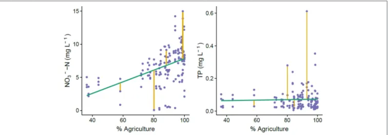
FIGURE 3 | Visualization of how we calculated residuals in the relationship between agricultural land use and nutrient concentrations for each catchment. Because agriculture is the predominant nutrient source in the Brittany region, we used departure from the relationship between agriculture and nutrient concentration as a metric of nutrient attenuation capacity. Points above the regression line represent less attenuation capacity because there is more nutrient in the system than would be expected with this rough estimate of nutrient inputs.
913 914 915 916 917 918 919 920 921 922 923 924 925 926 927 928 929 930 931 932 933 934 935 936 937 938 939 940 941 942 943 944 945 946 947 948 949 950 951 952 953 954 955 956 957 958 959 960 961 962 963 964 965 966 967 968 969 970 971 972 973 974 975 976 977 978 979 980 981 982 983 984 985 986 987 988 989 990 991 992 993 994 995 996 997 998 999 1000 1001 1002 1003 1004 1005 1006 1007 1008 1009 1010 1011 1012 1013 1014 1015 1016 1017 1018 1019 1020 1021 1022 1023 1024 1025 1026 inflation factor (Abbott and Jones, 2015). We ran the models
for each category (i.e., proxy and hydro models) and selected the most parsimonious model for each by stepwise regression. Though model selection techniques continue to be controversial in ecology (reviewed in Malone et al., 2018), our primary goal was to assess relative influence of the major predictors. As such, we simply discuss the overall trends (e.g., what parameters appeared repeatedly in multiple models) of individual and multiple regression results (Tables 2, 3) and we abstain from interpreting the inclusion or exclusion of less influential predictors.
RESULTS
Nutrient Context and Spatial Stability of
Water Chemistry
The three samplings captured distinct hydrological conditions, with low but variable discharge among sites in the fall sampling (November of 2015), highest discharge in the spring (March of 2016), and low and consistent discharge among sites in the summer (June of 2018; Figure S1). Nutrient concentrations and stoichiometry varied substantially across the watersheds and through time (e.g., 0–15 mg L−1 of N-NO−
3 and 0–
0.6 mg L−1 of MRP). We observed a negative relationship
between DOC and NO−
3 and a positive relationship between
DOC and MRP, which varied somewhat seasonally (Figure 2b,
Figure S1). Inorganic forms of N and P dominated total concentrations for these nutrients across watersheds, with NO− 3
making up 93% of total N and MRP making up 74% of TP (Figure S2).
For the 27 watersheds with decadal nutrient concentration data on a monthly time step, the long-term trends were fundamentally different for C, N, and P (Figure 4). Theil-Sen slope estimates for DOC concentration indicated slight increases through time for 75% of the watersheds, decreases for NO− 3
concentration for all but three watersheds, and no change for PO3−4 and TP concentrations (Figure 4).
Spatial stability (persistence of spatial rankings through time) varied substantially among proxies and solutes (Figure 5). Conductivity, δ15N, TP, DSi, and many major ions showed high spatial stability (i.e., more than half the spatial pattern among the three sampling dates was preserved; ρ > 0.7). All the DOM properties,222Rn, O
2, temperature, and NO−2 showed very
low stability (i.e., ρ < 0.4) indicating substantial seasonal and potentially interannual variability, with the rest of the parameters showing moderate stability (Figure 5).
Differences in Attenuation and Fluxes in
Agricultural Watersheds
Median nutrient attenuation as calculated by mass balance was 58.1% for N and 98.6% for P across the watersheds. N and P mass balance results were weakly correlated (R2
= 0.18, p < 0.001), indicating that watersheds with high attenuation for N tended to also have high attenuation for P (Figure 6). Results for N mass balance showed substantially higher variability than P mass balance, ranging from −2 to 88.4% for N but only 96.1 to 99.5% for P. As another estimate of nutrient attenuation, we calculated the residuals of the regression of percent agricultural cover and measured NO− 3
and TP concentrations (Figure 3). N-NO−
3 was significantly
correlated with agricultural cover (R2 = 0.21, p < 0.001) and residuals from that relationship ranged from −7.23 to 6.93 mg L−1 with a median of −0.37 mg L−1. TP was not significantly
correlated with agricultural cover (R2 = 0.001, p = 0.70) and
residuals from that non-significant relationship ranged from −0.54 to 0.047 mg L−1 with a median of 0.016 mg L−1. N
residuals showed a weak, positive correlation with N mass balance estimates (R2 = 0.15, p < 0.001; Figure 6), but we
observed no relationship between P residuals and P mass balance (Figure 6).
N fluxes varied by an order of magnitude (6.1–64 kg N ha−1
yr−1) and were negatively correlated with mass balance estimates
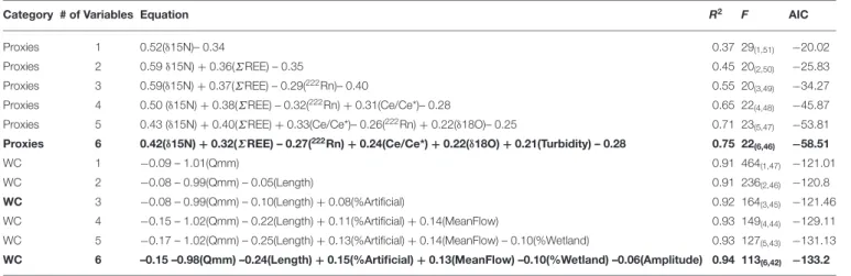
TABLE 2 | Multiple linear regression models for N attenuation using proxies and watershed characteristics (WC). Q22
Q22
Category # of Variables Equation R2 F AIC
Proxies 1 0.52(δ15N)– 0.34 0.37 29(1,51) −20.02
Proxies 2 0.59 δ15N) + 0.36(ΣREE) – 0.35 0.45 20(2,50) −25.83
Proxies 3 0.59(δ15N) + 0.37(ΣREE) – 0.29(222Rn)– 0.40 0.55 20
(3,49) −34.27
Proxies 4 0.50 (δ15N) + 0.38(ΣREE) – 0.32(222Rn) + 0.31(Ce/Ce*)– 0.28 0.65 22
(4,48) −45.87
Proxies 5 0.43 (δ15N) + 0.40(ΣREE) + 0.33(Ce/Ce*)– 0.26(222Rn) + 0.22(δ18O)– 0.25 0.71 23
(5,47) −53.81
Proxies 6 0.42(δ15N) + 0.32(ΣREE) – 0.27(222Rn) + 0.24(Ce/Ce*) + 0.22(δ18O) + 0.21(Turbidity) – 0.28 0.75 22
(6,46) −58.51
WC 1 −0.09 – 1.01(Qmm) 0.91 464(1,47) −121.01
WC 2 −0.08 – 0.99(Qmm) – 0.05(Length) 0.91 236(2,46) −120.8
WC 3 −0.08 – 0.99(Qmm) – 0.10(Length) + 0.08(%Artificial) 0.92 164(3,45) −121.46
WC 4 −0.15 – 1.02(Qmm) – 0.22(Length) + 0.11(%Artificial) + 0.14(MeanFlow) 0.93 149(4,44) −129.11
WC 5 −0.17 – 1.02(Qmm) – 0.25(Length) + 0.13(%Artificial) + 0.14(MeanFlow) – 0.10(%Wetland) 0.93 127(5,43) −131.13
WC 6 –0.15 –0.98(Qmm) –0.24(Length) + 0.15(%Artificial) + 0.13(MeanFlow) –0.10(%Wetland) –0.06(Amplitude) 0.94 113(6,42) −133.2
1027 1028 1029 1030 1031 1032 1033 1034 1035 1036 1037 1038 1039 1040 1041 1042 1043 1044 1045 1046 1047 1048 1049 1050 1051 1052 1053 1054 1055 1056 1057 1058 1059 1060 1061 1062 1063 1064 1065 1066 1067 1068 1069 1070 1071 1072 1073 1074 1075 1076 1077 1078 1079 1080 1081 1082 1083 1084 1085 1086 1087 1088 1089 1090 1091 1092 1093 1094 1095 1096 1097 1098 1099 1100 1101 1102 1103 1104 1105 1106 1107 1108 1109 1110 1111 1112 1113 1114 1115 1116 1117 1118 1119 1120 1121 1122 1123 1124 1125 1126 1127 1128 1129 1130 1131 1132 1133 1134 1135 1136 1137 1138 1139 1140
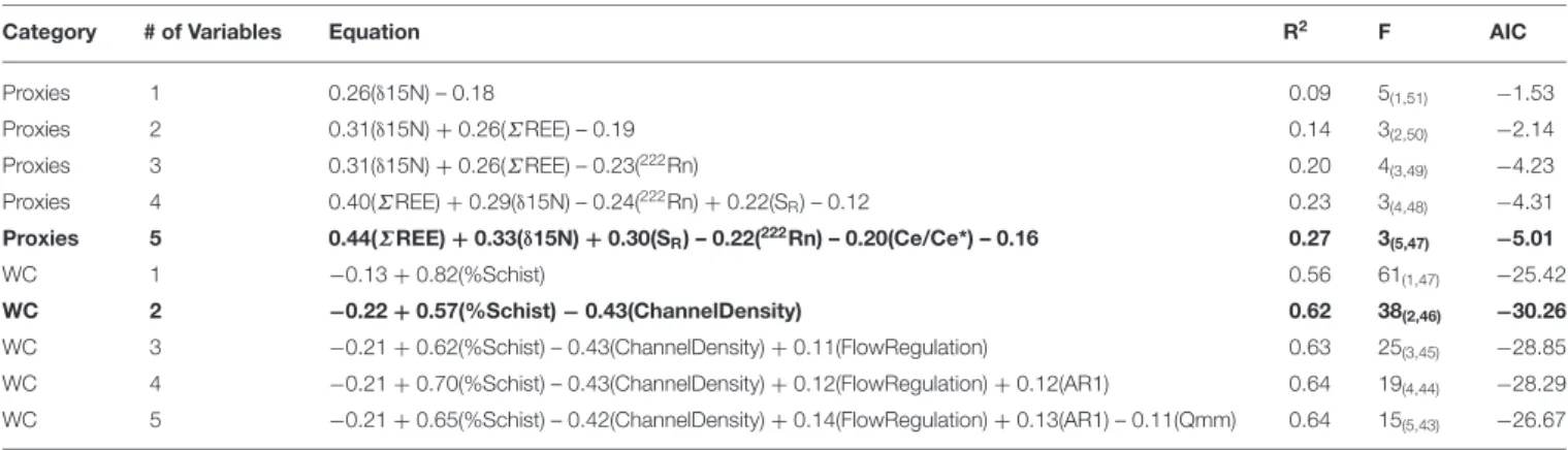
TABLE 3 | Multiple linear regression models for P attenuation using proxies and watershed characteristics (WC). Q22
Category # of Variables Equation R2 F AIC
Proxies 1 0.26(δ15N) – 0.18 0.09 5(1,51) −1.53 Proxies 2 0.31(δ15N) + 0.26(ΣREE) – 0.19 0.14 3(2,50) −2.14 Proxies 3 0.31(δ15N) + 0.26(ΣREE) – 0.23(222Rn) 0.20 4 (3,49) −4.23 Proxies 4 0.40(ΣREE) + 0.29(δ15N) – 0.24(222Rn) + 0.22(S R) – 0.12 0.23 3(4,48) −4.31
Proxies 5 0.44(ΣREE) + 0.33(δ15N) + 0.30(SR) – 0.22(222Rn) – 0.20(Ce/Ce*) – 0.16 0.27 3(5,47) −5.01
WC 1 −0.13 + 0.82(%Schist) 0.56 61(1,47) −25.42
WC 2 −0.22 + 0.57(%Schist) − 0.43(ChannelDensity) 0.62 38(2,46) −30.26
WC 3 −0.21 + 0.62(%Schist) – 0.43(ChannelDensity) + 0.11(FlowRegulation) 0.63 25(3,45) −28.85
WC 4 −0.21 + 0.70(%Schist) – 0.43(ChannelDensity) + 0.12(FlowRegulation) + 0.12(AR1) 0.64 19(4,44) −28.29
WC 5 −0.21 + 0.65(%Schist) – 0.42(ChannelDensity) + 0.14(FlowRegulation) + 0.13(AR1) – 0.11(Qmm) 0.64 15(5,43) −26.67
We considered models with 1–6 predictors and bolded the most parsimonious model in each category based on AIC. All predictors were standardized (mean = 0 and standard deviation =1) to allow comparison of parameter coefficients as a measure of relative contribution to model prediction of the response variable (greater absolute value means more influential). Full models contained all variables within a category (e.g., measured proxies or watershed characteristics calculated or extracted from GIS) and the most parsimonious model (emphasized in bold) was chosen using the Akaike information criterion (AIC).
FIGURE 4 | The distribution of Theil-Sen nutrient slopes for C, N, and P for the 27 watersheds with long-term nutrient data. Horizontal gray lines indicate zero slope (no temporal trend).
(R2 =0.73, p < 0.001), with fluxes increasing as mass balance estimates decreased (Figure 6). P fluxes varied by a factor of 4 (0.17–0.69 kg P ha−1yr−1) and were negatively correlated with P
mass balance (R2=0.36, p < 0.001), but there was no relationship
with P residuals.
Individual Predictors of Nutrient
Attenuation
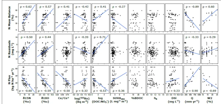
Based on the pairwise Spearman correlations with hydrological parameters, annual runoff was strongly negatively correlated with the N and P mass balance estimates (ρ = −0.89 and −0.41, respectively), and the hydrological reactivity index (W2) was
strongly positively correlated with N and P mass balance (ρ =0.60 and 0.32, respectively). For biogeochemical proxies, N mass balance estimates was correlated with δ15N and δ18O, 222Rn, Ce/Ce∗, and DOC:NO−
3 stoichiometry (ρ > |0.40|) and
had a weaker relationship with SUVA254(ρ = −0.27; Figure 7).
N residuals showed similar results for δ15N and δ18O (ρ > 0.40) but had a much weaker relationship with222Rn, a much stronger relationship with DOC:NO−
3 (ρ = −0.20 and 0.71,
respectively), and no significant relationship with Ce/Ce∗ or
SUVA254. N fluxes showed similar but opposite relationships as
attenuation, and a weak relationship with DSi was also observed (ρ = 0.23). P mass balance estimates was positively correlated
1141 1142 1143 1144 1145 1146 1147 1148 1149 1150 1151 1152 1153 1154 1155 1156 1157 1158 1159 1160 1161 1162 1163 1164 1165 1166 1167 1168 1169 1170 1171 1172 1173 1174 1175 1176 1177 1178 1179 1180 1181 1182 1183 1184 1185 1186 1187 1188 1189 1190 1191 1192 1193 1194 1195 1196 1197 1198 1199 1200 1201 1202 1203 1204 1205 1206 1207 1208 1209 1210 1211 1212 1213 1214 1215 1216 1217 1218 1219 1220 1221 1222 1223 1224 1225 1226 1227 1228 1229 1230 1231 1232 1233 1234 1235 1236 1237 1238 1239 1240 1241 1242 1243 1244 1245 1246 1247 1248 1249 1250 1251 1252 1253 1254
FIGURE 5 | Spatial stability of biogeochemical tracers and chemical concentrations across all 49 watersheds. Parameters are grouped thematically by color. Solutes with a Spearman’s ρ above the horizontal line maintain more than half the spatial pattern for that parameter in pairwise comparisons among the three sampling dates.
with δ15N and δ18O (ρ = 0.41 and 0.29, respectively; Figure 8)
and negatively correlated with 222Rn (ρ = −0.35). P residuals were strongly negatively correlated with δ15N and222Rn (ρ = −0.52 and −0.44, respectively) and had weaker relationships with δ18O, Ce/Ce∗, and S
R(ρ < |0.25|). The P fluxes had similar
but opposite relationships with the same proxies as attenuation, in addition to a negative relationship with DOC:NO− 3
(ρ = −0.40).
To test how nutrient legacy could be related to apparent nutrient attenuation, we correlated the decadal Theil-Sen concentration slopes (Figure 4, Figure S3) with estimates of nutrient attenuation. N mass balance estimates and residuals were positively correlated with decadal trends for NO−
3,
indicating that the watersheds experiencing the slowest decreases in NO−
3 through time tended to have higher apparent attenuation
(R2=0.17 and 0.10, respectively, p < 0.05; Figure S3). N flux was negatively correlated with decadal NO−
3 trends, indicating
that watersheds with faster decreases in NO−
3 had higher N fluxes
(R2=0.25, p < 0.05). PO3–
4 slopes were positively correlated with
P mass balance estimates (R2 =0.15, p < 0.05), indicating that the watersheds with the slowest decreases or greatest increases in PO3–4 had higher apparent P attenuation, but PO3–4 slopes were not significantly correlated with P residuals. TP fluxes were negatively correlated with NO−
3 trends (R2=0.27, p < 0.05).
Multiple Linear Regression Models of
Nutrient Attenuation
For the hydro MLR models (only hydrological and watershed characteristics parameters), the models with only one predictor explained 91% of the variance explained by annual runoff for N mass balance estimates and 62% of the variance explained by the abundance of schist bedrock for P mass balance (see Tables 2,
3). The most parsimonious (based on AIC) hydro model for N mass balance estimates also included other hydrological and land use variables (e.g., mean annual flow and amplitude, and % artificial land cover, wetlands, and stream length), which slightly enhanced the model performance (adjusted R2 = 0.94, 1AIC = 12.19). For P mass balance estimates, the initial hydro model (i.e., only relative abundance of schist) was improved by adding river density (adjusted R2 = 0.62,
1AIC = 4.84). The final hydro model results are shown in Figure 9.
The proxy MLR models that used biogeochemical proxies to predict attenuation did not explain as much variance as the hydro models, but they indicated other processes besides runoff and bedrock type that are important drivers of attenuation. For example, the single most important proxy for N was δ15N, which accounted for 37% of the variation in N mass balance estimates. However, the most parsimonious model
1255 1256 1257 1258 1259 1260 1261 1262 1263 1264 1265 1266 1267 1268 1269 1270 1271 1272 1273 1274 1275 1276 1277 1278 1279 1280 1281 1282 1283 1284 1285 1286 1287 1288 1289 1290 1291 1292 1293 1294 1295 1296 1297 1298 1299 1300 1301 1302 1303 1304 1305 1306 1307 1308 1309 1310 1311 1312 1313 1314 1315 1316 1317 1318 1319 1320 1321 1322 1323 1324 1325 1326 1327 1328 1329 1330 1331 1332 1333 1334 1335 1336 1337 1338 1339 1340 1341 1342 1343 1344 1345 1346 1347 1348 1349 1350 1351 1352 1353 1354 1355 1356 1357 1358 1359 1360 1361 1362 1363 1364 1365 1366 1367 1368
FIGURE 6 | Relationships among our metrics of nutrient attenuation. Here, “Mass Balance” refers to the mass balance estimates of attenuation, “Flux” refers to the fluxes of those nutrients from the watersheds based on concentration and discharge data, and “Residuals” refers to the remaining variation in nutrient concentration after accounting for differences in agricultural land cover (Figure 3). Trend lines for significant correlations (p < 0.05) are shown and R2-values are reported.
included 5 other proxies (ΣREE, 222Rn, Ce/Ce∗, δ18O, and
turbidity), together accounting for 75% of the variation in N mass balance estimates. For P mass balance estimates, the single most important proxy was also δ15N, accounting for
9% of the variation. However, the most parsimonious model included 4 other proxies (ΣREE, SR, 222Rn, and Ce/Ce∗),
together explaining 27% of the variation in P mass balance estimates. Furthermore, the shared proxies between N and P attenuation models (e.g., δ15N, ΣREE, 222Rn, and Ce/Ce∗)
had surprisingly similar relationships in both direction and magnitude, apart from Ce/Ce∗which had a positive relationship
with N mass balance estimates and a negative relationship with P mass balance estimates. Proxy model results are shown in Figure 9.
DISCUSSION
We hypothesized that hydrological properties, surface and subsurface characteristics, and biogeochemical conditions would interact to determine nutrient attenuation at watershed scales. Based on our analysis of 49 watersheds, 27 of which had long-term nutrient and discharge estimates, hydrological properties set the initial attenuation capacity, with secondary effects from biogeochemical conditions and land-use parameters. These results corroborate findings from other regions where runoff strongly controls nutrient attenuation and flux (Covino et al., 2010; Zarnetske et al., 2018; Ehrhardt et al., 2019). However, we point out that runoff is a high-level parameter that interacts with other hydrological metrics, watershed
1369 1370 1371 1372 1373 1374 1375 1376 1377 1378 1379 1380 1381 1382 1383 1384 1385 1386 1387 1388 1389 1390 1391 1392 1393 1394 1395 1396 1397 1398 1399 1400 1401 1402 1403 1404 1405 1406 1407 1408 1409 1410 1411 1412 1413 1414 1415 1416 1417 1418 1419 1420 1421 1422 1423 1424 1425 1426 1427 1428 1429 1430 1431 1432 1433 1434 1435 1436 1437 1438 1439 1440 1441 1442 1443 1444 1445 1446 1447 1448 1449 1450 1451 1452 1453 1454 1455 1456 1457 1458 1459 1460 1461 1462 1463 1464 1465 1466 1467 1468 1469 1470 1471 1472 1473 1474 1475 1476 1477 1478 1479 1480 1481 1482
FIGURE 7 | Regression analysis of N attenuation metrics and biogeochemical proxies. Trend lines are shown when p < 0.05 for Spearman rank correlations between the parameters (relationships are not necessarily linear). This non-parametric test is robust to non-linearity in the relationships, which are only depicted linearly to indicate direction of the relationship.
FIGURE 8 | Regression analysis of P attenuation metrics and proxies. Trend lines are included for significant Spearman correlations (p < 0.05) to test for potential relationships.
characteristics, and biogeochemical reactions at multiple spatiotemporal scales. Below, we discuss how runoff influences and is influenced by many ecological dynamics including
long-term nutrient legacies, redox conditions, and land use, and how this could inform our local and global efforts to solve eutrophication.
1483 1484 1485 1486 1487 1488 1489 1490 1491 1492 1493 1494 1495 1496 1497 1498 1499 1500 1501 1502 1503 1504 1505 1506 1507 1508 1509 1510 1511 1512 1513 1514 1515 1516 1517 1518 1519 1520 1521 1522 1523 1524 1525 1526 1527 1528 1529 1530 1531 1532 1533 1534 1535 1536 1537 1538 1539 1540 1541 1542 1543 1544 1545 1546 1547 1548 1549 1550 1551 1552 1553 1554 1555 1556 1557 1558 1559 1560 1561 1562 1563 1564 1565 1566 1567 1568 1569 1570 1571 1572 1573 1574 1575 1576 1577 1578 1579 1580 1581 1582 1583 1584 1585 1586 1587 1588 1589 1590 1591 1592 1593 1594 1595 1596
FIGURE 9 | N and P attenuation (based on mass balance estimates reported as percentages) predicted by hydrological and watershed characteristics, and biogeochemical proxies. The “hydro” model included hydrological and watershed characteristics and the “proxy” model included biogeochemical proxy data from the three field campaigns (see Table 2).
Tradeoffs Between Nutrient Attenuation
and Nutrient Recovery
At larger spatiotemporal scales, untangling proximate and ultimate drivers of nutrient flux and attenuation is exceedingly difficult because socioecological systems co-evolve based on shared and dynamic conditions (Thomas et al., 2015; Bogaart et al., 2016; Malone et al., 2018). Consequently, at medium to large scales, many risk factors for nutrient flux are co-linear, including climate, land use, soil type, ecosystem stature, and flow regime (Knoben et al., 2018; Lin et al., 2019; Smits et al., 2019). This has been observed within the boundaries of our study region, where agriculture tends to be more intense in areas underlain with micaschist, which is better suited for mechanical agriculture, but also more prone to nutrient export because of its soil and topographic properties (Thomas et al., 2015).
Of all the hydrochemical parameters we measured, annual runoff had the strongest single relationship with our long-term nutrient attenuation metrics (mass-balance, residuals, and nutrient flux). While this correlation is not surprising for flux, it reinforces a growing understanding that the routing and amount of lateral water flow fundamentally regulates hydrological connectivity and nutrient transport (Dupas et al., 2018; Zarnetske et al., 2018). Perhaps more interestingly, runoff was correlated with long-term trends in nutrient concentration (i.e., rate of nutrient recovery) in our dataset. This means that the high-runoff watersheds that have low nutrient attenuation tend to recover faster when nutrient inputs are decreased. This suggests that hydrological attenuation (Ehrhardt et al.,
2019) is an important contributor to nutrient attenuation in these watersheds. It also makes sense in the context of soil and groundwater nutrient legacies—i.e., a system with more flow can be flushed faster—depending on the ratio between storage and flow (Basu et al., 2011; Van Meter and Basu, 2017; Abbott et al., 2018b). However, this inverse relationship between attenuation and recovery in agricultural watersheds raises the question of whether there is an inevitable tradeoff between nutrient resistance (i.e., nutrient removal capacity) and nutrient resilience (i.e., fast recovery rates; Goyette et al., 2018; Dupas et al., 2019a). Thinking comparatively between the two main nutrients in our study, the higher P attenuation values, which we know are associated with accumulation in soil and sediment rather than permanent removal (Hansen et al., 2002; Sharpley et al., 2013), and the much lower ratio of stock to flux (i.e., watershed P >> annual export of P) suggests that P follows this prediction of high resistance and extremely low resilience (Goyette et al., 2018; Haas et al., 2019).
Subsurface Processes as Key Regulators
of Surface Concentrations and Fluxes
Though one valid interpretation of our findings is that hydrological dynamics, especially flow and river network density, dominate nutrient attenuation capacity, several lines of evidence suggest that a more complex range of factors regulates nutrient behavior in these watersheds. Water residence time, a fundamental ecohydrological property (Zarnetske et al., 2011; Kolbe et al., 2016; Thomas et al., 2016) was not associated with
1597 1598 1599 1600 1601 1602 1603 1604 1605 1606 1607 1608 1609 1610 1611 1612 1613 1614 1615 1616 1617 1618 1619 1620 1621 1622 1623 1624 1625 1626 1627 1628 1629 1630 1631 1632 1633 1634 1635 1636 1637 1638 1639 1640 1641 1642 1643 1644 1645 1646 1647 1648 1649 1650 1651 1652 1653 1654 1655 1656 1657 1658 1659 1660 1661 1662 1663 1664 1665 1666 1667 1668 1669 1670 1671 1672 1673 1674 1675 1676 1677 1678 1679 1680 1681 1682 1683 1684 1685 1686 1687 1688 1689 1690 1691 1692 1693 1694 1695 1696 1697 1698 1699 1700 1701 1702 1703 1704 1705 1706 1707 1708 1709 1710 our attenuation metrics nor with recovery rates based on the
long-term trends. This is likely because only a portion of the total residence time has the requisite conditions for biogeochemical processes to retain or remove nutrients. This concept, termed exposure time (Murphy et al., 1997; Oldham et al., 2013; Pinay et al., 2015), is central to the HotDam framework, because storage or transport in nonreactive zones only affects hydrological attenuation (i.e., time lags; Ehrhardt et al., 2019), not biogeochemical attenuation or removal (Abbott et al., 2016). For example, groundwater denitrification increases with depth in ∼80% of watersheds where it has been quantified because of more abundant electron donors in deeper, unweathered bedrock (Kolbe et al., 2019). This dynamic also relates to the previously discussed relationship with runoff, because weathering rates are higher when there is greater water flow through the watershed (Marçais et al., 2018). Greater weathering could depress the vertical horizon where electron donors can sustain denitrification (Kolbe et al., 2019), meaning that higher runoff watersheds not only have shorter residence times, but that their biogeochemical reaction capacity may be lower.
Another indicator that annual runoff is not the sole control of nutrient dynamics is that several biogeochemical proxies associated with deep flowpaths and groundwater were strongly related to both N and P attenuation metrics. Nitrate isotopes,222Rn, REEs, and DOC:NO−
3 were influential proxies
of attenuation and fluxes, pointing to the importance of deep flowpaths and anoxia as drivers of nutrient removal (i.e., denitrification) and attenuation via biological and abiotic processes (Gu et al., 2018, 2019; Kolbe et al., 2019). While P is typically not transported through deep groundwater flowpaths because of physicochemical properties (Hansen et al., 2002), P varies systematically with discharge in many catchments with total P often increasing and MRP often decreasing as flow increases (Moatar et al., 2017). Additionally, excess NO−
3 in
groundwater can trigger sulfate release and iron oxidation in the presence of pyrite, potentially mobilizing P via links with iron and sulfur in some environments (Smolders et al., 2010; Tang et al., 2016; van Dijk et al., 2019). In watersheds that are discharging their nutrient legacies (i.e., current nutrient loading < historical nutrient loading), NO−3 concentrations are often
higher in groundwater than in near-surface water (Abbott et al., 2018b; Dupas et al., 2018), which could create an indirect link between deep water flow and P attenuation dynamics (Dupas et al., 2015).
A surprising interaction between hydrology and biogeochemistry was the positive relationship between the W2 index (percentage of cumulative discharge that occurs during the highest 2% of daily discharge values) and nutrient attenuation. Contrary to major predictions of ecosystem ecology that nutrient attenuation decreases with hydrological pulses or floods (Fisher et al., 1998; Raymond et al., 2016; Wollheim et al., 2017), the watersheds in this region with higher W2 were relatively more attenuative of nutrients. However, it is important to note that Brittany has temperate hydrology with few floods (Thomas et al., 2019), meaning that the watersheds with relatively higher W2 are still not particularly flashy or hydrologically reactive compared with other regions (Moatar et al., 2013). In this instance, the positive correlation between
nutrient attenuation and the W2 index could be associated with the weathering mechanism described previously (i.e., watersheds with a larger proportion of surface flow vs. groundwater flow could have less weathered and more reactive aquifers; Kolbe et al., 2019) or it could be associated with sediment legacies in and near the river network. In this region and many others, large stocks of nutrient-laden sediments have accumulated in streams, riparian zones, and small reservoirs (Song and Burgin, 2017; Feijoó et al., 2018). These sediments can be important or even primary sources of nutrients, particularly during low flow periods (Dupas et al., 2015; Gu et al., 2018). Watersheds with more powerful or more frequent floods could have flushed out these sediments, effectively increasing net nutrient attenuation by reducing internal loading.
Together, these multi-proxy findings suggest that subsurface characteristics, including hydrological flowpaths and the location of biogeochemical activity, are fundamental to regulating nutrient attenuation and export at watershed scales.
Comparison With Nutrient Attenuation in
Different Biomes and Land Use Regimes
The high level of variability in N attenuation that we observed has also been observed in different climatic and anthropogenic contexts. Watersheds in the Northeastern United States have NO−
3 mass balance estimates that range from 9 to 74% (Campbell et al., 2004). While point-source P loading is relatively well-constrained (Kronvang et al., 2007; Grizzetti et al., 2012), watershed-scale estimates of P mass balance remain less common (Withers and Jarvie, 2008; Sharpley et al., 2013; Goyette et al., 2018). In natural ecosystems, P attenuation is often very high, though this varies strongly with ecosystem age and disturbance regime as well as stoichiometric conditions (Vitousek and Reiners, 1975; Verry and Timmons, 1982; Vitousek, 2004; Elser et al., 2007). In contrast, urban watersheds are often extremely leaky to P, with P mass balance estimates ranging from −7 to 74% with a mean of 22% (Hobbie et al., 2017). These urban P losses are attributable to the prevalence of impervious surfaces that decrease residence time, increase flashiness of water flow, and increase fluctuations between oxic and anoxic conditions (Hale et al., 2015, 2016; Blaszczak et al., 2019).
Preventing Rather Than Curing Nutrient
Incontinence
The Anthropocene is characterized by concurrent and connected socioecological crises caused by human interference with many of the Earth’s biological and abiotic cycles (Vitousek et al., 1997; Steffen et al., 2015; Abbott et al., 2019). Many proposed solutions to these crises seek to manage ecosystem response rather than modify human activity, essentially treating human demand as immutable (Jaggard et al., 2010; Garnier et al., 2014; Abbott et al., 2019). This tendency to cure rather than prevent is particularly prevalent in the fight against eutrophication, where researchers, policymakers, and land managers are going to great lengths to attenuate or remove anthropogenic nutrients in virtually every component of the watershed (Sharpley et al., 2008; Pu et al., 2014; Bol et al., 2018; Wollheim et al., 2018). Given how critical food production is to human wellbeing (Foley et al., 2011; Sutton et al., 2013; Rasul, 2016), these efforts are certainly