Using ocean-glint scattered sunlight as a diagnostic tool for satellite remote sensing of greenhouse gases

HAL Id: hal-01107209

https://hal.archives-ouvertes.fr/hal-01107209

Submitted on 22 Jan 2015

HAL is a multi-disciplinary open access

archive for the deposit and dissemination of

sci-entific research documents, whether they are

pub-lished or not. The documents may come from

teaching and research institutions in France or

abroad, or from public or private research centers.

L’archive ouverte pluridisciplinaire HAL, est

destinée au dépôt et à la diffusion de documents

scientifiques de niveau recherche, publiés ou non,

émanant des établissements d’enseignement et de

recherche français ou étrangers, des laboratoires

publics ou privés.

for satellite remote sensing of greenhouse gases

A. Butz, S. Guerlet, O.P. Hasekamp, A. Kuze, H. Suto

To cite this version:

A. Butz, S. Guerlet, O.P. Hasekamp, A. Kuze, H. Suto. Using ocean-glint scattered sunlight as a

diagnostic tool for satellite remote sensing of greenhouse gases. Atmospheric Measurement Techniques,

European Geosciences Union, 2013, 6 (9), pp.2509-2520. �10.5194/amt-6-2509-2013�. �hal-01107209�

www.atmos-meas-tech.net/6/2509/2013/ doi:10.5194/amt-6-2509-2013

© Author(s) 2013. CC Attribution 3.0 License.

Atmospheric

Measurement

Techniques

Using ocean-glint scattered sunlight as a diagnostic tool for satellite

remote sensing of greenhouse gases

A. Butz1, S. Guerlet2, O. P. Hasekamp3, A. Kuze4, and H. Suto4

1_{IMK-ASF, Karlsruhe Institute of Technology (KIT), Leopoldshafen, Germany}

2_{Laboratoire de Météorologie Dynamique (LMD), Institut Pierre-Simon Laplace, Paris, France} 3_{Netherlands Institute for Space Research (SRON), Utrecht, the Netherlands}

4_{Japan Aerospace Exploration Agency (JAXA), Tsukuba, Japan}

Correspondence to: A. Butz ([email protected])

Received: 25 March 2013 – Published in Atmos. Meas. Tech. Discuss.: 16 May 2013 Revised: 12 August 2013 – Accepted: 14 August 2013 – Published: 27 September 2013

Abstract. Spectroscopic measurements of sunlight

backscat-tered by the Earth’s surface is a technique widely used for re-mote sensing of atmospheric constituent concentrations from space. Thereby, remote sensing of greenhouse gases poses particularly challenging accuracy requirements for instru-mentation and retrieval algorithms which, in general, suffer from various error sources. Here, we investigate a method that helps disentangle sources of error for observations of sunlight backscattered from the glint spot on the ocean sur-face. The method exploits the backscattering characteristics of the ocean surface, which is bright for glint geometry but dark for off-glint angles. This property allows for identifying a set of clean scenes where light scattering due to particles in the atmosphere is negligible such that uncertain knowl-edge of the lightpath can be excluded as a source of error. We apply the method to more than 3 yr of ocean-glint mea-surements by the Thermal And Near infrared Sensor for car-bon Observation (TANSO) Fourier Transform Spectrometer (FTS) onboard the Greenhouse Gases Observing Satellite (GOSAT), which aims at measuring carbon dioxide (CO2) and methane (CH4) concentrations. The proposed method is able to clearly monitor recent improvements in the instru-ment calibration of the oxygen (O2) A-band channel and suggests some residual uncertainty in our knowledge about the instrument. We further assess the consistency of CO2 re-trievals from several absorption bands between 6400 cm−1 (1565 nm) and 4800 cm−1 (2100 nm) and find that the ab-sorption bands commonly used for monitoring of CO2 dry air mole fractions from GOSAT allow for consistency bet-ter than 1.5 ppm. Usage of other bands reveals significant

inconsistency among retrieved CO2concentrations pointing at inconsistency of spectroscopic parameters.

1 Introduction

When observing sunlight backscattered from the Earth’s sur-face, the glint spot on the ocean surface typically offers a bright target. Directional, specular reflection dominates over diffuse backscattering as long as the ocean surface is not too rough. For off-glint observing geometry, in contrast, the ocean surface is dark in the entire solar spectral domain. Therefore, satellite sensors such as the Greenhouse Gases Observing Satellite (GOSAT) and the Orbiting Carbon Ob-servatory (OCO) have been designed to regularly point at the glint spot when they overfly ocean surfaces (Crisp et al., 2004; Kuze et al., 2009).

GOSAT and OCO attempt highly accurate measurements of atmospheric greenhouse gas total column concentrations by exploiting absorption signatures of the target species (car-bon dioxide (CO2) for OCO, CO2 and methane (CH4) for GOSAT) in shortwave infrared (SWIR) spectra of sunlight backscattered by the Earth’s surface and atmosphere. These observations are challenged by the ambitious precision and accuracy requirements which, typically, amount to fractions of a percent of the retrieved gas concentrations (e.g. Miller et al., 2007). Sources of error for such solar backscatter measurements in the SWIR are manifold, including amongst others instrument noise, uncertain knowledge and degrada-tion of instrument parameters, spectroscopic uncertainties

as well as approximations inherent to the retrieval forward model, such as the approximate treatment of light scatter-ing by aerosols, cirrus and thin clouds. In practice, it is diffi-cult to disentangle types of error and to conclude on effective counter measures.

Butz et al. (2011) proposed a method to discriminate between errors related to unaccounted light scattering ef-fects and other sources of error using ocean-glint observa-tions. The method has been demonstrated using measure-ments of the Thermal And Near infrared Sensor for car-bon Observation (TANSO) Fourier Transform Spectrometer (FTS) onboard GOSAT. Figure 1 motivates the general con-cept by comparing the total column concentration of molec-ular oxygen ([O2]) retrieved from TANSO-FTS O2A-band (∼ 13 100 cm−1) spectra to [O2] calculated with high accu-racy from meteorological support data. The retrievals neglect any (particulate as well as molecular) light scattering effects and, thus, deviations between meteorological and retrieved [O2] are to be expected. Figure 1, however, shows that these deviations exhibit a quite different pattern for land-nadir and ocean-glint observations. For land nadir, the distribution scat-ters rather symmetrically about the occurrence peak with a long tail to strong overestimation as well as underestimation. For ocean glint, in contrast, the distribution exhibits a sharp “upper edge” and wide lower tail. The occurrence peak for ocean glint is offset to lower retrieved [O2] with respect to the land-nadir retrievals.

The rationale to explain the observed pattern assumes that, for ocean glint, virtually all scattering effects result in a short-ening of the lightpath while, for land nadir, scattering ef-fects can have a lightpath enhancing as well as a lightpath shortening effect. Lightpath enhancement typically requires a scattering event at the Earth’s surface, which, however, is dark for the off-glint ocean. Retrievals of [O2] from ocean-glint observations therefore virtually always suffer from accounted net lightpath shortening and, thus, yield an un-derestimation of the true [O2] if the retrieval algorithm ne-glects light scattering effects. For land nadir, the trade-off between lightpath shortening and lightpath enhancement is largely controlled by surface albedo, which typically varies substantially for land surfaces. This rationale fits the pattern observed in Fig. 1, explaining the sharp upper edge and wide lower tail for ocean glint as well as the rather symmetric dis-tribution for land nadir.

If this argument is true, simple “non-scattering” [O2] re-trievals from the O2A-band can be used to find an ensem-ble of clean ocean-glint scenes where lightpath modification due to scattering effects is negligible. Following our ratio-nale above, the upper edge of ocean-glint retrievals, i.e. the retrievals which show the least underestimation of the ex-pected meteorological O2concentration, are the scenes with the least contamination by scattering effects. For the upper-edge ensemble, light scattering as a source of error is negli-gible, making it a good candidate ensemble to examine other

Probability / 0.002 0. 0. 0 0. 0. 0 0. .00 .0 . 0 . /

Fig. 1. Histogram of the ratio between the total column O2

con-centration retrieved from TANSO-FTS O2A-band spectra ([O2])

and the expected meteorological O2 total column concentration

([O_2,meteo]). Histograms are shown separately for retrievals from nadir soundings over land (green lines, black fill) and from glint-spot soundings over the ocean (red lines, grey fill). The horizontal lines depict the 99th and 95th percentiles and the occurrence peak (from top to bottom). Retrievals neglect molecular as well as par-ticulate light scattering effects and cover more than 3 yr of GOSAT operations from June 2009 to September 2012 (∼ 1 million nadir soundings, ∼ 0.3 million glint soundings). Basic quality screen-ing is based on convergence of the iterative algorithm, instrument anomaly flagging, goodness of fit, and cirrus contamination de-tectable at the 5160 cm−1water vapour absorption band.

sources of error such as spectroscopic uncertainties or instru-mental deficiencies.

Here, we systematically assess the usefulness of the upper-edge method through retrieval simulations and exemplary ap-plication to more than three years of TANSO-FTS ocean-glint measurements. Sections 2 and 3 introduce the employed methods and discuss the concept with the help of typical re-trieval simulations. Section 4 shows how to select the upper-edge ensemble and how to use it for diagnosing calibration errors of the TANSO-FTS O2A-band channel. Section 5 uses the upper-edge ensemble to assess the spectroscopic consis-tency among several CO2absorption bands in the SWIR.

2 Methods

The main tools used here are variants of the retrieval algo-rithm RemoTeC jointly developed at the Netherlands Insti-tute for Space Research (SRON) and the Karlsruhe InstiInsti-tute of Technology (KIT). RemoTeC has been designed to re-trieve greenhouse gas concentrations from solar backscatter

measurements in the SWIR spectral range. It has been used for performance simulations as well as for retrievals of CO2 and CH4total column concentrations from TANSO-FTS in a variety of studies (e.g. Butz et al., 2011; Butz et al., 2012; Schepers et al., 2012). The algorithm is able to simulate spec-tra of sunlight backscattered by the Earth’s surface and atmo-sphere in the presence of aerosols, cirrus particles, and thin clouds (Hasekamp and Landgraf, 2002, 2005; Hasekamp and Butz, 2008).

2.1 Retrieval method

RemoTeC’s capability to simulate spectra in particle-loaded atmospheres is used in Sect. 3 to generate synthetic TANSO-FTS-like measurements. For the most part of this study, how-ever, the retrieval method employed here is a simplified vari-ant of RemoTeC which neglects light scattering by particles. Henceforth, we refer to this simple RemoTeC variant as the “non-scattering” retrieval. In contrast to the [O2] retrievals shown in Fig. 1, the non-scattering method employed here is slightly optimized for our purposes by actually taking into account molecular Rayleigh scattering and by using a nar-rower window within the O2A-band for the [O2] retrievals. The latter choice has been made in order to enhance sensitiv-ity to single-scattering effects.

As listed in Table 1, spectral windows used further on cover the R-branch of the O2 A-band, several weakly ab-sorbing CO2bands around 6200 cm−1, and strongly absorb-ing CO2 bands around 4900 cm−1. The RemoTeC forward model simulates radiances of backscattered sunlight based on molecular absorption properties provided by the line-mixing model of Tran and Hartmann (2008) for O2 and by a stan-dard Voigt line-shape model for CH4 and H2O driven by HITRAN 2008 (Rothman et al., 2009). The spectroscopic model of the O2A-band further includes continuum absorp-tion due to collision-induced absorpabsorp-tion. For CO2, we con-struct a line-mixing correction from the line-mixing code by Lamouroux et al. (2010). The line-mixing correction is then used to correct the standard Voigt line shape driven by HITRAN 2008.

First guess and a priori gas concentration profiles for CO2 and CH4, respectively, come from CarbonTracker (code ver-sion 2011) model output for the years 2009 and 2010 (Peters et al., 2007) and from TM4 model output for the year 2007 (Meirink et al., 2008). For O2and H2O, initial guess and a priori are calculated from our meteorological support data. The latter are in particular pressure, temperature, humid-ity, and surface wind speed provided by the 6-hourly ERA-Interim analysis of the European Centre for Medium-Range Weather Forecast (ECMWF) with a horizontal resolution of 0.75◦× 0.75◦latitude × longitude. The algorithm models re-flection at the glint spot on the ocean surface through a wind speed-driven Cox-and-Munk reflection model (Cox and Munk, 1954) and a Lambertian albedo term that varies with

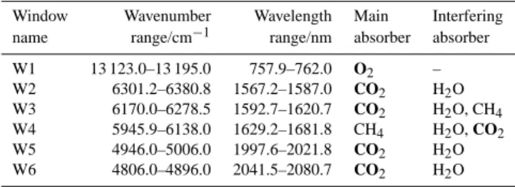
Table 1. Definition of spectral windows used in this study. Boldface indicates target absorbers for the retrieval algorithm.

Window Wavenumber Wavelength Main Interfering name range/cm−1 range/nm absorber absorber W1 13 123.0–13 195.0 757.9–762.0 O₂ – W2 6301.2–6380.8 1567.2–1587.0 CO2 H2O W3 6170.0–6278.5 1592.7–1620.7 CO2 H2O, CH4 W4 5945.9–6138.0 1629.2–1681.8 CH₄ H₂O, CO₂ W5 4946.0–5006.0 1997.6–2021.8 CO₂ H₂O W6 4806.0–4896.0 2041.5–2080.7 CO₂ H₂O

wavelength (up to cubic order). Polarization effects are ne-glected.

Retrieval parameters are the 4-layer partial column pro-files of the target absorbers O2 and CO2, the total column concentrations of other interfering absorbers, spectral shift parameters (per window), and three parameters (per window) driving the Lambertian part of surface reflection. In the O2 A-band, we further fit a radiance offset parameter to account for non-linearity of the detector electronics (Kuze et al., 2012). Surface wind speed, temperature and pressure profiles are not retrieved but interpolated from the meteorological fields. The absorber concentrations to be retrieved are defined per win-dow (Table 1), implying that the retrieval is free to find dif-ferent concentrations for the same chemical species retrieved from different windows. This implies that the derivatives of the forward model with respect to the retrieval parameters are uncoupled among the retrieval windows, i.e. each retrieval parameter corresponds to non-zero Jacobians in exactly one fit window.

Given forward-modelled radiances, an inverse method es-timates the retrieval parameters from the measurements. The inverse method used here is based on a Phillips–Tikhonov scheme which minimizes a cost function composed of two terms. The least-squares term contains the (squared) error-weighted mismatch between measured and modelled radi-ances. The side-constraint term is the first-order finite dif-ference operator for the partial column profiles of the tar-get absorbers and vanishes for all other retrieval parameters. The regularization parameter weighting the side-constraint against the least-squares term is chosen such that each ab-sorber vertical profile gets one degree of freedom. Thus, the inverse method yields absorber profiles with the same shape as the a priori profiles while the total column absorber con-centration is only constrained by the least-squares term.

2.2 Simulation method

For generating simulated measurements, we use the standard variant of RemoTeC which takes into account particle scat-tering in the atmosphere. In order to limit the number of simulations to typical cases, we select one aerosol and one cirrus particle type. The aerosol particles are weakly absorb-ing with sizes followabsorb-ing a bimodal log-normal distribution

with a dominating coarse mode. Assuming sphericity of the aerosols, optical properties are calculated from Mie theory. The cirrus particles are a mixture of randomly oriented planar and columnar crystals with sizes between 0.003 and 1.3 mm (for the longest side). Their optical properties are modelled by the ray-tracing code of Hess (1998). The simulations as-sume generic height distributions of the scattering particles in the atmosphere characterized through the centre height zs and the width wz (full width at half maximum) of a Gaus-sian or a box-like distribution. As for the retrieval method, the simulations treat reflection from the ocean-glint spot by a wind speed-driven Cox-and-Munk reflection model. In sim-ulated ocean-glint geometry, the viewing zenith angle equals exactly the solar zenith angle and the relative solar and view-ing azimuth is zero. Instrument properties such as spectral sampling and instrument line shape are taken from the analy-sis of actual TANSO-FTS spectra. Simulations are performed noiselessly.

2.3 Measurements

Radiances submitted to the retrieval algorithm are either sim-ulated spectra as described above or spectra recorded by the TANSO-FTS onboard GOSAT. The TANSO-FTS ob-servations exploited here are spectra of sunlight backscat-tered from the ocean surface in ocean-glint geometry. We use the ocean-glint criterion defined by Wunch et al. (2011b) to identify suitable scenes. Ocean-glint observations are a regu-larly scheduled operation pattern when GOSAT flies over the ocean. TANSO-FTS records radiances in three SWIR spec-tral bands and, for each band, in two orthogonal polariza-tion direcpolariza-tions, from which we calculate the total backscat-tered radiance according to Yoshida et al. (2011). Instrument line shape and radiometric calibration are provided through GOSAT’s instrument support with recent updates e.g. by Kuze et al. (2012) and Yoshida et al. (2012). The standard measurement sets used here are TANSO-FTS spectra gen-erated by the level 1 processor version 141.141 and later. A sensitivity study in Sect. 4 uses level 1 versions older than 141.141 (version 130.130 and older) in order to illus-trate the usefulness of ocean-glint observations for diagnos-ing errors in the level 1 processor.

3 O2A-band retrieval simulations

The simulations aim at showing that, following the ratio-nale outlined in Sect. 1, the upper edge of [O2] retrievals are indeed scenes where lightpath modification due to light scattering by particles is negligible. To this end, we per-form non-scattering [O2] retrievals from simulated ocean-glint observations of the O2A-band (W1 in Table 1). Aben et al. (2007) performed similar simulations for retrievals of the CO2 total column concentration ([CO2]) from synthetic ocean-glint and land-nadir measurements of the Scanning

Fig. 2. Simulated ratio of retrieved ([O2]) and true O2([O2,true])

total column concentration for various particle optical thicknesses

τ_s (at the O2 A-band). Scenarios cover a coarse particle aerosol

layer in the lower atmosphere (upper panel, Gaussian, zs= 1 km,

w_z= 2 km) and an elevated layer of cirrus particles (lower panel, Gaussian, zs = 10 km, wz= 2 km). Simulations are performed for wind speeds of 2, 5, and 10 m s−1 (red squares, black dots, blue crosses). In the case of 5 m s−1wind speed, retrievals are shown for a solar zenith angle of 5, 15, and 45◦(dotted, solid, dashed lines), which covers the SZA range of 5 to 30◦typical for GOSAT ocean-glint observations.

Imaging Absorption Spectrometer for Atmospheric Cartog-raphy (SCIAMACHY) in the weakly absorbing CO2 band around 6350 cm−1 (similar to W2 in Table 1). They found that the neglect of aerosol and cirrus scattering effects yields underestimation of the true [CO2] for all considered ocean-glint scenarios. For Lambertian land surfaces, however, over-estimation of the true CO2concentration due to unaccounted lightpath enhancement is the usual case for moderate to high surface albedo.

Figure 2 illustrates the effect of the non-scattering as-sumption on retrieved [O2] if scattering particles are present in the atmosphere. The test scenarios cover aerosols in the lower troposphere (Gaussian layer, zs= 1 km, wz= 2 km) and cirrus particles in the upper troposphere (Gaussian layer, zs= 10 km, wz= 2 km). Simulations were performed for a range of particle optical thickness (τs, given at the O2 A-band), solar zenith angle (SZA), and surface wind speed.

The simulations confirm that for the considered aerosol and cirrus scenarios retrieved [O2] increasingly underesti-mates the true concentration with increasing particle optical thickness. Due to the elevated altitude, the cirrus layer has a more severe screening effect than the low-altitude aerosol

layer. Higher wind speed roughens the ocean surface and reduces the amount of directly reflected sunlight. Thus, the contribution of scattered light and the penalty for neglecting scattering in the retrieval generally becomes larger for higher wind speeds. The effect of the solar zenith angle in particular depends on the details of the scattering phase function, which is driven by particle type and size. In accordance with our in-troductory argument, overestimation of the true O2 concen-tration does not occur for these simple generic simulations.

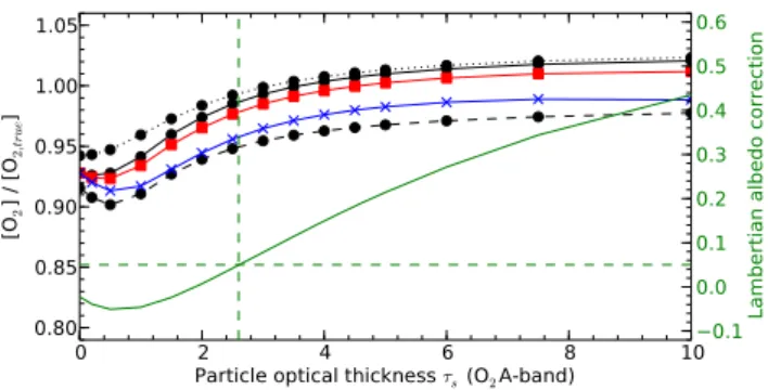
Overestimation of true [O2] could occur in a scenario where an optically thick particle layer at very low altitude is overlaid by an elevated optically thin scattering layer. The lower layer acts as a bright reflector and due to its low alti-tude only shields a small fraction of the O2 column. Mul-tiple scattering between the upper and the lower particle layer could result in a net lightpath enhancement. In that case, retrieved [O2] could overestimate the expected con-centration. Figure 3 illustrates such a scenario. It assumes a double layer of low-altitude particles (box layer) overlaid by a high-altitude cirrus layer (Gaussian layer, zs= 10 km, wz= 2 km) with small optical thickness of τcir= 0.2. If opti-cal thickness of the lower layer is small, the shielding effect of the particle layers dominates, causing severe underestima-tion of the true [O2]. With increasing optical thickness of the lower layer, however, multiple scattering between the lay-ers and, for large optical thickness, multiple scattering within the lower layer itself tend to offset the screening effect. This leads to [O2]/[O2,true] exceeding 1 for large particle optical thickness. The geometric extent of the lower particle layer controls the magnitude of the screening effect and, thus, the amount of multiple scattering events necessary to offset the overall screening.

Thus, there are cases conceivable where a combination of low clouds and elevated scattering layers could result in seemingly accurate or even high-biased [O2] ocean-glint re-trievals. This contradicts the general applicability of the pro-posed method. In order to avoid scenes with multiple scat-tering layers contaminating our findings from GOSAT, we attempt screening such scenes using two criteria. The first criterion is based on the retrieved Lambertian albedo cor-rection (0th order) to the wind speed-driven Cox-and-Munk glint reflection model. Figure 3 shows that for large optical thickness of the lower scattering layer the correction term becomes large as well. Putting an upper limit of 0.05 on the retrieved Lambertian term screens all the simulated scenes, which could contaminate the upper-edge ensemble. The sec-ond screening criterion discards observations contaminated by thin cirrus clouds, similar to the test proposed by Yoshida et al. (2011). The latter screening method exploits the op-tically thick water vapour (H2O) absorption band around 5160 cm−1.

Lambertian

albedo

correction

Fig. 3. Similar to Fig. 2 but for a double layer of low-altitude aerosols with variable optical thickness (τs= 0 to 10) overlaid by a cirrus layer (Gaussian, zs= 10 km, wz= 2 km) of small optical thickness (τcir= 0.2). The geometric extent of the low-layer aerosol

is assumed box-like, extending from the ground to 200, 500, and 800 m (black dots, red squares, blue crosses) altitude. Simulated re-trievals are performed for wind speed of 5 m s−1. For the case of 200 m geometric extent of the lower layer, simulations cover a so-lar zenith angle of 5, 15, and 45◦(dotted, solid, dashed lines). For the latter case with a solar zenith angle of 15◦, the retrieved Lam-bertian albedo correction (green solid line, 0th order term) is shown on the right (green) ordinate scale. Horizontal and vertical dashed green lines illustrate the threshold used for screening contaminated TANSO-FTS scenes.

4 TANSO-FTS O2A-band

The retrieval simulations in Sect. 3 confirm our mechanistic understanding of radiative transfer in ocean-glint geometry. In the next step, we process TANSO-FTS spectra recorded in ocean-glint geometry between June 2009 and Septem-ber 2012 by the non-scattering method. As for the simula-tions, the target quantity is the [O2]/[O2,meteo] ratio. The non-scattering retrievals are subject to some basic quality filters which check for anomalies of the TANSO-FTS instrument, non-convergence of the algorithm, bad quality of the spectral fit (χ2>4) and cirrus contamination.

Figure 4 shows a time series of the [O2]/[O2,meteo] ratio. The retrievals are binned in ∼ 10–12-day clusters, which are separated by ∼ 1–3 days for which GOSAT did not conduct ocean-glint measurements. These temporal bins are selected manually since the operation pattern is not entirely regu-lar. For each of the temporal bins, we generate an occur-rence count similar to Fig. 1 by counting the occuroccur-rence of [O2]/[O2,meteo] values in 0.002 wide slots and normalize it such that a value of 1 indicates the slot with most counts.

As for Fig. 1, we find that overall there is a cloud of low-biased [O2] retrievals bound by a relatively sharp upper edge. In contrast to Fig. 1, the retrievals shown here consider Rayleigh scattering by molecules and use a narrower O2 A-band retrieval window (Table 1). In order to identify the up-per edge, we select all retrievals between the 95th and 99th percentile of [O2] retrievals, separately for each 10–12-day temporal bin. Applying the double-layer filter developed in

Fig. 4. Time series of the [O2]/[O2,meteo] ratio as found by non-scattering retrievals from TANSO-FTS measurements between June 2009

and September 2012 (level 1 version 141.141 and higher). The colour code illustrates the normalized occurrence of retrievals per 10–12-day abscissa (temporal) bin and 0.002 ordinate ([O2]/[O2,meteo] ratio) bin. For each temporal bin, the occurrence is normalized such that the ratio

bin with most counts has a normalized occurrence of 1. We call the “upper edge” all soundings between the 95th and 99th percentile for each temporal bin. The median value within the upper edge is shown as a grey circle. White colour indicates no data.

old L1B version 1

1

1 standard

Fig. 5. Time series of the upper-edge [O2]/[O2,meteo] ratio. Standard non-scattering retrievals (upper panel, level 1 version 141.141 and

later) are compared to retrievals from old level 1 versions (lower panel, version 130.130 and older). Individual soundings are shown as grey squares. Red crosses indicate the median per 10–12-day temporal bin.

Sect. 3 as a final screening step, it rejects 4.3% of the upper-edge data.

Butz et al. (2011) used a different upper-edge criterion based on the retrieval noise error, which worked well for the considered 3-month period. Here, we examine an extended time series and aim at determining the upper edge per 10– 12 day-bin in order to assess temporal variability. The noise criterion failed to determine a reasonable upper edge for sev-eral of the bins. Therefore, we decided to use a conceptually very simple criterion based on ad hoc chosen percentiles. The ambiguity related to the definition of the upper edge is to be considered as part of the intrinsic uncertainty of the method. Most conclusions elaborated on below are not sensitive to the exact choice of the upper edge.

Further, our method can only work if the ensemble from which the upper edge is selected contains a suf-ficient number of clean scenes. When using the 95th-to-99th-percentile range here, we assume that at least these 4 % of the (prescreened) soundings can be con-sidered clean within each temporal bin of 10–12 days over GOSAT’s geographic sampling range. Since our

prescreening preferentially removes scattering-contaminated soundings this seems a safe assumption. If the method is to be applied to spatially small regions and short periods of time, however, care must be taken to allow for a sufficient number of clean cases.

Generally, the upper edge in Fig. 4 does not align with the expected O2concentration at a ratio [O2]/[O2,meteo] = 1 but a factor 1.03 to 1.04 to higher values. The latter finding has been detected previously by Butz et al. (2011) from the first three months of the time series, though Butz et al. (2011) find the upper edge at slightly lower values around 1.030. There, it was suggested to introduce a scaling factor for the line strengths of O2 absorption lines. Differences between this study and Butz et al. (2011) are due to a narrower O2 retrieval window here and due to a different definition of the upper-edge ensemble.

Figure 5 shows the selected upper-edge ensemble of stan-dard retrievals together with the same ensemble reprocessed using spectra generated by older versions of the level 1 pro-cessor (level 1 version 130.130 and older). The latter are only available up to December 2012. Beside the overall scaling

factor, Fig. 5 shows substantial temporal variability of the upper edge of both the standard retrievals as well as the re-trievals from old level 1 versions. The abrupt increase of the latter in April 2011 coincides with the update of the TANSO-FTS level 1 processor to version 130.130, which includes an erroneous correction algorithm for residual non-linearity of the O2A-band detector module (Kuze et al., 2012). The attempted correction in particular results in an undesired change of the instrument line shape (ILS). Since this was unforeseen, [O2] retrievals from level 1 version 130.130 suf-fer from an erroneous ILS model. The new level 1 versions (141.141 and later) clearly remedy this effect.

We find further temporal variability which, so far, cannot be attributed unambiguously to instrumental effects. In par-ticular, the first year of the time series reveals a bowl-shape pattern that rather abruptly ends in August 2010. On 10 Au-gust 2010, the GOSAT team switched on the image motion compensation (IMC) mechanism for ocean-glint operations. IMC makes the TANSO-FTS stare at the same ground spot during the ∼ 4 s acquisition time of the interferogram. Be-fore August 10, 2010, ocean-glint operations were conducted with a fixed pointing mirror orientation making the ground spot move along with the satellite track. Given the apparent effect of the IMC on our upper-edge O2retrievals, one might speculate about slightly erroneous pointing information or its erroneous treatment by the retrieval algorithm before 10 Au-gust, 2010.

So far, the discussion assumes that the upper edge is only affected by time-dependent effects. However, GOSAT’s ocean-glint observation pattern varies seasonally, with denser coverage in the Northern Hemisphere during boreal summer and denser coverage in the Southern Hemisphere during bo-real winter. Therefore, temporal and spatial variability are en-tangled. Seasonal variability of the upper edge, for example, could be caused by a truly seasonal pattern or by a latitudinal pattern that appears time-dependent due to the seasonal cov-erage. We observe some seasonal variation when restricting the selection of the upper-edge ensemble to narrower lati-tude bands, though care must be taken to avoid persistently cloud-covered regions. We will investigate dependencies on latitudes and other parameters such as viewing geometry in forthcoming studies. Short-term effects such as changes in level 1 version and ocean-glint operation pattern should not be affected by spatial variability.

5 TANSO-FTS CO2bands

Section 4 describes how we select the upper edge and use it for testing our forward model of the TANSO-FTS O2 A-band observations. Here, we investigate whether our forward model allows for consistent retrievals of the CO2total col-umn concentration ([CO2]) from different CO2 absorption bands covered by the TANSO-FTS. To this end, we reprocess the upper-edge ensemble by the non-scattering method and

retrieve [CO2]i as a target absorber separately from window Wi with i = 2, 3, 4, 5, 6. As emphasized in Sect. 2, the method is set up such that the windows are uncoupled and [CO2]i re-trieved from one window is free to vary independently from the other windows. If the forward model of the considered windows is consistent, we expect retrieved [CO2]inot to vary among the windows, since the upper-edge ensemble should be free of (wavelength-dependent) particle scattering effects. Figure 6 shows the relative difference of [CO2] retrievals from windows W3, W4, W5, and W6 with respect to the re-trievals from window W2, defined as

1[CO2]i = [CO2]i [CO2]2

− 1, (1)

with i = 3, 4, 5, 6. We find that on average W3 and W6 re-trievals are different from W2 by 0.33 % (1.3 ppm out of 390 ppm) and 0.17 % (0.7 ppm out of 390 ppm), respectively. W4 and W5 retrievals show larger average differences of 1.57 % (6.2 ppm out of 390 ppm) and 2.22 % (8.7 ppm out of 390 ppm) with respect to W2. No systematic temporal pattern is detectable. Variability is dominated by data scatter, which, for W3 and W4, can be explained by the retrieval noise error calculated via error propagation from the out-of-band noise of the TANSO-FTS spectra. For W5 and W6, retrieval noise amounts to roughly half of the observed standard deviation, which could point to some residual scattering effects contam-inating our selection of the upper edge.

The observed differences in [CO2]i could merely reflect sensitivity differences between the individual retrievals. Ver-tical sensitivity of the total column retrieval from window Wi is typically described by the column averaging kernel ai (Rodgers, 2000; Connor et al., 2008). Typical column aver-aging kernels for the various retrieval windows are shown in Fig. 7. The column averaging kernels have a very similar shape for W2 and W3, and for W5 and W6 since the respec-tive bands contain very similar absorption structures of CO2. Thus, we expect the sensitivity effect to be smallest when comparing W2 with W3 and W5 with W6. In fact, Fig. 6 indi-cates that there are differences between W5 and W6 that are larger than differences between W5 and W2. Consequently, the observed difference between W5 and W6 is most likely not attributable to sensitivity effects alone.

In order to assess the effect of different ai on our com-parison of [CO2]i retrieved from the various windows, we estimate the smoothing effects by calculating

1s[CO2]i = a_ix_a a₂x_a

− 1, (2)

where i = 3, 4, 5, 6 and xa is the a priori CO2vertical pro-file derived from CarbonTracker as noted in Sect. 2. Similar to Fig. 6, 1s[CO2]i is then plotted for the upper-edge en-semble and each window (not shown for conciseness). As expected, we find the smallest sensitivity effect when com-paring W2 and W3, amounting to average [CO2] differences of 0.002 %. The greatest [CO2] sensitivity difference is found

-2 0 2 (W 3/W 2-1 )/% 0 33% 0 33% 0 3 % 0 33% -2 0 2 4 6 (W 4/W 2-1 )/% 1 % 1 6% 1 0 % 0 3% 0 2 4 (W 5/W 2-1 )/% 2 22% 2 2 % 0 6 % 0 32% 200/11 2010/0 5 2010/1 1 2011/0 5 2011/1 1 2012/0 5 -2 0 2 (W 6/W 2-1 )/% 0 1 % 0 1 % 0 62% 0 26%

Fig. 6. Relative difference between [CO2] retrieved from various windows. Retrievals from window 3 (uppermost panel, W3), window 4

(upper middle panel, W4), window 5 (lower middle panel, W5), and window 6 (lowermost panel, W6) are referenced to retrievals from window 2 (W2). Individual soundings are shown as grey squares. Red crosses indicate the median per 10–12-day temporal bin. For each panel, the mean difference (1), median difference ( ˆ1), standard deviation of differences (σ ), and the average retrieval noise error ( ˆσ) are given in percent.

between W2 and W5, W6 retrievals, with an average dif-ference of 0.17 %. Average sensitivity difdif-ferences between W2 and W4 amount to 0.10 %. The averaging kernels ai ex-hibit some temporal variability due to observation geome-try, signal-to-noise, and concentration distributions changing over time. Thus, 1s[CO2]i also exhibits a time dependence, the amplitude of which is typically on the order of the ob-served average differences.

Considering the magnitude of the effect of retrieval sen-sitivity on [CO2]i, we conclude that the agreement found for our ocean-glint CO2 retrievals from W2, W3, and W6 is within the range which could be affected by sensitivity is-sues. Strictly, the detected mean difference between W2 and W3 retrievals of 0.33 % is significantly greater than the ef-fect expected from sensitivity differences (less than 0.01 %), so we are tempted to attribute this small difference to an ac-tual shortcoming of the input data to our algorithm. CO2 re-trievals from W4 and W5, however, show large differences when compared to retrievals from W2, W3, and W6. These differences greatly surpass the effect expected from different

averaging kernels. Our forward model for W4 and W5 must suffer from an inconsistency that causes this pattern.

The obvious candidate for such an inconsistency is the calibration of the absorption line strengths among the vari-ous CO2retrieval windows. The use of erroneous instrument line shape functions would be another candidate that could cause these inconsistent CO2retrievals. The latter seems un-likely since all CO2windows are extracted from band 2 and band 3 of the TANSO-FTS SWIR observations, which ex-hibit accurate knowledge of the instrument line shape. For W4, we note a strong dependence of retrieved [CO2]4on the polynomial order of the albedo correction. Since we are not able to unambiguously determine the root cause for this al-gorithm deficiency, we recommend not using W4 and W5 together with W2, W3 or W6 for CO2 retrievals or to un-couple W4 and W5 from W2, W3 and W6 when setting up the retrieval method. Alternatively, we will consider a similar strategy as for our O2A-band forward model, where we pro-posed to scale the O2absorption line strengths by a constant factor to make the O2A-band forward model consistent with

0.4 0.6 0.8 1.0 1.2 1.4 1.6 Column averaging kernel

100 200 300 400 500 600 700 800 900 W2 W3 W4 W5 W6

Fig. 7. Column averaging kernels for [CO2] retrieved from

win-dows W2 (black solid squares), W3 (black open squares), W4 (red solid circles), W5 (blue solid diamonds), and W6 (blue open dia-monds). Averaging kernels for W2 and W3 are almost indistinguish-able. For each window, the mean column averaging kernel among the upper-edge ensemble is shown.

meteorological surface pressure. For CO2retrievals from W2 through W6, one could introduce similar scaling factors to make the forward model consistent among the various win-dows.

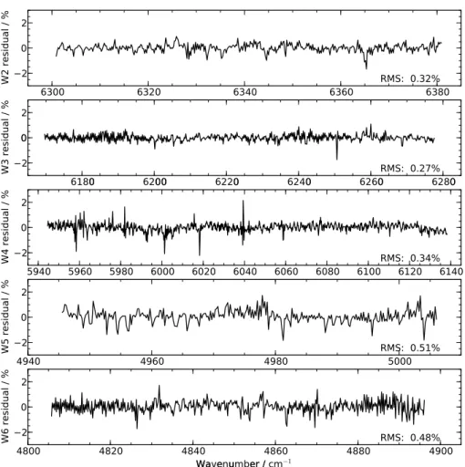
Going beyond the assessment of line strengths, line shape errors can be investigated by evaluating the quality of the spectral fit. Figure 8 shows the relative fitting residuals among the upper-edge soundings for the year 2010. The residuals are calculated by dividing the difference between measured and fitted spectrum by the continuum radiance in each window. Following our rationale that the upper-edge en-semble is not affected by unaccounted scattering effects, the residuals in Fig. 8 are dominated by systematic errors of the spectroscopic parameters or by deficiencies of the employed line shape models. Clearly, line shape calculation seems most challenging in windows W5 and W6, which cover strong CO2(and H2O) absorption lines. Here, we employ the line-mixing model of Lamouroux et al. (2010) for calculating the CO2absorption line shape. Figure 8 indicates that even more subtle line shape effects might need to be considered for the strongly absorbing CO2bands (Thompson et al., 2012).

6 Conclusions and discussion

Observations of sunlight backscattered from the glint spot on the ocean surface offer a tool to select an ensemble of observations that do not suffer from errors due to un-certain knowledge of the lightpath. Since lightpath modi-fication by atmospheric particles in general is a dominat-ing source of uncertainty for the retrieval of atmospheric

constituent concentrations from solar backscatter measure-ments, our method allows for assessing other sources of error often masked by lightpath-related errors.

We suggest to identify the ensemble by performing [O2] retrievals from ocean-glint spectra of the O2 A-band. Re-trievals are performed under the assumption of negligible particle scattering in the atmosphere and, thus, are compu-tationally cheap. Simulations confirm that light scattering by particles is negligible for the upper edge of these retrievals, i.e. the retrievals which show the least underestimation with respect to [O2,meteo], the O2concentration expected from me-teorological support data. A caveat applies for scenes where an optically thick particle layer such as a cloud at low altitude acts as a bright reflector and is overlaid by an optically thin elevated scattering layer such as cirrus. Independent cloud screening can help avoid contamination of the upper-edge ensemble by such scenes.

For real measurements such as from the TANSO-FTS on-board GOSAT, selection of the upper edge to some extent de-pends on the identification criterion. Here, we use a concep-tually very simple criterion attributing soundings to the upper edge which yield 95 to 99 % of the largest [O2]/[O2,meteo] ra-tios. Further uncertainty is introduced by the meteorological and geolocation data which are used to calculate [O2,meteo] for each sounding. Case studies have shown that ECMWF surface pressure used here for meteorological input is accu-rate to a few hPa (King, 2003; Lammert et al., 2008).

We derive the upper-edge ensemble for 10–12-day periods over more than 3 yr of TANSO-FTS ocean-glint observations between June 2009 and September 2012. The correspond-ing [O2]/[O2,meteo] ratios do not align at the expected ratio of unity but at a ratio of 1.03 to 1.04, which largely confirms findings by our precursor study (Butz et al., 2011). There, we speculated on a potential scaling factor of 1.030 to be applied to the O2line strengths in the O2A-band. Crisp et al. (2012) derive a similar scaling factor of 1.025 based on their sur-face pressure retrievals from TANSO-FTS nadir-land obser-vations. Given the uncertainty in determining the upper edge by our method, the findings by Crisp et al. (2012) and Butz et al. (2011) appear consistent. Yoshida et al. (2013) find a smaller scaling factor of 1.010 using the upper-edge method and Cogan et al. (2012) conclude on a surface pressure bias of only 4 hPa when not scaling the O2line strengths. Clearly, findings on a potential spectroscopic scaling factor depend on the spectroscopic parameters used to drive the retrieval forward models, which might not be identical among dif-ferent retrieval methods. Nevertheless, an inconsistency be-tween the former and latter studies remains.

The upper-edge [O2]/[O2,meteo] ensemble obtained by pro-cessing the most recent TANSO-FTS level 1 spectra (ver-sion 141.141 and later) reveals a substantial time dependence in particular in the first year of the mission. An abrupt change of the [O2]/[O2,meteo] ratios coincides with activation of the image motion compensation for ocean-glint observations in August 2010. After August 2010, time dependencies are

W2 residual / % RMS: 0.32% 0 200 220 2 0 2 0 2 0 2 0 2 W3 residual / % RMS: 0.27% 0 0 0 000 020 0 0 0 0 0 0 00 20 0 2 0 2 W4 residual / % RMS: 0.34% 4 40 4 0 4 0 000 2 0 2 W5 residual / % RMS: 0.51% 4 00 4 20 4 40 4 0 4 0 4 00 Wa e u er / 2 0 2 W6 residual / % RMS: 0.48%

Fig. 8. Fitting residuals for windows W2 (upper panel), W3 (second panel), W4 (third panel), W5 (fourth panel), and W6 (lower panel) relative to the continuum radiance. We average all 4518 upper-edge soundings in the year 2010 such that the residuals are dominated by systematic errors. The residual root mean square (RMS) is quoted at the lower right of each panel.

small. For an older level 1 dataset (version 130.130), the [O2]/[O2,meteo] ratios clearly monitor the detrimental im-pact of an erroneous non-linearity correction scheme on con-stituent retrievals.

We further use the upper-edge ensemble to conduct [CO2] retrievals from several absorption bands covered by the TANSO-FTS and to be covered by future satellite missions. The CO2concentrations found are consistent to better than 1.5 ppm among the bands (W2, W3, W6: around 6350, 6200, 4850 cm−1, respectively) which are heavily used for CO2 retrievals from TANSO-FTS, the upcoming Orbiting bon Observatory (OCO-2), and the ground-based Total Car-bon Column Observing Network (TCCON) (Wunch et al., 2011a). Considerable effort has been put into determining the related spectroscopic parameters with high accuracy (e.g. Lamouroux et al., 2010; Devi et al., 2010). Substantially larger retrieval differences are observed for two other CO2 absorption bands (W4, W5: around 6000, 4970 cm−1), point-ing to errors in the spectroscopic line strength parameters. The detected inconsistencies are unacceptably large in view of the stringent accuracy requirements for remote sensing of

CO2concentrations and, thus, demand further investigation if these bands are to be used for monitoring of CO2or for si-multaneous use with the other bands. Examining the spectral fitting residuals shows that line shape errors are most pro-nounced for the strongly absorbing CO2 bands (W5, W6: around 4970, 4850 cm−1).

Acknowledgements. AB is supported by Deutsche Forschungsge-meinschaft (DFG) through the Emmy-Noether programme, grant BU2599/1-1 (RemoteC). Access to GOSAT data was granted through the 2nd GOSAT research announcement jointly issued by JAXA, NIES, and MOE. ECMWF ERA Interim analyses are pro-vided through http://data-portal.ecmwf.int/data/d/interim_daily/. CarbonTracker data are provided by NOAA ESRL, Boulder, Col-orado, USA from the Web site at http://carbontracker.noaa.gov. We acknowledge support by Deutsche Forschungsgemeinschaft and Open Access Publishing Fund of Karlsruhe Institute of Technology. The service charges for this open access publication

have been covered by a Research Centre of the Helmholtz Association.

References

Aben, I., Hasekamp, O., and Hartmann, W.: Uncertainties in the space-based measurements of CO2columns due to scattering in

the Earth’s atmosphere, J. Quant. Spectrosc. Ra., 104, 450–459, doi:10.1016/j.jqsrt.2006.09.013, 2007.

Butz, A., Guerlet, S., Hasekamp, O., Schepers, D., Galli, A., Aben, I., Frankenberg, C., Hartmann, J.-M., Tran, H., Kuze, A., Keppel-Aleks, G., Toon, G., Wunch, D., Wennberg, P., Deutscher, N., Griffith, D., Macatangay, R., Messerschmidt, J., Notholt, J., and Warneke, T.: Toward accurate CO2 and CH4

observations from GOSAT, Geophys. Res. Lett., 38, L14812, doi:10.1029/2011GL047888, 2011.

Butz, A., Galli, A., Hasekamp, O., Landgraf, J., Tol, P., and Aben, I.: TROPOMI aboard Sentinel-5 Precursor: Prospec-tive performance of CH4 retrievals for aerosol and cirrus

loaded atmospheres, Remote Sens. Environ., 120, 267–276, doi:10.1016/j.rse.2011.05.030, 2012.

Cogan, A. J., Boesch, H., Parker, R. J., Feng, L., Palmer, P. I., Blavier, J.-F. L., Deutscher, N. M., Macatangay, R., Notholt, J., Roehl, C., Warneke, T., and Wunch, D.: Atmospheric carbon dioxide retrieved from the Greenhouse gases Observing SATel-lite (GOSAT): Comparison with ground-based TCCON obser-vations and GEOS-Chem model calculations, J. Geophys. Res., 117, D21301, doi:10.1029/2012JD018087, 2012.

Connor, B. J., Bösch, H., Toon, G., Sen, B., Miller, C., and Crisp, D.: Orbiting Carbon Observatory: Inverse method and prospective error analysis, J. Geophys. Res., 113, 5305, doi:10.1029/2006JD008336, 2008.

Cox, C. and Munk, W.: Statistics of the sea surface derived from sun glitter, J. Mar. Res., 13, 198–227, 1954.

Crisp, D., Atlas, R. M., Bréon, F.-M., Brown, L. R., Burrows, J. P., Ciais, P., Connor, B. J., Doney, S. C., Fung, I. Y., Jacob, D. J., Miller, C. E., O’Brien, D., Pawson, S., Randerson, J. T., Rayner, P., Salawitch, R. J., Sander, S. P., Sen, B., Stephens, G. L., Tans, P. P., Toon, G. C., Wennberg, P. O., Wofsy, S. C., Yung, Y. L., Kuang, Z., Chudasama, B., Sprague, G., Weiss, B., Pollock, R., Kenyon, D., and Schroll, S.: The Orbiting Car-bon Observatory (OCO) mission, Adv. Space Res., 34, 700–709, doi:10.1016/j.asr.2003.08.062, 2004.

Crisp, D., Fisher, B. M., O’Dell, C., Frankenberg, C., Basilio, R., Bösch, H., Brown, L. R., Castano, R., Connor, B., Deutscher, N. M., Eldering, A., Griffith, D., Gunson, M., Kuze, A., Man-drake, L., McDuffie, J., Messerschmidt, J., Miller, C. E., Morino, I., Natraj, V., Notholt, J., O’Brien, D. M., Oyafuso, F., Polonsky, I., Robinson, J., Salawitch, R., Sherlock, V., Smyth, M., Suto, H., Taylor, T. E., Thompson, D. R., Wennberg, P. O., Wunch, D., and Yung, Y. L.: The ACOS CO2retrieval algorithm – Part II: Global X_CO2 data characterization, Atmos. Meas. Tech., 5, 687–707, doi:10.5194/amt-5-687-2012, 2012.

Devi, M. V., Benner, D. C., Miller, C. E., and Predoi-Cross, A.: Lorentz half-width, pressure-induced shift and speed-dependent coefficients in oxygen-broadened CO2 bands at 6227 and

6348 cm−1using a constrained multispectrum analysis, J. Quant. Spectrosc. Ra., 111, 2355–2369, 2010.

Hasekamp, O. P. and Butz, A.: Efficient calculation of intensity and polarization spectra in vertically inhomogeneous scatter-ing and absorbscatter-ing atmospheres, J. Geophys. Res., 113, 20309, doi:10.1029/2008JD010379, 2008.

Hasekamp, O. P. and Landgraf, J.: A linearized vector radiative transfer model for atmospheric trace gas retrieval, J. Quant. Spec-trosc. Ra., 75, 221–238, doi:10.1016/S0022-4073(01)00247-3, 2002.

Hasekamp, O. P. and Landgraf, J.: Linearization of vector ra-diative transfer with respect to aerosol properties and its use in satellite remote sensing, J. Geophys. Res., 110, 4203, doi:10.1029/2004JD005260, 2005.

Hess, M.: Scattering matrices of imperfect hexagonal ice crys-tals, J. Quant. Spectrosc. Ra., 60, 301–308, doi:10.1016/S0022-4073(98)00007-7, 1998.

King, J. C.: Validation of ECMWF Sea Level Pres-sure Analyses over the Bellingshausen Sea, Antarc-tica, Weather Forecast., 18, 536–540, doi:10.1175/1520-0434(2003)18<536:VOESLP>2.0.CO;2, 2003.

Kuze, A., Suto, H., Nakajima, M., and Hamazaki, T.: Ther-mal and near infrared sensor for carbon observation Fourier-transform spectrometer on the Greenhouse Gases Observing Satellite for greenhouse gases monitoring, Appl. Optics, 48, 6716, doi:10.1364/AO.48.006716, 2009.

Kuze, A., Suto, H., Shiomi, K., Urabe, T., Nakajima, M., Yoshida, J., Kawashima, T., Yamamoto, Y., Kataoka, F., and Buijs, H.: Level 1 algorithms for TANSO on GOSAT: processing and on-orbit calibrations, Atmos. Meas. Tech., 5, 2447–2467, doi:10.5194/amt-5-2447-2012, 2012.

Lammert, A., Brümmer, B., Ebbers, I., and Müller, G.: Validation of ECMWF and DWD model analyses with buoy measurements over the Norwegian Sea, Meteorol. Atmos. Phys., 102, 87–96, doi:10.1007/s00703-008-0008-1, 2008.

Lamouroux, J., Tran, H., Laraia, A. L., Gamache, R. R., Rothman, L. S., Gordon, I. E., and Hartmann, J.: Updated database plus software for line-mixing in CO2infrared spectra and their test

using laboratory spectra in the 1.5–2.3 µm region, J. Quant. Spec-trosc. Ra., 111, 2321–2331, doi:10.1016/j.jqsrt.2010.03.006, 2010.

Meirink, J. F., Bergamaschi, P., Frankenberg, C., d’Amelio, M. T. S., Dlugokencky, E. J., Gatti, L. V., Houweling, S., Miller, J. B., Röckmann, T., Villani, M. G., and Krol, M. C.: Four-dimensional variational data assimilation for in-verse modeling of atmospheric methane emissions: Analysis of SCIAMACHY observations, J. Geophys. Res., 113, 17301, doi:10.1029/2007JD009740, 2008.

Miller, C. E., Crisp, D., DeCola, P. L., Olsen, S. C., Randerson, J. T., Michalak, A. M., Alkhaled, A., Rayner, P., Jacob, D. J., Suntharalingam, P., Jones, D. B. A., Denning, A. S., Nicholls, M. E., Doney, S. C., Pawson, S., Bösch, H., Connor, B. J., Fung, I. Y., O’Brien, D., Salawitch, R. J., Sander, S. P., Sen, B., Tans, P., Toon, G. C., Wennberg, P. O., Wofsy, S. C., Yung, Y. L., and Law, R. M.: Precision requirements for space-based XCO2 data, J. Geophys. Res., 112, 10314, doi:10.1029/2006JD007659, 2007.

Peters, W., Jacobson, A. R., Sweeney, C., Andrews, A. E., Con-way, T. J., Masarie, K., Miller, J. B., Bruhwiler, L. M. P., Petron, G., Hirsch, A. I., Worthy, D. E. J., van der Werf, G. R., Ran-derson, J. T., Wennberg, P. O., Krol, M. C., and Tans, P. P.: An atmospheric perspective on North American carbon dioxide ex-change: CarbonTracker, P. Natl. Acad. Sci., 104, 18925–18930, 2007.

Rodgers, C. D.: Inverse Methods for Atmospheric Sounding: The-ory and Practice, World Scientific, River Edge, N.J., USA, 2000. Rothman, L. S., Gordon, I. E., Barbe, A., Benner, D. C., Bernath, P. F., Birk, M., Boudon, V., Brown, L. R., Campargue, A., Cham-pion, J., Chance, K., Coudert, L. H., Dana, V., Devi, V. M., Fally, S., Flaud, J., Gamache, R. R., Goldman, A., Jacquemart, D., Kleiner, I., Lacome, N., Lafferty, W. J., Mandin, J., Massie, S. T., Mikhailenko, S. N., Miller, C. E., Moazzen-Ahmadi, N., Nau-menko, O. V., Nikitin, A. V., Orphal, J., Perevalov, V. I., Perrin, A., Predoi-Cross, A., Rinsland, C. P., Rotger, M., Šimeˇcková, M., Smith, M. A. H., Sung, K., Tashkun, S. A., Tennyson, J., Toth, R. A., Vandaele, A. C., and Vander Auwera, J.: The HITRAN 2008 molecular spectroscopic database, J. Quant. Spectrosc. Ra., 110, 533–572, doi:10.1016/j.jqsrt.2009.02.013, 2009.

Schepers, D., Guerlet, S., Butz, A., Landgraf, J., Frankenberg, C., Hasekamp, O., Blavier, J.-F., Deutscher, N. M., Griffith, D. W. T., Hase, F., Kyro, E., Morino, I., Sherlock, V., Sussmann, R., and Aben, I.: Methane retrievals from Greenhouse Gases Observ-ing Satellite (GOSAT) shortwave infrared measurements: Perfor-mance comparison of proxy and physics retrieval algorithms, J. Geophys. Res., 117, D10307, doi:10.1029/2012JD017549, 2012. Thompson, D. R., Benner, D. C., Brown, L. R., Crisp, D., Devi, V. M., Jiang, Y., Natraj, V., Oyafuso, F., Sung, K., Wunch, D., Castaño, R., and Miller, C. E.: Atmospheric val-idation of high accuracy CO2 absorption coefficients for the

OCO-2 mission, J. Quant. Spectrosc. Ra., 113, 2265–2276, doi:10.1016/j.jqsrt.2012.05.021, 2012.

Tran, H. and Hartmann, J.: An improved O₂ A band absorp-tion model and its consequences for retrievals of photon paths and surface pressures, J. Geophys. Res., 113, 1810, doi:10.1029/2008JD010011, 2008.

Wunch, D., Toon, G. C., Blavier, J.-F. L., Washenfelder, R., Notholt, J., Connor, B. J., Griffith, D. W. T., Sherlock, V., and Wennberg, P. O. W.: The Total Carbon Column Observing Network, Philos. T. Roy. Soc. A, 369, doi:10.1098/rsta.2010.0240, 2011a.

Wunch, D., Wennberg, P. O., Toon, G. C., Connor, B. J., Fisher, B., Osterman, G. B., Frankenberg, C., Mandrake, L., O’Dell, C., Ahonen, P., Biraud, S. C., Castano, R., Cressie, N., Crisp, D., Deutscher, N. M., Eldering, A., Fisher, M. L., Griffith, D. W. T., Gunson, M., Heikkinen, P., Keppel-Aleks, G., Kyrö, E., Lindenmaier, R., Macatangay, R., Mendonca, J., Messerschmidt, J., Miller, C. E., Morino, I., Notholt, J., Oyafuso, F. A., Ret-tinger, M., Robinson, J., Roehl, C. M., Salawitch, R. J., Sher-lock, V., Strong, K., Sussmann, R., Tanaka, T., Thompson, D. R., Uchino, O., Warneke, T., and Wofsy, S. C.: A method for eval-uating bias in global measurements of CO2total columns from

space, Atmos. Chem. Phys., 11, 12317–12337, doi:10.5194/acp-11-12317-2011, 2011b.

Yoshida, Y., Ota, Y., Eguchi, N., Kikuchi, N., Nobuta, K., Tran, H., Morino, I., and Yokota, T.: Retrieval algorithm for CO2and CH4

column abundances from short-wavelength infrared spectral ob-servations by the Greenhouse gases observing satellite, Atmos. Meas. Tech., 4, 717–734, doi:10.5194/amt-4-717-2011, 2011. Yoshida, Y., Kikuchi, N., and Yokota, T.: On-orbit radiometric

cal-ibration of SWIR bands of TANSO-FTS onboard GOSAT, At-mos. Meas. Tech., 5, 2515–2523, doi:10.5194/amt-5-2515-2012, 2012.

Yoshida, Y., Kikuchi, N., Morino, I., Uchino, O., Oshchepkov, S., Bril, A., Saeki, T., Schutgens, N., Toon, G. C., Wunch, D., Roehl, C. M., Wennberg, P. O., Griffith, D. W. T., Deutscher, N. M., Warneke, T., Notholt, J., Robinson, J., Sherlock, V., Connor, B., Rettinger, M., Sussmann, R., Ahonen, P., Heikkinen, P., Kyrö, E., Mendonca, J., Strong, K., Hase, F., Dohe, S., and Yokota, T.: Improvement of the retrieval algorithm for GOSAT SWIR

XCO2and XCH4and their validation using TCCON data,

At-mos. Meas. Tech., 6, 1533–1547, doi:10.5194/amt-6-1533-2013, 2013.