Effect of power amplifier nonlinearity on system performance metric, bit-error-rate (BER)

Effect of Power Amplifier Nonlinearity on

System Performance Metric, Bit-Error-Rate (BER)

by

Farinaz Edalat

Bachelor of Science in Computer Engineering

University of Illinois at Urbana-Champaign, 2001

Submitted to the Department of Electrical Engineering and Computer Science in

Partial Fulfillment of the Requirements for the Degree of

Master of Science in Electrical Engineering and Computer Science

at the

MASSACHUSETTS INSTITUTE OF TECHNOLOGY

September 2003

2003 Massachusetts Institute of Technology. All rights reserved.

Signiture of Author: ...

Depart ent Electrical Engineering and Computer Science

August 29, 2003

Certified by: ...

Charles G. Sodini

Professor of Electrical Engineering and Computer Science

Thesis Supervisor

Accepted by: ...

Arthur C. Smith

Professor of Electrical Engineering and Computer Science

Chairman, Committee for Graduate Students

BARKER

MASSACHUSETS INSTITUTE OF TECHNOLOGY

AT

Effect of Power Amplifier Nonlinearity on

System Performance Metric, Bit-Error-Rate (BER)

by

Farinaz Edalat

Submitted to the Department of Electrical Engineering and Computer Science on August 29, 2003 in Partial Fulfillment of the

Requirements for the degree of

Master of Science in Electrical Engineering and Computer Science

Abstract

In today's high-speed wireless communication applications, the simultaneous demand for bandwidth-efficient modulation schemes such as M-QAM and high power-efficiency of elec-tronic components in the system imposes a contradicting tradeoff. On one hand, with the RF power amplifier (PA) at the transmitter antenna being the major power "hungry" block in many such systems, high power-efficiency for the system is obtained when the PA con-sumes most of the little supplied dc power (e.g. from a battery) as RF power, which is the power delivered to the load. On the other hand, at high powers, the PA becomes nonlinear, which becomes problematic when the input to the PA has a time-varying envelope. More precisely, when an M-QAM modulated signal (which has varying envelope and phase) is transmitted, the PA nonlinearity characteristics adversely affect the system performance, such as degradation of the Bit Error Rate (BER).

Although linearization and compensation techniques can be used to minimize the above mentioned degradation in system performance, such techniques are mostly not suitable for low-cost and small-size integrated-circuit implementations. As a result, to obtain an optimal solution to this linearity/efficiency tradeoff, the objective of this thesis is to qualitatively and quantitatively characterize the effect of the PA nonlinearity on the system performance metric, BER. To gain an intuitive understanding of the effect of the PA nonlinearity, a system simulation is developed. In addition, to achieve a simple relationship between this circuit nonlinearity and system performance, an appropriate model (AM-AM/AM-PM) to characterize the PA nonlinearity is found. In fact, the results of this thesis in characterizing the effect of the PA nonlinearity on system performance can be useful to PA designers to de-sign cost-effective and efficient PAs by finding a PA operating point that lies in the nonlinear region as much as possible while still meeting the system performance requirements. Thesis Supervisor: Charles G. Sodini

Acknowledgments

There are many people that I would like to thank without whom the completion of this thesis would not have been possible.

First and foremost, I would like to express my whole-hearted gratitude to my advisor, Professor Charles Sodini, for his invaluable guidance, insight, and encouragement through-out this thesis work. The experience of mixing the system and circuits spices was truly thrilling!

My special appreciation goes to Professor Michael Perrott whose prompt assistance with using the CppSim simulation tool speeded up my work to a great extend and made experience of working with this tool an enjoyable one. I would also like to thank Professor Muriel Medard for her valuable suggestions on some system issues of this project.

My tremendous thanks go to my officemates, Andy Wang and Anh Pham for their technical support and friendship. Andy was a great teacher in sharing his rich and vast theoretical and practical knowledge in communication systems and circuits as well as simu-lation tools. His ingenious questions and ideas often led me in the right path by making me look at things from a different angle. Anh is who I call the "power amp wiz" to whom I am obliged for much of my understanding of power amplifiers. His countless hours of answering my confusions about circuit theories were precious. I would also like to thank my friend and colleague, Ali Motamedi, for sharing his valuable insights and giving consultations on some power amplifier issues.

My gratefulness is extended to all my other colleagues in the office. I thank Todd Sepke for his assistance with all computing problems. The hot talks on ski adventures and making ski trip plans with John Fiorenza, a truly expert downhill skier, were always inspiring. My thanks go to the rest of the group who inspired me to join the Mallard MTL Hockey team and made the office a fun and comfortable environment to work: Andrew Chen, Albert Chow, Matt Guyton, Lunal Khuon, Jacky Liang, Pablo Acosta-Serafini, and Mark Spaeth.

I would like to thank all my other friends and colleagues for their warmth and laughters that have made MIT a fun place to be. I am especially grateful for the love and encourage-ment of my closest friends, Bahareh Banijamali and Miriam Bruhn (my best roommate as well). In addition, much appreciation goes to MIT's athletics facilities (Dupont gym and the Z-center): those every evening workout helped me to be more effective and energetic for the rest of the day.

I am very grateful to Marilyn Pierce for making the administrative issues and paper works the most time-efficient.

Finally, I would like to thank my family for always being there for me. I thank my fan-tastic sister and brother for their love and support. Thank you mom for your unconditional love and wisdom have helped me survive the difficult times. Dad, your brilliant advice and constant supervision have provided me with confidence and strength to always take one step further and challenge myself. Mom and dad this thesis is dedicated to you.

This work is sponsored, in part, by the National Defense Science and Engineering

Contents

1 Introduction

1.1 Thesis Objective . . . . 1.2 Thesis Outline . . . .

2 Wireless Communications System - Background

2.1 Performance Measurement Metrics . . . . 2.1.1 Bit-Error-Rate (BER) . . . . 2.1.2 Bandwidth . . . . 2.1.3 Power efficiency . . . . 2.2 M odulator . . . . 2.2.1 Quadrature Amplitude Modulation (QAM) . . . . . 2.2.2 Pulse-Shaping (Baseband) Filter . . . . 2.3 C hannel . . . . 2.4 Optimum Receiver . . . . 2.4.1 Demodulator . . . . 2.4.2 Detector (or Decoder) . . . .

3 Power Amplifier Characteristics and Nonlinearity Effects 3.1 Input-Output Characteristics of PA . . . . 3.1.1 Input-Output Characteristics - Linear PA . . . . 3.1.2 Input-Output Characteristics - Nonlinear PA . . . . 3.2 Nonlinearity Effects of PA . . . . 3.2.1 Single-Tone Test . . . . 3.2.2 Two-Tone Test . . . .

4 Simulation

4.1 Simulation Tool . . . . 4.2 System Simulation Component Blocks . . . . 4.2.1 Modulator . . . .

4.2.2 P A . . . . 4.2.3 C hannel . . . .

4.2.4 Demodulator . . . . 4.2.5 D etector . . . . 4.2.6 System Performance Measurement -BER . . . . 4.3 Generality of the System . . . . 4.4 Issues and Challenges in the Simulation . . . . 4.4.1 Real or Complex Signals . . . .

Background 13 14 14 17 18 18 18 19 19 20 23 25 26 26 29 35 35 36 36 41 41 43 47 47 48 49 53 53 54 55 55 57 57 57

4.4.2 Performance of an Ideal System . . . . 58 4.4.3 PA Operating Point . . . . 58 4.4.4 SN R . . . . 59

5 PA Nonlinearity Model 61

5.1 PA Nonlinearity Model: AM-AM/AM-PM ... ... 61 5.2 Specifications of Experimented PA ... ... 63 5.3 Nonlinearity Model of Simulated PA ... ... 63

6 Effect of PA Nonlinearity on System Performance Metric - BER 67 6.1 Literature Background . . . . 67 6.2 Visualization of the Effect of PA Nonlinearity on BER . . . . 68 6.2.1 Effect of PA Nonlinearity Alone . . . . 68 6.2.2 Effect of PA Nonlinearity in a Communications System without AWGN

Channel ... ... 70 6.2.3 Effect of PA Nonlinearity in a Communications System with AWGN

C hannel . . . . 70 6.3 Quantification of the Effect of PA Nonlinearity on BER . . . . 74 6.3.1 Effect of PA Nonlinearity on BER - 16-QAM . . . . 74

6.3.2 Effect of PA Nonlinearity on BER: 16-QAM versus 64-QAM . . . . 77 6.4 Application: Finding the Optimal PA Operating Point . . . . 82

7 Conclusions 85

7.1 Sum m ary . . . . 85 7.2 Future W ork . . . .. . . . . 87

List of Figures

2-1 Basic building blocks of a wireless communications system. . . . . 17

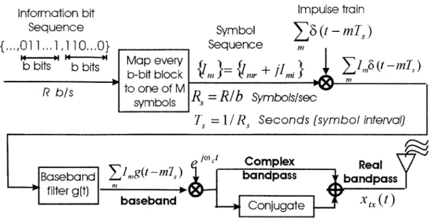
2-2 A complex implementation of the QAM modulation followed by conversion to a real bandpass signal, xtx(t), to be transmitted over the channel. . . . . 21

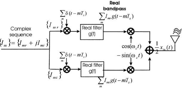
2-3 An alternative realization of QAM modulation in which the real symbol sequences {Imr} and {Imi} are acted upon individually. The final real bandpass signal, xtx (t), is obtained by adding the two real bandpass signals on the quadrature carriers. . . 22

2-4 Gray encoding of a 16-QAM signal constellation. . . . . 22

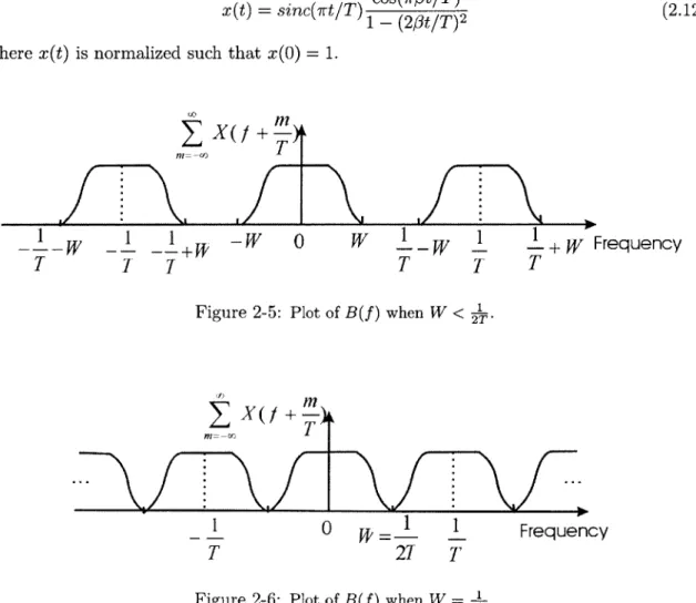
2-5 Plot of B(f) when W < ... . . . .. 24

2-6 Plotof B~f)when W T . . . ... 2

2-6 Plot of B(f) when W 1...24

2-7 Plot of B(f) when W > 1... . . . . 25

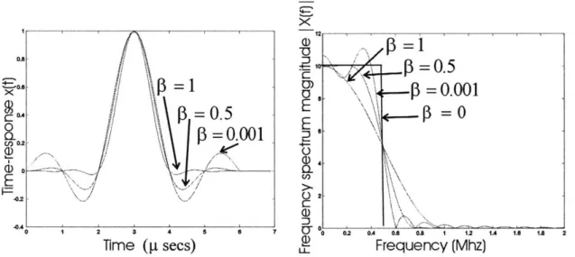
2-8 Effect of the roll-factor on the time response and frequency spectrum of the raised-cosine filter. The time and frequency-domain characteristics are depicted for the roll-off factors = 0.001, 0.5, 1. . . . . 25

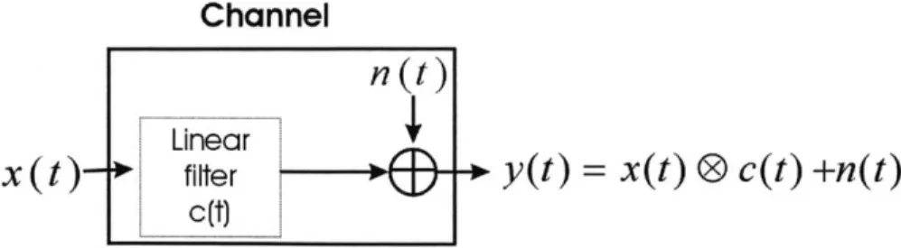
2-9 A model of a band-limited channel: a linear filter with an additive noise. (0 repre-sents the convolution operation.) . . . . 26

2-10 A plot showing the error probability in detecting the corrupted symbol y when al was sent under the MD rule. Since noise

n

> d(ai, a2)/2, it moves the transmitted symbol a1 closer to the other symbol a2, which is thus mistakenly detected as the transmitted symbol. . . . . 30

3-1 Power Amplifier two-port model. . . . . 35

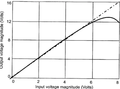
3-2 Input-output voltage characteristics (Source: Pothecary [5]) . . . . 37

3-3 Definition of the 1-dB compression point (Source: Razavi [2]). . . . . 37

3-4 Power amplifier AM-AM characteristic. . . . . 39

3-5 Measured AM-PM for a 1-Watt, 1.9 GHz PA. Circles indicate the 1-dB compression points (Source: Cripps [7]). . . . . 40

3-6 Input and output signals in Saleh's PA Model. . . . . 40

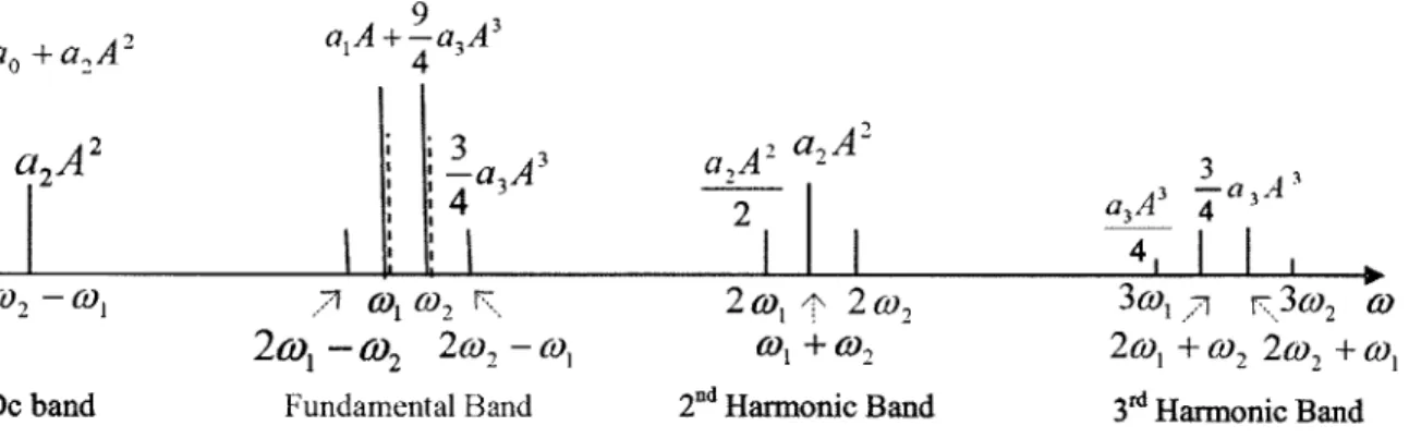
3-7 Effect of the PA nonlinearity: harmonics and intermodulation distortions. . . . . . 43

3-8 Effect of the PA nonlinearity: corruption of a signal due to the intermodulation between two interferers (Source: Razavi [2]). . . . . 44

3-9 Definition of the third-order intercept point IP3 based on the growth of output components in a two-tone test (Source: Razavi [2]). . . . . 44

4-1 High level schematic description of the simulated system. . . . . 48 4-2 _{Plot showing the response of a square-root raised cosine filter (at the transmitter)}

to an impulse train (generated by an M-QAM source), followed by the response of a second square-root raised cosine filter (at the receiver) to the output of the first filter. 51

4-3 The effect of roll-off factor on the response of filter to a sequence of randomly gen-erated data. . . . . 52 4-4 The modulator consists of an M-QAM source and a square-root raised cosine filter.

The M-QAM modulation is a 16-QAM or 64-QAM with Gray encoding mapping and a rectangular constellation. The QAM source generates symbols at a rate of I = le6 (symbols/sec.). The baseband filter is a sqrt raised cosine filter with a

roll-off factor 1 and bandwidth W = 1 MHz. Both signal and channel are baseband and band-limited to W =1 MHz. . . . . 53 4-5 Block components of the simulation system. . . . . 56

5-1 The AM-AM and AM-PM functions characterizing the PA output amplitude and phase-shift (as a function of the input amplitude) respectively. . . . . 62 5-2 Plot of the input-output power characteristics of the experimented PA. . . . . 65 5-3 Plot of efficiency versus input voltage amplitude of the experimented PA. . . . . . 65 5-4 The AM-AM and AM-PM nonlinearity models of the simulation PA block. .... 66

6-1 A rectangular 16-QAM signal constellation shows the three possible amplitudes: the inner 4 rectangles have the min. amplitude, the outer 4 circles have the max amplitude, and the 8 crosses have the in-between amplitude. . . . . 69 6-2 Effect of the PA nonlinearity alone on a 16-QAM constellation. . . . . 71 6-3 Effect of the PA nonlinearity in a communications system without channel noise on

a 16-QAM constellation. The 16-QAM signal's maximum amplitude is chosen at the saturation point of the PA. . . . . 72 6-4 Effect of the PA nonlinearity in a communications system with an AWGN channel

on a 16-QAM constellation. . . . . 73 6-5 Plot of symbol-error-probability (SER) versus normalized SNR (SNRnor-m) for a

16-QAM signal going through linear and nonlinear PAs. On the right, plots of the input-power/output-power characteristics and the AM-AM/AM-PM functions of the linear and nonlinear PAs are shown with three operating points marked: 1-dB compression point (circle), a point in the linear region (cross), and a point in the nonlinear region below the 1-dB compression point (cross). The corresponding SNRs of the latter two points are indicated with crosses on the error probability plot. 76 6-6 Comparison of error probabilities of 16-QAM and 64-QAM using performance

met-rics, Symbol-Error-Probability or BER. . . . . 79 6-7 Comparison of 16-QAM and 64-QAM constellations for same minimum-distance and

same maximum-power. . . . . 80 6-8 Plot of symbol-error-probability versus normalized SNR of 16-qam and 64-qam that

have gone through linear and nonlinear PAs. . . . . 81 6-9 Finding the optimal PA operating point meeting the system requirement: 16-QAM

List of Tables

5.1 Specifications of the experimented power amplifier used to model the simulation PA block (Source: Pham [17]). . . . . 63

Chapter 1

Introduction

The existence of wireless technology dates back to 1901, when Guglielmo Marconi success-fully transmitted radio signals across the Atlantic Ocean. Since then, there has been a continuous surge in wireless electronics, motivating the wireless communications market to grow accordingly. In addition to the everyday wireless products such as cellular phones and Personal Digital Assistances (PDAs), recently, more luxurious wireless applications such as Wireless Local Area Networks (WLANs), Global Positioning Systems (GPS), and Personal Communications Services (PCS) have been flourishing.

In fact, with the ultimate goal of the wireless industry being elimination of wires for the transmission of information, new design challenges have been emerging in the radio frequency (RF) technology to handle the wireless transmission of voice, data, and video at increasingly higher rates. In particular, to implement fast, efficient and reliable wireless systems, one needs to understand the imposing limitations and find solutions to combat them. The availability of a limited RF spectrum, the finite battery life of portable devices, and the nonlinear nature of some of the circuit elements in the wireless systems are some of the major such limitations.

Today, there is an explosive demand for high-speed wireless electronics. For instance, the development of a WLAN supporting data rates on the order of Giga bits per second that continues transmission of high-speed data from internet to end-use devices, such as cameras, printers, and multimedia video is quite attractive. However, transmission at high data rates occupies a lot of bandwidth. As a result, as the demand for the RF spectrum increases, high-speed data transmission would benefit from bandwidth-efficient modulation schemes such as the Multi-level Quadrature Amplitude Modulation (M-QAM). In addition, in wireless applications, portability demands a highly power-efficient system to increase the battery lifetime, or the available talk-time in cellular systems. However, using an M-QAM modulation in conjunction with driving devices at high power-efficient levels presents a contradicting tradeoff. Such a tradeoff is due to the nonlinear characteristics of the RF power amplifiers (PAs), which are one of the major components in every wireless system. In many applications, PAs are the most power "hungry" blocks, consuming many times the combined power of the rest of the transceiver circuitry. Hence, not only can they severely reduce the battery lifetime, but also degrade the performance of the adjacent circuits by releasing tremendous amounts of heat. Consequently, power-efficiencies of the wireless systems are largely determined by those of their PAs. To obtain high power-efficiency, meaning that a large percentage of the dc power (e.g. battery) be delivered to the load, the PAs must operate at high RF power levels, where they exhibit a nonlinear behavior. On the other

hand, the time-varying envelope of a QAM modulated signal requires a high level of linearity of the transceiver components to achieve an acceptable performance, hence, requiring the operation of the PAs at lower RF power levels in the linear region. Thus, we are faced with a challenging tradeoff between the linearity and power-efficiency of the PAs. Our objective is to optimize this tradeoff.

1.1

Thesis Objective

Traditionally, PA designers solve the linearity/power-efficiency tradeoff problem by over-specifying the PA - i.e. operating it in the linear region to ensure an acceptable performance. However, this leads to low power-efficiency and thus high power-consumption, which can-not be tolerated in portable wireless systems. A higher power-efficiency of the PA can be obtained at the expense of a more nonlinear distortion. In other words, as the input power level enters the nonlinear region of the PA, the power-efficiency increases while the system performance, measured by the Bit-Error-Rate (BER), degrades. As a consequence, for a given PA nonlinearity, we desire to find the maximum input power - in the nonlinear region of the PA - that achieves a BER below the maximum allowable BER. The result-ing operatresult-ing point of the PA achieves the optimum tradeoff between the linearity and power-efficiency. This information is extremely valuable to the system and circuit design-ers, facilitating the collaboration between the two, and hence, leading to less expensive and more efficient practical design solutions in a shorter amount of time. However, obtaining this information requires knowledge of how the PA nonlinearity parameters are related to the system performance metric, BER, which constitutes the main objective of this thesis.

To obtain an intuitive understanding of how the PA nonlinearity affects the system per-formance metric, BER, a typical communications system is simulated. In this simulation, we must define a behavioral model for the PA block that captures its nonlinearity charac-teristics in the most appropriate way to relate to the system performance. After gaining an intuitive understanding of how the PA nonlinearity affects the system performance through the simulation results, we measure the resulting degradation in the system performance using the metric, BER. Finally, from the results, we draw conclusions, characterizing the effects of the PA nonlinearity on the performance both quantitatively and qualitatively.

1.2

Thesis Outline

First and foremost, the objective of this thesis is to present the details of this work, ob-servations and results. Meanwhile, to further understand the value of this thesis work, the relations of the thesis findings to those of the predecessors are discussed in the chapters of the corresponding subjects. In addition, a thorough understanding of this thesis work requires knowledge of some system and circuit theories. Hence, two chapters are devoted to introducing the required system and circuit background.

The above objectives are achieved through seven chapters in the following order. To understand the role of the communications system blocks used in the simulation, we start with providing the necessary background on the system theory in Chapter 2. Next, since the focus of this thesis from the circuits point of view is on the power amplifiers, Chapter 3 is devoted to power amplifiers' characteristics. Chapter 4 introduces the simulated com-munications system. Because of the direct impact of the method of implementation of the simulation's PA block on the results, Chapter 5 explains how the PA input-output behavior

is modeled. Next, the results of this thesis work on characterization of the effect of the PA nonlinearity on the system performance metric, BER, are presented in Chapter 6. Finally, Chapter 7 concludes with a summary of results and suggestions for future work.

Chapter 2

Wireless Communications System

-Background

In general, a digital communications system consists of a transmitter, a channel, and a receiver, with their detailed building blocks as depicted in Fig. 2-1 [1].

Baseband signal

Up-converter

e

"oct

Coded-

I

C

Input

Source

Bits

Channel

b

Digital

H

Encoder

Encoder

MSequence

odulator

A

N

--

N

Digital

Output Source

Bits Channel Eimatd Demulator

E

Decoder

Decoder

LSymbol

L

Detector

Bandpass signal

e

Down-converfer

Figure 2-1: Basic building blocks of a wireless communications system.

Initially, the source encoder converts the information source - e.g. in the form of voice, video, or digital data - to a stream of bits in an efficient manner by using as few bits as possible. The resulting sequence of binary digits are then coded by the channel encoder which introduces redundancy in the binary sequence that can be used at the receiver to combat the distortions due to the circuit nonlinearities, and the noise and interference introduced by the channel. Next, the digital modulator, transforms the binary code sequence into signal waveforms. In wireless systems, depending on the application, the signals must be transmitted over a particular frequency band, where the channel resides. Therefore, the modulated signal waveforms are up-converted by a carrier to the desired frequency before being sent over the antenna. The communication channel is the physical medium through which the signal passes from the transmitter to the receiver. The channel distorts the transmitted signals by various means, the most familiar of which is the additive thermal

noise from the channel and electronics in the system. At the receiver, the corrupted signals received by the antenna pass through a set of blocks that undo the processing performed on the signals at the transmitter to recover the original source information. Hence, the received signal waveforms are first down-converted back to the baseband (i.e. frequency band around zero), and subsequently pass through the demodulator and detector that convert the analog waveforms into a sequence of estimated symbols chosen from the signal set used by the modulator. The channel decoder, then, attempts to reconstruct the source message as faithfully as possible.

This chapter provides the communications system background sufficient to understand the particular choice of the building blocks in our simulation system as introduced in Chap-ter 4. The chapChap-ter starts with introducing three major metrics that quantify the perfor-mance of wireless systems. Next, a section is dedicated to each fundamental component in a typical communications system: a modulator (consisting of an M-QAM modulation and a pulse-shaping filter), a channel, and an optimum receiver (consisting of a demodulator and a detector).

2.1

Performance Measurement Metrics

In the simplest form, a communications system consists of a modulator (at the transmit-ter), a channel, and a demodulator (at the receiver). Hence, the overall system performance depends on the design of both the modulator and the demodulator (and detector). In the RF design, there are three parameters that are useful in assessing the performance of a dig-ital modulation/demodulation (modem) technique: the Bit-Error-Rate (BER), bandwidth efficiency, and power efficiency [2]. Subsequently, performances of different types of digital modulations are compared in terms of these parameters.

2.1.1 Bit-Error-Rate (BER)

In analyzing the performance of a system, the quality of the output of the detector in the presence of noise in the channel and transceiver components is measured via a parameter known as the signal-to-noise ratio (SNR). Moreover, for a given transmitted power and noise in the system, such a quality depends on the type of the modem used. In other words, a modem with a higher immunity to noise allows more noise to be tolerated or less power to be transmitted and still achieve a desirable performance. In addition, a measure of how well the corrupted signal is detected is the frequency of occurrence of errors in the decoded sequence - which is the average probability of bit-error. This is measured by the system performance metric, BER defined as the average number of erroneous bits observed at the output of the detector divided by the total number of bits received in a unit of time [2]. In digital modulation, BER is expressed in terms of the SNR.

2.1.2 Bandwidth

Another important characteristic of a modulation scheme is the bandwidth occupied by the modulated signal for a certain bandwidth of the baseband signal. The parameter that quantifies such a characterization is bandwidth efficiency, defined as the data rate (bits per second) over the bandwidth of the modulated signal (Hertz). In band-limited channel ap-plications, such as wireless networks, bandwidth efficiency plays a key criterion in choosing a modem.

2.1.3

Power efficiency

As it will be shown later in this chapter (2.42), the error probability of a modem is a function of the Q-function whose argument is dmin/2 -j, where o.2 = No/2 is the noise

variance. More specifically, the higher the minimum-distance, dmin, between the symbols in the constellation is, the better the performance is. However, higher dmin is achieved at the cost of requiring more signal energy, which is a limited source and is desired to be as low as possible. This presents the conflicting tradeoff between dmin and signal energy, E. The

asymptotic power efficiency -y is defined to express "how efficiently a modulation scheme makes use of the available signal energy to generate a given minimum distance" [3] by

-Nl2 2 No/2

Hence,

d 2

min (2.1)

4Es

In other words, a modulation scheme with a higher power efficiency results in a lower error probability with the optimum tradeoff between dmin and Es.

2.2

Modulator

In the transmission of digital information over a communication channel, the modulator is the interface device that maps the digital information into analog waveforms that match the channel characteristics [1]. Such an assignment is generally performed by grouping the information sequence Im into b-bit blocks and mapping each block into one of the M = 2 deterministic finite energy waveforms {Xm(t), m = 1, 2, ... ,M} in the signal set for

trans-mission over the channel. Depending on whether the transmitted waveform at any time interval depends on the previously transmitted waveforms or not, the modulation method is said to have memory or to be memoryless respectively. In a modulation with memory, dependence between the transmitted waveforms is introduced to match the spectrum shape of the transmitted signal to the channel spectral characteristics. Such spectrum shaping is typically employed in magnetic recording, optical communications, or digital communica-tions over cable systems. In addition, a modulator is classified as either linear or nonlinear depending on whether the principle of superposition applies in the mapping or not. In RF applications, linear memoryless modulation methods are most commonly used and hence, we focus on this type of modulation method.

In wireless systems, digital modulation, in which the carrier is modulated by a digital baseband signal, is more widely used than analog modulation. Similar to analog modula-tions AM, PM and FM, digital modulamodula-tions are classified based on whether the mapped ana-log waveforms differ in amplitude, phase, or frequency -resulting in amplitude-shift-keying (ASK) (more commonly known as pulse-amplitude modulation PAM), phase-shift-keying (PSK), frequency-shift-keying (FSK), or some combination of these signal parameters such as M-level quadrature-amplitude modulation (M-QAM). Comparing PSK and FSK modu-lations, PSK has a higher minimum distance between signal points in its constellation, and hence has a lower error probability for the same noise and energy per bit. In fact, FSK is widely used in low data rate applications, and therefore for high data rate RF applications, PSK is preferred over FSK. In PSK modulation, the information signal is carried by the

phase of the modulated signal, and thus the transmitted signal waveform has a constant envelope.

On the other hand, in PAM or QAM modulations, the information signal is carried by the amplitude of the modulated signal, resulting in a time-varying envelope. As a result, amplitude-modulated signals are vulnerable to power amplifier nonlinearities, while constant-envelope modulated signals are immune to such nonlinearities. However, despite this disadvantageous property of M-QAM signal sets, their higher bandwidth efficiency makes these signals highly desirable, especially for transmission over band-limited channels. The reason for the higher bandwidth efficiency of M-QAM modulation is explained in the next section.

2.2.1 Quadrature Amplitude Modulation (QAM)

As illustrated in Fig. 2-2, an M-QAM modulation can be realized follows. Initially, the input data bits, arriving at a rate of R bits/second, are mapped, b bits at a time, into a sequence of complex symbols {Im} chosen from an M-QAM symbol set (constellation) of size M = 2b. Hence, the resulting symbol sequence has a symbol rate of R, = R/b

symbols/second, and a symbol interval of T, = 1/R, = b/R seconds [4]. The discrete-time

complex sequence {Im}, subsequently, passes through a baseband filter with real or complex impulse response g(t), creating a complex baseband signal x(t) as below,

x(t) = Img(t - mT) (2.2)

mEZ

In other words, the complex sequence {Im} modulates the amplitudes of a sequence of time shifts {g(t - mT8)} of the baseband pulse g(t). To transmit over a bandpass (real) channel,

the baseband signal x(t) is first translated up in frequency by a carrier, ej'ct, and then an equivalent spectrum is added in the negative frequencies to make the signal real. These steps are summarized as below,

1. x(t) -> x(t)ewoct

2. x(t)eiwt -+ [x(t)eiwct] + [x*(t)e-jwct] = 2 - R{x(t)eiwct} = xtX(t)

where R denotes the real part of the complex-valued quantity in the brackets.

Assuming that g(t) is real, using (2.2), xtx (t) can be expanded into its real and imaginary counterparts, that is

xtX(t) = 2 - Rf{[Z(Imr + jimi)g(t - mTs)]eiwet} (2.3)

xtX(t) = 2[E Imrg(t - mTs)] cos(wct) - 2[Z Imig(t - mT)] sin(wet) (2.4)

rn m

The above representation of the transmitted signal can be interpreted as follows. The complex transmitted symbols {Im} can alternatively be realized as real 2-tuples {(Imr, Imi)},

representing their real and imaginary components respectively. The resulting real symbol sequences {Imr} and {Imi} are then mapped into the real baseband waveforms {Em Imrg(t-mT8)} and {Em Imig(t - mT8)} respectively (as shown in Fig. 2-3). The resulting real

waveforms subsequently modulate the quadrature carriers cos wet and sin wet. The sum of the resulting real bandpass signals gives the final real bandpass signal, xtx (t), to be

Information bit

Impulse train

Sequence _Symbol

Z8

_{(t - mT,)}

{.,,,011,...1,110...0}

Sequence

M

b bits b bits b-bit block - r + Im

}

( _- n,)

R b/s

to one of M R

ybl/e

6

s

~symbols

R

ybl/e

Ts =1/

R, Seconds (symbol interval)

*O' Complex _Real

Baseband 1rng(t - m]) bandpass bandpass

--

*

_{filter g(t)}

baseband Conjugate (t)

Figure 2-2: A complex implementation of the QAM modulation followed by conversion to a real bandpass signal, xtx(t), to be transmitted over the channel.

We are now ready to assert the reason for the higher bandwidth efficiency that an M-QAM signal set attains compared to that of a PAM signal set. As discussed in the previous paragraph, a complex M-QAM symbol can be generated by simultaneous transmission of two real PAM symbols on quadrature carriers. When M = 22b, an M-QAM signal, Img(t - T,),

or carries 2b bits of information per T, seconds, while each corresponding v/iMA-PAM signal,

Imrg(t-Ts) or Imig (t-Ts), carries b bits/T, seconds. Thus, the QAM- and PAM-modulated

signals have equal bandwidths W = 1/T,. As defined previously, the bandwidth efficiencies (data rate (bits/sec) per signal bandwidth) of the M-QAM and the corresponding vKMA-PAM signal constellations are

2b bits

Bandwidth ef

ficiency

of M - QAM - T eC. - 2b bits/Hz (2.5)

1/T, Hz

b bits

Bandwidth ef

ficiency

of M - PAM - T SCC. -- b bits/Hz (2.6) 11T, Hz

Hence, with an M-QAM signal set a higher bandwidth efficiency (by a factor of 2) than a

- PAM signal set is obtained.

Furthermore, an alternative view of each of the QAM-modulated bandpass waveforms (as indicated in (2.7) ) indicates modulation of the carrier in both amplitude and phase -the factor of 2 is ignored for simplicity.

xtX(t) = R[Img(t)eJ'ci] = R [Ae0m"g(t)ejWct] - Amg(t) cos(wet + Om) (2.7)

where Am = 'nr

+

_{Im represents the amplitude modulation, and Om = tan( i)}

rep-resents the phase modulation of the carrier.

In an M-QAM technique, the assignment of b information bits to the M = 2b possible

symbols in the signal constellation can be done in various ways. One simple method is

Complex

sequence

{J(1l

}=

{Jn(i +

6

(t

- mTn)

Real

bandpass

Y1g(t

-m)

m

_

{I"'r

Real filter

g(t)

V

6(-m,)

-

cosi

(1)

Y6 Q

/nIJsin

to)

2

mC in

_{Real filter}

L7 g(t-mT

Figure 2-3: An alternative realization of QAM modulation in which the real symbol sequences

{Imr} and {Imi} are acted upon individually. The final real bandpass signal, xtx(t), is obtained by adding the two real bandpass signals on the quadrature carriers.

neighbor symbols by exactly one bit. Such a property is advantageous in detection since the most likely errors caused by circuit nonlinearities and noise in the system involve the erroneous selection of an adjacent symbol to the transmitted symbol. In Gray encoding, a symbol error corresponds to only a single bit error even though the symbol carries b bits of information.

As indicated by (2.2) and Figures 2-2 and 2-3, once the discrete information-bearing sequence of symbols Im are produced according to a particular mapping, they go though a pulse-shaping (baseband) filter with an impulse response g(t) to transform to analog waveforms to be transmitted over the analog channel. However, to ensure that the signal waveforms are band-limited with minimum inter-symbol interference (ISI), such a filter must have certain characteristics that are presented in the next section.

0010

0011

0

0

0:01

1]]0

:1111

]

: 10

JI]

5oo0000

0:

0101

:0166'

1101

:1105

uibi:i

I0-1mm 1HO0

0:0

2.2.2

Pulse-Shaping (Baseband) Filter

The individual symbols in any baseband waveform, x(t) = Zmez 1m6(t - mT), exist for

only a finite duration in time, resulting in the spectrum of such waveforms to extend over all frequencies [5]. As a result, when transmitted over a band-limited channel, some frequency components fall outside the channel bandwidth, thus causing adjacent-channel interference (ACI). In fact, the amount of allowable ACI, commonly expressed by the adjacent-channel power (ACP) or spectral mask, is specified by radio standards. To prevent ACI, these wave-forms must be filtered before sending over the channel; this filtering of baseband wavewave-forms is known as baseband filtering.

While baseband filtering desirably limits the bandwidth of the transmitted waveforms to suppress spectral leakage into the adjacent channels, it has an adverse effect that cannot be ignored: bandwidth-limiting (in the frequency-domain) results in expansion of the signal waveforms in the time-domain; thus, individual symbols overlap and inter-symbol interfer-ence (ISI) occurs. Hinterfer-ence, we are faced with a tradeoff between ACI (also bandwidth effi-ciency) and ISI: unfiltered signals occupy too much bandwidth (bandwidth-inefficient) while filtered signals cause ISI. Since signals must be band-limited, the objective is to minimize ISI by choosing the filter carefully. In fact, there exist necessary and sufficient conditions, known as the Nyquist Criterion, on the frequency characteristics of the band-limited signal

X(f) that results in zero ISI [1]. The condition for no ISI is that,

x(t = mT) = {, (m=O) (2.8)

According to the Nyquist theorem, as proven in [1], the necessary and sufficient condition for x(t) to satisfy the zero-ISI condition (2.8) is that its Fourier transform, X(f), satisfies

X(f +

) =T.

(2.9)

m=-oc

Furthermore, the baseband signal x(t) -with X(f) = 0 for

If I

> W - satisfies the condition in (2.9) only if

1

W > . (2.10)

2T'

As shown in Fig. 2-5, when W < g, since B(f) = _,, X(f + 1) consists of non-overlapping replicas of X(f), separated by I, there is no choice for X(f) to satisfy B(f)

T. Hence, such choice of X(f) results in ISI.

On the other hand, when W = - (where j = 2W is the Nyquist rate), there exists only one choice for X(f) that satisfies B(f) T, that is X(f) - {T (I rWse) (Fig. 2-6).

In other words, X(f) has a rectangular spectral shape, corresponding to the sinc function in the time-domain as below

sin(-7rt/T) '7rt

x(t) = ir = sinc(-) (2.11)

,7rt/T T

This suggests that to obtain zero ISI, the minimum bandwidth X(f) can have is Wmin =

b, which corresponds to a sinc time response. However, the non-causality (therefore non-realizability) and slow convergence-to-zero behavior of the sinc function make it an undesirable choice for practical filter implementations.

Finally, when W > , B(f) consists of overlapping replicas of X(f) separated by

(Fig. 2-7). To meet B(f) = T for this case, there exist many choices. The pulse spectrum with desirable spectral properties that is widely used in practice has a raised-cosine characteristics: the frequency spectrum has a flat amplitude portion and a roll-off portion that has a sinusoidal form.

X(f) = T, (0 < If I <

j')

X(f) = {1 + cos[I(|ff - 1j)]}, (j,3

ff

I | 1+,3) X(f) = 0, (If

I

> ) In the time-domain, x(t) is cos(ir/3t/T) x(t) = sinc(rt/T) 1os (2/3t/T) (2.12) 1 -r(2ut/T)2

where x(t) is normalized such that x(0) = 1.

0

_-W

T

1

T I+W Frequency

T

Figure 2-5: Plot of B(f) when W < 2T~.

m

SX(/f±-)

M=-OrT

1_

T

27

Figure 2-6: Plot of B(f) when W = 1

The rate of decay of the raised-cosine spectrum is controlled by the roll-off factor, 13, which takes values in the range 0 < 3 1. When 13 = 1/2, the signal bandwidth beyond the Nyquist frequency, _, is 50 percent of this frequency, while when

/

= 1, such excess bandwidth is 100 percent. Fig. 2-8 illustrates the raised-cosine spectral characteristics and the corresponding pulses in time-domain for # = 0, _2', and 1. The comparison between the various curves indicates that in the time-domain, higher / is more desirable - resulting in less ISI -since the decay rate is faster. On the other hand, since less spreading in the time-domain results in more expansion in the frequency-time-domain, higher

/

gives more spectral

nP

_X(/+

I

T

1 1

-w

_1_

T

Frequency

J7

X(f+

)

-FT

-w1

0

'Aw

I.Frequency

T 1 I

T

1W

T

T

Figure 2-7: Plot of B(f) when W > .

bandwidth - resulting in more ACI. Thus, a particular value of roll-off factor presents a tradeoff between ISI and ACI (or bandwidth efficiency).

0 1 2 3 s4

Time (p secs)

5 6 a)

E

E

a

07 .a) U-

Frequency (Mhz)

Figure 2-8: Effect of the roll-factor on the time response and frequency spectrum of the raised-cosine filter. The time and frequency-domain characteristics are depicted for the roll-off factors 0 = 0.001, 0.5, 1.

2.3

Channel

A band-limited channel is generally modeled mathematically as a linear filter with an ad-ditive noise, as depicted in Fig. 2-9.

The linear filter is characterized with an equivalent low-pass frequency response, C(f), of bandwidth W (i.e. C(f) = 0 for

If

I > W). The filter's frequency response can be

expressed as

C(f)

=

IC(f)e-

0

_o()

_(2.13) 0.0 0

a

E

-0.2

=0.5

p1=0.001

111

.=0.5

-p

1=0.001

13=0

4- 2-OS 2 0 .8 1A 1. U M 1.6 1.8 2

i

Channel

n(t)

Linear 1

x(tI

_

r-- 3-

y(t)

=x(t)

0

c(t) +n(t)

Figure 2-9: A model of a band-limited channel: a linear filter with an additive noise. (0 represents the convolution operation.)

An ideal channel is one with a constant amplitude response

IC(f)

for all

If I

< W, and

a phase response 0(f) that is a linear function of the frequency. On the other hand, a non-ideal channel has a non-constant

IC(f)

and/or a nonlinear 0(f). Thus, the non-ideal channel results in distortion of the transmitted signal in amplitude and/or phase.

2.4

Optimum Receiver

When the signal arrives at the receiving antenna, it needs to be digitized by a demodulator and then decoded into the symbols in the original symbol constellation. In digital commu-nications, an optimum receiver is typically one that minimizes the probability of error. As reasoned in the next two sections, to design such a receiver, the demodulator must consist of a matched filter and an optimum sampler to give the maximum signal-to-noise ratio at its output, and the detector (or decoder) must be optimal.

2.4.1 Demodulator

Reversing the action of the modulator, the demodulator is an interface device that maps the received analog waveforms into digital information. Indeed, the method chosen to extract the digital data from the received analog waveforms has great impact on the overall performance of the system. More precisely, as it will become clear in this section, the error rate of the system is primarily affected by the signal-to-noise ratio (SNR) at the output of the demodulator. Hence, the objective is to design a demodulator that gives the maximum possible SNR at the optimum sampling instant.

At the receiving antenna, the signal has been corrupted by noise that is random in na-ture. Therefore, averaging over one symbol period would average out the noise components that vary significantly in a symbol period. Such averaging can be performed by using a filter with appropriate characteristics. We will show that for a signal that is corrupted by an ad-ditive white Gaussian noise process(AWGN), there exists an optimum filter that performs the averaging operation and as a result gives the maximum SNR at the optimum sampling point; such a filter is known as the matched filter since the shape of its impulse-response is matched to the shape of the transmitted signal waveform [2].

Suppose that r(t) = x(t) + n(t) is the received signal, where the transmitted signal x(t)

(with symbol period T) is corrupted by an AWGN process, n(t). Let h(t) be the impulse response of the matched filter which is causal (that is h(t) = 0 for t < 0) since the signal waveform is causal. At the output of the filter we have

t t t

y(t) = r(r)h(t - T)dT)d

+

n(T)h(t - T)d-r

J0 x-~~ JO

~T+1

(2.14)

The resulting signal is then sampled at its optimum point, t = T - where the signal has its peak value as a consequence of the averaging operation of the matched filter. Thus, we obtain

I

T T

y(T) = Jx()h(T - r)dr + n(r)h(T - T)dT = y,(T) + yn(T) (2.15)

To compute SNR = (t T, we need to find the average signal power, y2(T), and the average noise power, E[y2(T)], at the output of the sampler [1]. The average power in the signal waveform can be expressed as

IT

y,(T) = [ x(T)h(T - r)dr]2

2 = N Q ) i _{b a n d b}

The average noise power (with noise variance o- =

)

is obtained by

E[y (T)] =

f

f E[n(T)n(t)]h(T - T)h(T - T)dtdT E[yn(T)] = 2 f6 fj

3(t

- T)h(T - r)h(T - T)dtdT

E [y (T)] = fh 2_{(T - t)dt}

Thus, SNR,t can be evaluated as,

[f

x(r)h(T - T)dT2

_[f6

_h(T)x(T -T)dT]2

S-N ROut

= Q T Of~2T-t 2f6 h2(T - t)dt 2 2T td (2.16) (2.17)

As mentioned earlier in this section, to obtain an optimum demodulator, the filter's transfer characteristics must be chosen such that SNROut is maximized. Since the noise power density is fixed and uncontrollable, SNROut is maximized when its numerator is at maximum. Let gi(t) = h(t) and 92(t) = x(T - t), then by Cauchy-Schwartz inequality [1] we have

(2.18) In (2.18), the equality is met when g1(t) = C -g2(t) (where C is an arbitrary constant).

In other words, SNROt is at maximum when the filter response h(t) is matched to the transmitted signal waveform x(t), that is when

h(t) = C -x(T - t) Substituting (2.19) in (2.17), we obtain f' x2(T - T)dC 2

f

2(T - T)dT max(SN R0 st) = Cf'2TTd NC2 TX2(T -- )dT 2 JT 2Es N o 2(t dt= N

where E, is the energy under x(t).

Similarly, the above result for SNROt can be obtained by working in the frequency-domain. The Fourier transform of the matched filter can be expressed as,

(2.19)

(2.20) (91(t)g2(t)dt)2 < g2 (t) dt 2 (t)dt

T j2r (T jlrT e27f h(t) = x(T - t) +-~ H(f) = x(T - t)e- 2

ftdt ( x(T) e 2

fTdr)eJ2 rfT (2.21)

fo 0

The last expression can be recognized as

H(f) = X*(f)e-j2 rf(

where X*(f) is the conjugate of X(f) and e-j 2

fT represents the sampling delay. In fact, (2.22) indicates that the spectrums of the matched filter and signal waveform have the same magnitude response,

IH(f)I

=

IX(f)J.

The signal component at the output of matched filter, in time- and frequency-domain, is

yS(t) = x(t) 0 h(t) - Y(f) = X(f) x H(f) (2.23) where 0 represents the convolution operation, and x is a multiplication. Substitution of (2.22) in (2.23) yields

Y(f) =

IX(f)1

2

_e-j27rfT

_{+ yS(t)}

J

_IX(f)I2

e-j27rfTej2rftdt

(2.24)

Next, y,(t) is sampled at its optimum sampling point t = T. Using (2.24) and Parseval's

theorem [1] (that the energy under a signal in time-domain is equal to the energy contained in its frequency spectrum), we obtain the signal energy, Es.

ys(T)

J

IX(f)|2_{dt =}

x2(t) dt = Es (2.25) The total signal power is thus,

Ps = y82(T) E.2 (2.26) Meanwhile, the noise component at the output of matched filter has the power spectral density <D,(f) = _fH(f) 2N. So, the total noise power P will be

Pn

=

J

D (f)df

(2.27)

No 00 N No

Pn

= 2 H(f)I2df = 2 -X( f _)12df

_{= -Es}

_(2.28)

2J-oo 2 fco2

Consequently, using the total signal and noise powers (in Equations 2.26 and 2.28), the SNR at the output of demodulator can be evaluated as

P E 2 2E8

SNRout=- = N - (2.29)

Pn 11Es No

Therefore, by using the frequency interpretation of the matched filter, we obtained the same maximum SNROut as in (2.20). Moreover, an important observation that can be made from SNR expression in (2.29) is its dependence on the energy (or power) of the transmitted signal, regardless of its detailed shape and characteristics.

2.4.2 Detector (or Decoder)

After the received signal (over a signal period) is digitalized by the demodulator, it needs to be decoded to one of the signals in the original signal constellation, denoted by A.

Decision Rules

As discussed earlier, we are interested in an optimum detector, one that is based on the minimum-probability-of-error (MPE) decision rule [6]:

Given a received signal y, choose a signal & E A that minimizes the probability of decision error.

In fact, the probability that a decision & is correct is the a posteriori probability p(dIy).

Hence, the MPE rule is equivalent to the maximum-a-posteriori-probability rule (MAP), stated as:

A signal & E A is chosen such that p(&Iy) = max{p(ajly), among all a9 E A}. By Bayes' Law, we have

p(agjy) =

p(ylaj)p(aj)

(2.30)

P(y)

where p(ylaj) is called the likelihood probability, p(y) is the probability that y is received (which is the same regardless of the transmitted signal), and p(aj) is the a priori probability that aj was transmitted. In fact, when all signals are transmitted with equal probability, the MAP rule becomes equivalent to the maximum likelihood rule (ML), expressed as:

Choose &

c

A such that p(y& = max{p(ylaj), among all aj E A}.

Finally, under an AWGN channel, the received signal sequence is {y = aj + n} where

the noise {n} is a sequence of independent, identically distributed (iid) Gaussian random variables with mean zero, variance o.2 _{= No/2 and a probability density function (pdf),}

1

-2

pN (n) = e2,T (2.31)

227ro.

2

Using the noise pdf (2.31), the likelihood function can be evaluated as

1 _(_____2

p(ylaj) = pN(y - aj) = pN(y - aj) = e 2a2 (2.32)

From expression 2.32, it is apparent that p(ylaj) is maximized when (y - aj)2 is minimized. In addition, since y and a9 denote discrete signals, or points in the signal-space,

min(y - aj)2 _{= miny - a}

912 = minly - ajI (2.33)

where Iy -a

I

_{denotes the distance between the two points in the signal constellation. Hence,}

the ML rule is equivalent to the minimum-distance (MD) rule:

The signal & E A is chosen such that ly - &I = min{jy - aj1 among all aj E A}.

Consequently, for equiprobable transmitted signals going under an AWGN channel, the minimum-distance (MD) rule is equivalent to the minimum-probability-of-error (MPE) detection rule. In concise, an optimum detector chooses a signal in the signal set, A, that is closest (in distance) to the received signal, y.

The Union Bound and the Union Bound Estimate (UBE)

Pairwise error probability:

Consider a signal set that consists of two signals a, and a2; a1 is sent, and the corrupted

received signal is y = a, + n (where n is a white Gaussian random variable with pdf as given in (2.31). Using the MD rule, an error in detection occurs if the received signal y is detected closer to a2 than a1. Suppose Pr{ai --+ a2} denotes such pairwise error

probability, and d(ai, a2) denotes the distance between the two signals. As indicated in Fig. 2-10, Pr{errorlai is sent} is the marked area under the Gaussian pdf p(yIai) (with mean a, and variance a.2

). In other words,

01 [00 -Ya)

Pr{errorlai} = p(yai)dy = e 2a2 dy (2.34)

ai+d(ai,a2)/2 #27 o2 fai+d(ai,a2)/2 ( Substituting n = y - a, in (2.34) we obtain, 1 00 _2 _{d(a, a2)} Pr{errorlai} = e2 drTdn =

Q(

- ) (2.35) 27r- 2 _d(ai,a 2)/2 2a

where Q(x) - the area from x -* oo under the pdf of a Gaussian random variable with mean 0 and variance o.2 = 1 - is given by

Q(

e-dx (2.36) As the pairwise error probability in (2.35) indicates, the error probability of choosing signal

a2 for a, depends on the distance d(ai, a2) between a, and a2 and the noise standard

deviation o-.

Pr{error

I

a, was sent}

p(y| a)

p(y a

2

)

a1

_{a 2}

(a ,'

₂

a

Figure 2-10: A plot showing the error probability in detecting the corrupted symbol y when a1 was sent under the MD rule. Since noise n > d(ai, a2)/2, it moves the transmitted symbol a, closer to

the other symbol a2, which is thus mistakenly detected as the transmitted symbol.

Non-binary error probability:

However, for non-binary signal set A, in general, one cannot obtain a closed-form expression for the error probability of an optimum (MD) detector. Instead, we can use an upper bound,

called the the union bound, in terms of pairwise error probabilities. Furthermore, there exists a dominant term in the union bound, known as the union bound estimate (UBE), that provides an excellent approximation in most cases. This section derives the union bound and the UBE for the error probability.

Based on the fundamental union bound of probability theory: Pr{A U B} < Pr{A} +

Pr{B} (for any two events A and B), the union bound on error probability states that:

Pr{MD detection errorlaj is sent} - i.e. the probability that the received

signal y is closer to some other signal ag E A than to aj -is upper-bounded by the sum of the pairwise error probabilities, Pr{aj -> a4

},

to all other signals

a4 y aj E A. In other words,

Pr{errorlaj} < E Pr{aj -a }=

5

Q((2o-). (2.37)

alEA,ai5aj aiEA,a3#aj 2a

As observed earlier, since the pairwise error probabilities depend primarily on the corresponding pairwise distances, the terms in the union bound (2.37) can be grouped by their distances. Thus, suppose that D is the set of all distances

d(aj, a3) in A, and Kd(aj) is the number of signals in A at distance d from aj; the above bound can then be re-expressed as

Pr{errorjaj} _< E Kd(aj)Q( ) (2.38)

deD

In addition, an important property of the Q(x) function is that it decays exponentially with 2 (as proved by Forney [6]) according to

Q() e 2 (2.39)

Using this property in the union bound (2.38), we obtain

Pr{errorla}

S

Kd(a)e( 2 (2.40)

dED

Since the individual terms in (2.40) decay exponentially with larger distances, the terms with minimum-distance, dmin = min{all distances E D}, dominate

the sum. In fact, these Kmin(aj) terms constitute the UBE of Pr{errorla}, represented as

dmi

Pr{errorla} m Kmin(aj)Q( 2u) (2.41)

2o-In other words, the UBE is based on the idea that a signal aj can be at most misdetected for one of its nearest neighbors at distance dmin from aj. As a result, such estimate is valid if the next nearest neighbors are at sufficiently greater distance and there are not too many of them.

Using the UBE for the error probabilities of individual signals in the signal set A, we obtain the total error probability Pr(E) by averaging over all such error probabilities