Cognitive Information Processing

Academic and Research Staff Prof. M. Eden Prof. J. Allen Prof. F. F. Lee Prof. S. J. Mason Prof. W. F. Schreiber Prof. D. E. Troxel G. B. Anderson T. P. Barnwell III W. L. Bass B. A. Blesser J. E. Bowie A. E. Filip A. Gabrielian A. M. Gilkes R. E. Greenwood E. G. Guttmann Prof. T. S. Huang Dr. R. R. Archer Dr. W. L. Black Dr. J. E. Green Dr. K. R. Ingham Dr. O. J. Tretiak F. X. Carroll Graduate Students R. V. Harris III D. W. Hartman A. B. Hayes P. D. Henshaw M. Hubelbank W-H. Lee J. I. Makhoul G. P. Marston III D. R. Pepperberg G. F. Pfister R. S. Pindyck C. L. Fontaine E. R. Jensen A. J. Laurino D. M. Ozonoff E. Peper Sandra A. Sommers D. S. Prerau G. M. Robbins S. M. Rose C. L. Seitz D. Sheena W. W. Stallings R. M. Strong Y. D. Willems J. W. Woods I. T. Young A. COMPUTER SYNTHESIZED TWO EXPERIMENTS HOLOGRAMS

-In a previous report, we derived a new method for recording a complex function in the form of a real non-negative function. The new method has advantages over the con-ventional holographic method because it does not require a reference signal or a biasing

constant in recording the complex wave front of an object. In this report we discuss two experiments in which computer-synthesized holograms are used to display continuous-tone pictures and three-dimensional objects.

1. Fourier Transform Hologram of a Continuous-Tone Picture

In this experiment we want to generate a Fourier transform hologram for a continuous-tone picture by a computer. In an experiment like this the transparency of the picture is first scanned by a flying-spot scanner, and the data of the transmission of the transparency are then stored on magnetic tape. These data constitute the infor-mation of the object for the synthesized hologram. The data stored on the magnetic tape will be read by the computer when we execute the program that generates the data of the Fourier transform hologram. After the transmission of the transparency has been

This work was supported principally by the National Institutes of Health (Grants 5 P01 GM14940-03 and 5 P01 GM15006-02), and in part by the Joint Services Elec-tronics Programs (U. S. Army, U.S. Navy, and U.S. Air Force) under Contract DA 28-043-AMC-02536(E) and the National Institutes of Health (Grant 5 TOl GM-01555-02).

transferred from the tape to the core memory of the computer, we use the fast Fourier transform program HARM to compute its Fourier transform.2 The complex Fourier transform of the transparency is then converted to the amplitude transmission of the hologram by our new method. We shall briefly summarize the experimental procedure for obtaining the amplitude transmission of the hologram here.

Assume that the transmission of the picture is represented by a N X N matrix. Before we compute the Fourier transform of this two-dimensional array, we put the N X N matrix in a N X 4N matrix with zeros added to fill in the remaining elements of the larger matrix. By so doing, we change the sampling rate along one of the directions in the Fourier transform domain. With the N X 4N matrix we then compute the two-dimensional Fourier transform of the picture. Suppose that (F(n, m)) are the elements of the Fourier transform of the picture, and (H(n, m)) are the elements of the matrix representing the amplitude transmission of the hologram. Then H(n, m) is given by

= Re {(-j)k-1 F(n, 4m-4+k)) if Re ((-j)k- 1F(n, 4m-4+k)) > 0 H(n, 4m-4+k) =

Lo

k =1,...4. n,m= 1,... N (1)

In Eq. 1 the symbol Re ( ) denotes the real part of the enclosed complex number. The detail theory pertaining to the formula in Eq. 1 can be found in the previous report.1

There is one difficulty in making a Fourier transform hologram of a continuous-tone picture. Because the transmission of the picture is a real non-negative function, the DC value in its Fourier transform is so large that it usually exceeds the dynamic range that can be displayed by the flying-spot scanner. Unlike the Fourier transform of the image, which has only transparent line segments on an opaque background, the distortion on the low frequencies of the picture will degrade the quality of the image reconstructed from the hologram. To alleviate such a problem, we multiply the trans-mission of the picture by a pseudorandom phase function before its Fourier transform is computed. The function of the pseudorandom phase function is similar to that of a piece of ground glass in conventional holography. When the transparency of a picture is put in contact with a piece of ground glass, the roughness of the surface of the ground glass introduces a phase variation in the light wave passing through the transparency. As a result, the light distribution in the Fourier transform is more evenly distributed. Since the ground glass only changes the phase of the light in some random manner, we can model the phase variation by a random function. Because neither the photographic material nor the human observer can detect the phase variation in an image, the pseudo-random phase function can be used very conveniently to modify the structure of the Fourier transform of an image.

(XI. _{COGNITIVE INFORMATION PROCESSING)} Figure XI-1 is the hologram of the continuous-tone picture shown in Fig. XI-2. Figure XI-3 is the image reconstructed from the hologram on an optical bench. The speckles in the reconstructed image are due to three factors. First, when the coherent light is used to form images, the dust particles in the path of illumination will cause

Fig. XI-1. _{Fourier transform hologram of the picture} shown in Fig. XI-2. The transmission of the picture is multiplied by a pseudorandom phase function.

Fig. XI-2. Girl's face. Fig. XI-3. Image reconstructed from the hologram in Fig. XI-1.

the light on the image plane to interfere to form specklelike patterns. The two other factors are due to the quality of the Fourier transform hologram itself. The

multipli-cation of the pseudorandom phase function to the transmission of the picture gives a Fourier transform that is the convolution of the Fourier transforms of the two functions involved in the product. In most cases, the Fourier transform of the pseudoran-dom phase function has a very wide spread in its spatial frequencies. Therefore the

convolution of the Fourier transform of the picture with such a function will move some of the high spatial frequency information of the picture outside the aperture of the

holo-gram. This will cause the appearance of the speckles in the reconstructed image. This effect has been observed in the conventional Fourier transform hologram, if the trans-parency is put in contact with a piece of ground glass and the size of the hologram is small.3 Last, the quantized noise in the synthesized Fourier transform hologram also adds speckles to the reconstructed image shown in Fig. XI-3. There is a very inter-esting property of such noise. The study of noise in the Fourier transform domain with regard to spatial filtering has been investigated by Anderson.4 Here we only wish to point out one observation that is relevant to the speckle noise in the reconstruction from

a Fourier transform hologram. Suppose that the quantized noise in the Fourier trans-form hologram can be regarded as an additive noise. Then in the reconstruction the image of the original picture will also have an added noise term. Since the photographic film can only record the intensities of the light wave, the image recorded on the film is proportional to

I(x, y) = f (x, y) exp[jO(x, y)]+ n(x, y) 2. (2)

Here, f(x, y) is the transmission of the transparency, n(x, y) is the Fourier transform of the quantized noise, and O(x, y) is the pseudorandom phase. In general, n(x, y) is a complex function. The function I(x, y) can be rewritten

I(x, y) = f(x, y)2 + In(x, y) 2 + 2f(x, y)

In(x,

where 4(x, y) is the phase angle of the complex noise n(x, y). The last term in Eq. 3 is a noise term whose strength depends on the signal itself. If we examine the image in Fig. XI-3, we notice similar characteristics of the speckle noise there.

It has been noted that the image reconstructed from a hologram of the type that we discuss here is less sensitive to dust and scratches on the surface of the hologram. The speckle noise, however, in the image reconstructed from such a hologram makes it less attractive for use as a means of transmitting high-quality television pictures.

2. Fourier Transform Hologram of a Three-Dimensional Object

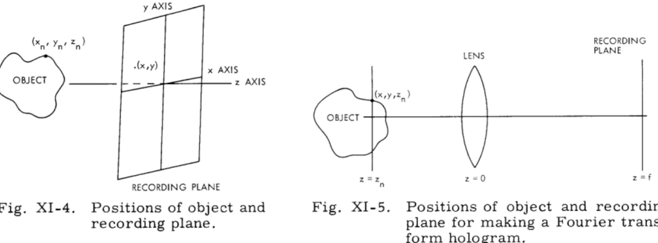
In the course of making a synthesized hologram of a three-dimensional object, we need a method to compute the wave front of the object on a particular recording plane. Thus far, the method of finding the wave front of an object has been based on the point radiator approach.5 That is, in finding the wave front of the object each point of the object is regarded as a point radiator. For a point located at (xn, Yn, z n) in space the wave front of the point can be approximated by

W(x, y; Xn, y, z) = S(x , Yn, Zn) exp jTr ((X-x)2(y-yn)2 )/z n]. (4) The position of the point and the recording plane for obtaining W(x, y; xn, n', zn) is

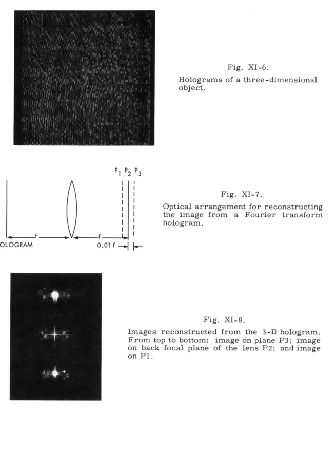
illus-trated in Fig. XI-4. The expression in Eq. 4 is the Fresnel approximation of a point source. If we sum up all waves of the points that constitute the object, we have the wave front needed to generate a synthesized hologram. If we want to make a synthesized Fou-rier transform of the object, however, the wavelets that make up the total wave front

y AXIS (X Yn' Zn) RECORDING LENS PLANE .(x,y) x AXIS OBJECT z AXIS z=z z=0 z=f RECORDING PLANE

Fig. XI-4. Positions of object and Fig. XI-5. Positions of object and recording

recording plane. plane for making a Fourier

trans-form hologram.

will be slightly different from the expression in Eq. 4. Suppose that in making the Fou-rier transform hologram the object is located on one side of a lens. The arrangement for recording the hologram is shown in Fig. XI-5. The wave front on the back focal plane of the lens produced by a point of the object is approximately equal to

V(u, v; x, y, z ) = S(x, y, zn exp jT((t-x)2 +(s-y)2)

/x

(t2+s2 )/f] A

exp[jn((t-u) 2+(s-v) 2)/xf] dtds = P(u, v; x, y, z n) S(x, y, z n )

exp jT(1-Zn/f) (u2 +v2) /f - j 2 (xu+yv) /\f] (5) In Eq. 5, f is the focal length of the lens, and the area of integration, A, depends on the size of the lens. If the object is small in comparison with the aperture of the lens, the function P(u, v; x, y, z_{n )} is approximately a constant. Equation 5 is the

Fresnel-Kirchhoff diffraction formula with the Fresnel approximation. When there are more

of the points on that plane is given by

R(u, v; zn) = exp j'(l-z /f)(u2+v2)/XfI

j

The summation in Eq. 6 is the discrete Fourier transform of the two-dimensional pat-tern formed by the points lying on the same plane. The total wave front of the object is then equal to

F (u, v)= R(u,v; z n). (7)

n

To show that the theoretical result derived for the wave front of the object is valid, we have performed a simple experiment. The three-dimensional object comprises two images located at two different planes. If we use the formula in Eq. 6 to find the wave front of the object, the wave front for this simple experiment is equal to

F(u, v) = R(u,v; z1) + R(u, v; z2). (8)

In the actual experiment the values of z1 and z2 are f and 0. 99f, respectively. If we substitute these values in Eq. 7, the equation becomes

F(u, v) = S(x, y; z1) exp(-jZnr(xu+yv)/Xf) + exp[jn(u2 +v2)/(100f)] xy

S S(x, y; z2) exp(j27r(ux+vy)/Xf), (9)

xy

where f is equal to 500 mm and the wavelength X is chosen to be 6328 A. The nonlinear phase term associated with one of the Fourier transforms in Eq. 9 is the same as the transmission of a thin lens having a focal length of 100f. In the reconstruction process the nonlinear phase function will combine with the reconstruction lens to give an effec-tive focal length of 0. 99f. This means that we shall have the two images in the recon-struction process. One is located on the back focal plane of the reconstruction lens, and the other is separated from the first image by a distance equal to 0. l0f.

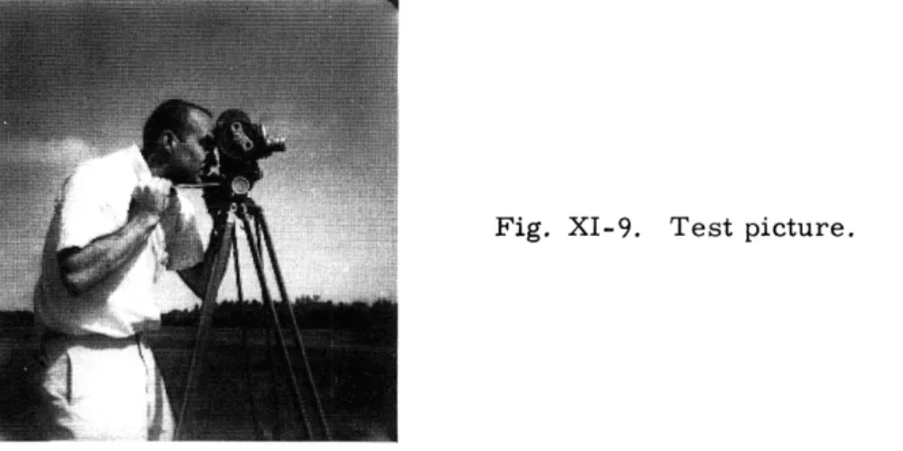
Figure XI-6 shows the hologram corresponding to the wave front in Eq. 9. Fig-ure XI-7 illustrates the arrangement used to reconstruct the images from the hologram and the three planes from which we can obtain sharp images. The images reconstructed from the hologram on the three planes are shown in Fig. XI-8. The letter 'E' has the Fourier transform, which is not modified by the nonlinear phase function. Therefore its image appears on the back focal plane of the lens. The symbol '+' has two images

object.

P1 P2 P3

HOLOGRAM 0.01 f .

K

Fig. XI-7.

Optical arrangement for reconstructing the image from a Fourier transform hologram.

Fig. XI-8.

Images reconstructed from the 3-D hologram. From top to bottom: image on plane P3; image on back focal plane of the lens P2; and image on P1.

in the reconstruction. They are the conjugate images of the symbol '+'.

The images reconstructed from the hologram have one interesting property. Because the technique that we use to record the depth information of the object is equivalent to

putting a small thin lens in contact with the Fourier transform of each of the layers of the object, the effective focal length of the reconstruction for the different layers is

dif-ferent. In using a lens and coherent light to obtain the inverse Fourier transform, the result is proportional to

f(x, y) = F(u,v) exp(j2(ux+vy)/Xf) dudv. (10)

-o -oo

Therefore the reconstructed image of the different layer will have a scale factor that is a function of the effective focal length. This property of the hologram can be observed in the reconstructed images of the symbol '+'. The image on plane P1 has an effective focal length shorter than the effective focal length of the image on plane P3. Hence the image on plane P1 is smaller than the image on plane P3. Generally, if we want to use the formula in Eq. 9, we must select a scale factor for the images in the different planes to compensate for the magnification in the reconstruction process.

W. H. Lee References

1. W-H. Lee, "Sampled Fraunhofer Hologram Generated by Computer," Quarterly

Progress Report No. 88, Research Laboratory of Electronics, M. I. T. , January 15, 1968, pp. 310-315.

2. System/360 Scientific Subroutine Package (360A-CM-03X) Version III Programmer's Manual. (276 p.)

3. H. J. Gerritsen, W. J. Hannen, and E. G. Ramberg, "Elimination of Speckle Noise with Redundancy," Appl. Opt. 7, 2301-2311 (1968).

4. G. B. Anderson and T. S. Huang, "Errors in Frequency Domain Processing of Image," Spring Joint Computer Conference, May 1969.

5. J. P. Waters, "Three-Dimensional Fourier-Transform Method for Synthesizing Binary Hologram," J. Opt. Soc. Am. 58, 1284 (1968).

B. PICTURE BANDWIDTH COMPRESSION USING FOURIER

ANALYSIS

1. Basic System Design a. Thresholding

Two main factors led to the bandwidth compression achieved by the scheme described in this report. The reduction in bits used for image representation is mainly due to

thresholding of coefficients in the frequency domain. Detection of areas of little impor-tance and subsequent simplified representation for these areas is also used in reducing

bandwidth.

The method of data compression begins by subdividing an image into square subsec-tions. The variance of each subsection is then measured to determine whether anything

significant occurs in the subsection. If the variance is less than a threshold value, the subsection is represented only by its average value and its variance. If the variance exceeds the threshold, the subsection is expanded in a two-dimensional Fourier series, and the Fourier coefficients are subjected to an adaptive thresholding procedure. The adaptive threshold for the Fourier coefficients is linearly proportional to the subsection variance. The energy of each coefficient is tested against the adaptive threshold. The number of coefficients passing the adaptive threshold test is compared with an integer

specifying the maximum allowable number of coefficients to be retained for transmis-sion. If the maximum allowable number of coefficients is exceeded, the adaptive thresh-old is raised and the Fourier coefficients are tested against the new threshthresh-old. The process is repeated until an allowable number of Fourier coefficients is obtained.

Image reconstruction from subsection data is simple. Subsections represented only by a variance and an average value parameter are filled in by statistically independent Gaussian random variables with variance and mean equal to the transmitted parameters. Fourier inversion is used in subsections having Fourier coefficient data.

b. Quantization and Coding

Linear adaptive quantization of the Fourier coefficients is performed with the max-imum Fourier coefficient, aside from the average value, determining the position of the largest quantization level for the magnitudes of the coefficients. The phases of the Fou-rier coefficients are linearly quantized on a scale from 0 to 2n. Partitioning of the

sub-sections represented by Fourier coefficients is based upon subsection variance. The subsections with the smaller variances are quantized with fewer levels than the higher energy subsections.

Data are needed to specify the positions in the frequency plane of the Fourier coef-ficients passing the adaptive energy threshold. Run-length coding is used, with the posi-tions of suprathreshold coefficients denoted by ones and other posiposi-tions denoted by zeros.

Each subsection of the image, including those with Fourier coefficient data, has quantized variance and average value parameters associated with it. A bit is also transmitted for each subsection to separate subsections without Fourier coefficient rep-resentation from those passing the variance test and having a Fourier coefficient representation. This additional bit permits the variance and average value parameters to be quantized with a differing number of levels for the two types of subsections.

2. Subjective Considerations a. Contrast Sensitivityl

The Weber fraction AB/B, which relates the just-noticeable difference in bright-ness AB to the background brightbright-ness B, is nearly constant for a wide range of values of B at approximately 2 per cent. This contrast sensitivity of the eye causes errors in images to tend to be more noticeable in the darker areas of images. If an image is to be subjected to an error environment, then the subjective quality of the resulting pic-ture normally improves if the effects of the error can be more evenly spread throughout the image, rather than being more pronounced in darker areas. Taking the logarithm of image brightness before processing and exponentiating after processing compensates for the eye's contrast sensitivity. This feature is incorporated in the design of our compression system.

b. Subsection Size

Choice of subsection size is influenced by different things. The larger subsection size is made, the more likely will areas of little energy be included with areas of large variance. This means that the total area of the picture represented by only average values and variances will decrease. Also, low-energy data, which need good reproduc-tion, are more likely to be lost, because of the presence of higher energy data in the

same subsection. This comes about because of the adaptive frequency-domain thresh-olding used in our compression scheme. Although it is not clear, it is also probably true that smaller subsection size results in more peaked Fourier spectra, because of

simplification in data structure. The smaller the subsection, the less likely will dif-ferent parts of the subsection cause frequency-domain averaging to result in a flattened

spectrum. The peaked spectrum can result in a representation by fewer Fourier coef-ficients than the flat spectrum. The subsection size cannot become too small, however, because the data-compression ratio will then be severely limited. Each subsection is represented by at least a mean value and a variance. The total number of these param-eters that is used to represent the entire image is inversely proportional to subsection

size.

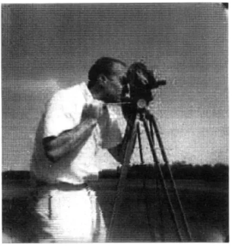
Subsection size was chosen to be 16 X 16 samples. This choice divided our 256 X 256 test picture into an integral number of subsections. It is interesting to note that when the picture appears at a distance from the eye of four times the picture height (normal viewing distance), the width of a subsection is roughly the period of the maximum spatial frequency response of the eye.

c. Variance Threshold

A grid was constructed on the test image of Fig. XI-9, partitioning the image into its subsections of size 16 X 16 samples. Variances were calculated for the logarithm

of brightness in each subsection. The image with superimposed grid was then viewed to determine which subsections appeared as random noise and could be represented by

Fig. XI-9. Test picture.

only a mean value and a variance. We found that a variance threshold could separate all subsections that looked like random noise from other subsections. There are 89 such subsections represented in Fig. XI-9.

d. Padding

Frequency-domain thresholding can cause very noticeable errors. Strong discon-tinuities often exist between brightness along an edge of a subsection and the opposite edge of the same subsection. The subsection is considered as a period of a periodic two-dimensional function when the subsection is expanded in a Fourier series. This periodic two-dimensional function has discontinuities corresponding to the discontinuities between opposite edges of the subsection. This causes interference in the frequency domain with spectra resulting from features within the subsection. Even worse, the error along a subsection edge in the reconstructed image tends to be correlated and, therefore, most displeasing. The edge error tends to be correlated because discon-tinuities between opposite edges in the original subsection tend to be correlated.

To eliminate the edge-to-edge discontinuity problem, "padding" of the subsection can be performed. Strips of additional samples can be added to two adjacent edges of the subsection before Fourier expansion. The samples in a strip will be interpolated from samples along the edge to which the strip is connected and samples along the opposite edge.

e. Frequency-Domain Quantization

Quantization of an image causes artifical contours to appear if too few quantiza-tion levels are used.2 Conventional television probably requires 6 or 7 bits of linear

brightness quantization for acceptable elimination of artificial contours. Random noise requires a higher energy to produce the same noticeability.3 Therefore, frequency-domain quantization, which acts to produce randomized noise in the image, should be more acceptable than brightness quantization of the same mean-square error. This will be true if one pitfall is avoided. The mean values of the subsections must be very finely quantized; otherwise, contours, which are easily detected by the eye, will appear along the boundaries of subsections in the reconstructed image. A bandwidth saving occurs with coarse quantizing of the other Fourier series coefficients.

f. Artificial Noise in Low -Variance Subsections

Random noise is generated in subsections of the reconstructed image, failing the variance threshold. If the noise in the input image is not too great, this should act to produce a more natural appearance in the system output. (Most areas of images have a granular or noisy appearance, because of a combination of texture in the original scene and film noise.) Also, the introduction of noise in these subsections tends to dis-guise defects that appear along subsection edges.

3. Experimental Results

The compression system described was simulated on the IBM 360/65 digital com-puter. A flying-spot scanner built by W. F. Schreiber served as an interface between the digital computer and picture hard copy.

Fig. XI-10. Output picture.

The picture in Fig. XI-10 is the result of the system acting on our test picture of Fig. XI-9. A total of 46, 632 bits was expended to "transmit" this image. This corre-sponds to a compression of 8. 43 to 1 in bandwidth when comparison is made with con-ventional 6-bit PCM

References

1. W. F. Schreiber, "Picture Coding," Proc. IEEE 55, 320-330 (1967).

2. T. S. Huang, O. J. Tretiak, B. Prasada, and Y. Yamaguchi, "Design Considerations in PCM Transmission of Low-resolution Monochrome Still Pictures," Proc. IEEE 55, 331-335 (1967).

3. L. G. Roberts, "Picture Coding Using Pseudorandom Noise," IRE Trans., Vol. IT-8, pp. 145-154, February 1962.

C. IMPULSE RESPONSE FOR A LENS WITH SEIDEL ABERRATIONS

For an optical system with axial symmetry, the retention of the first-order term in the series expansion of the angle characteristic leads to Gaussian optics. By including

the next higher order in the expansion, which includes five terms of the same order, the five Seidel aberrations may be treated. Each of these aberrations - spherical aberra-tions, coma, astigmatism, curvature of field, and distortion - arises because its cor-responding coefficient is nonzero.

For a lens satisfying Gaussian optics, a point source of light in the object plane produces a point source of light in the Gaussian image plane. Thus the impulse response, or point source response, of a system obeying Gaussian optics is again an impulse, but attenuated and displaced by the magnification factor. Let x denote object plane

coor--o

dinates, xi the image plane coordinates, and M the lateral magnification. Then an input

K(x)

brightness of 6(x o-x) will produce an output brightness of - 6(xi-Mx). The

func-IMI

tion K(x) accounts for the fraction of light intercepted by the lens and the transmission loss through the lens. To determine the image intensity distribution attributable to a surface in the object plane, besides knowledge of the impulse response of the lens, it is necessary to know the photometric nature of the object surface. For example, it may

radiate according to Lambert's law.

To account for aberrations in the lens, expressions for the ray aberration may be applied to find the impulse response. The ray aberration is a vector in the image plane from the Gaussian image point to the point where the actual ray intersects the image plane. For a Gaussian image point the ray aberration depends upon which ray from the object point is chosen.

Suppose the coordinate systems are as shown in Fig. XI-11. Let the following func-tions be given

x.i = Mx + Ax (u, v;x ,y_o)

The ray aberration is given by the vector (Ax, Ay). That is, the ray originating at object point (x o, ) and passing through exit pupil point (u, v) will deviate from the Gaussian

Yo V Y.

do AXIS OF

SYMMETRY

OBJECT EXIT IMAGE

PLANE PLANE PLANE

Fig. XI- 11. Coordinate system.

image point (Mx_{o ,} My_{o )} by (A , A y). In general, for a fixed object point several values of (u, v) may yield the same ray aberration. Let Be be the brightness (power/unit area)

at exit pupil point (u, v), and B. the brightness at the corresponding point (xi, yi). A small

II2

dv du

(u,v) (Xi ,Y) V

Fig. XI-12. Exit to image plane mapping.

rectangle in the exit pupil will be mapped into a small parallelogram in the image plane as shown in Fig. XI-12. Under the assumption that the power transferred down this ray tube is conserved, Be dudvI = B.iVIXVZ B. B dudv Bi= B_e V XV -1 -2 - a dv

-2

av

av

aAA_A y

u au

Bi = Be(u, v; x yo) det

00aA

y

x

av _v

= Be(u, v; x _, yo) (J(u, v; x_o, yo))- 1

Let n points in the exit pupil (u1,v l). .. . (un , v ) be mapped into the point (xi , Yi). Then the brightness at (x i , Yi) is

n

B.i(xi, Yi; Xo' Yo) = Be(u vj; xo, Yo)(J(uj, vj; x yo))- 1 (1) j=1

Now it is simply an application of the formula (1) to find the impulse response for the five aberrations. All the ray aberration formulas that follow have been taken from Born

and Wolf.1 Also, the object point will be at (0, yo), and polar coordinates (p, 0) in the exit pupil will be used to specify the ray aberration functions. The angle 0 is measured positive counterclockwise from the V-axis of Fig. XI-11. It will be assumed throughout that the optical system is simply a lens of radius RL.

1. Spherical Aberration

The ray aberrations for spherical aberration are

A = Bp_x 3 sin O

A = Bp cos 0

Y

and the Jacobian is

J(u, v; xo' Yo) = 3B2 p4.

Let (ro, 0 ) be polar coordinates of a unit point source in the object plane, and (ri', i) be polar coordinates measured from the Gaussian image point. Both 00 and

i should be measured from the x axes.

d

+p2

Be (p, 0;r, ) =o r2 +d +2pr sin (0 - 0

Also, r. = Bp3, and . = 0+ The variable d is the distance between the object plane

and the exit plane.

The output brightness distribution is

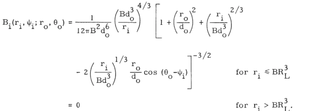
Bi(r111 _{i ,} i; ro , oo o )0 1 = 2 I2B2d6 4/3 Bd ri 3ri - -3/2 (6 -l ) for r. BR 3 1 L for r > BRL'

Regardless of the position of the point source in the object plane, a spot with nonuniform brightness of radius BR3 is the image. In general, the spot will have the same shape as

B.

0,

ro RL 1 do do 5

Fig. XI-13. Spherical aberration: Impulse response for an on-axis object. 2 /r \ +1 0 do 2/3 Bd3

1

do

,. =0

2T

2

ro 5 Rd 5

d. 5 d. 5

Fig. XI-14. Spherical aberration: Impulse response for an off-axis object.

the exit pupil aperture, and a brightness distribution dependent upon the object point position. Even though the general formula for the impulse response indicates that it is not object position invariant, Figs. XI-13 and XI-14 show, for "reasonably small"

r R

o L

values of -d and d , that the response is practically

o o 1 2nB2/3d2 r 4 / 3 B= 0 1 e

Lo,

The ray aberrations for coma are

Ax = -Fyo2 sin 26

LCr__

-A = -Fy p2(2+ cos 20).

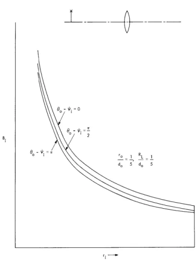
The boundary for the point (0, yo), 4 points

map into point.

impulse response is shown in Fig. XI-15. For a fixed object of the exit pupil map into each point in region I, and 2 points

Fig.

Fig. XI-15. Boundary of the coma pattern.

each point in region II. Let (x,y) be measured from the Gaussian image

x = x.

1

y = Yi - Myo"

The brightness distribution for x_{i ,}yi in region I is

Be (PI' _{1 ; 0, yo)} 2 2 P21 2 _- os 20

4F yop1 1-2cos 21111

For xi, Yi in region II the brightness distribution includes only the first two terms. The

variables pl, 11, 012' P2 21' 22 are functions of x, y as follows:

SF 0y( Y+ 2-3x2 S1 32 1 jl 2 2 j j = 1,2 QPR No. 93 Bi(x, y; 0, y ) = 248

2 2 j, 0 j.< -r

T < 4 - 2'r

The angles I ₁ and 2 are defined by Fig. XI-16. 3. Astigmatism and Curvature of Field

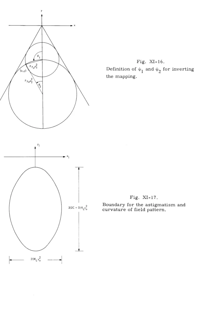
The ray aberrations in this case are 2

A

The elliptical boundary for the impulse response is shown in Fig. XI-17. Fortunately, this is a one-to-one mapping between the exit pupil and image plane, as was the mapping for spherical aberration. The brightness distribution is

B. (x, y; 0, yo) =

4 Be(p , 0; 0, yo),

ID(2C+D) Iyo

0,

The inversion of the mapping is

2 y 2 x2 24 2 4 4D y 4(2C+D) yo and 0 = 4, where sin = - x V/x +y y and cos = x +y

Besides the elliptical, instead of circular, boundary, this brightness distribution is sig-nificantly different from the one for spherical aberration because there is no singularity

in the brightness distribution at the Gaussian image point. 4. Distortion

The ray aberrations for distortion are A =0 x A = -Ey y o p -< RL p _RL

Definition of Il and 2 for inverting

the mapping.

2 2(2C + D) RLY

Fig. XI-17.

Boundary for the astigmatism and curvature of field pattern.

2

Since (Ax' Ay) are not functions of the exit pupil point, the brightness distribution is simply another impulse, but displaced.

G. M. Robbins References

1. M. Born and E. Wolf, Principles of Optics (Pergamon Press. London, 3rd edition,

1965).

D. SPECIFICATION OF THE PROSODIC FEATURES OF SPEECH

For several years, many research workers have been developing speech synthesis algorithms that operate directly on a string of phonemes representing the sound repre-sentation of the sentence under consideration. This phoneme sequence has usually been derived manually, but recently a scheme has been invented I to transform written words to their phonemic representation. Speech based on word-by-word phonemic representa-tion is usually intelligible, but not suitable for long-term use. Several problems remain, apart from those concerned directly with speech synthesis by rule from phonemic specifications.

First, many words can be nouns or verbs, depending on context [refuse, incline, survey], and proper stress cannot be specified until the intended syntactic form class is known. Second, punctuation and phrase boundaries may be used to specify pauses that help to make the complete sentence understandable. Third, more complicated

stress contours over phrases can be specified which facilitate sentence perception. Finally, intonation contours, or "tunes," are important for designating statements, questions, exclamations, and continuing or terminal juncture. These features (stress, intonation, and pauses) comprise the main prosodic or suprasegmental features of

speech.

Several experiments2 - 4 have shown that we tend to perceive sentences in chunks or phrasal units, and that the grammatical structure of these phrases is important for the correct perception of the sentence. It is also known 5 that the syntactic structure of the sentence is sufficient to specify much of the stress, pauses, and intonation of natural speech. Hence prosodic features of speech can be used in a limited fashion to help point out the intended surface syntactic structure of synthesized speech, which is then useful in the perception of the phonetic shape of the sentence.

It is desirable, then, to perform a limited parsing of sentences in order to allow the specification of the prosodic features of speech by rule. Such a scheme requires, first, the determination of the parts of speech of the words of the sentence; second, a phrase-level parsing of the sentence; and finally, execution of a phonological algorithm that

First, we consider determination of the parts of speech of words. The starting point for this procedure is the given word converted into one or more "morphs," each of which is either a prefix, base word, or suffix. Thus [grasshopper] - [grass] + [hop] + [er],

[browbeat] - [brow] + [beat], and [unfit] - [un] + [fit]. Each of these morphs corresponds to a dictionary entry that contains, in addition to phonemic specifications,

parts-of-speech information. In the case of base word morphs, this information consists of a set of parts of speech for that word, called the "grammatical homographs" of the word. For prefixes and suffixes, information is given indicating the resultant part of speech when the prefix or suffix is concatenated with a base word. Thus [-ness] always forms

a noun, as in [goodness].

Other researchers6, 7 have used a computational dictionary to compute parts of speech, relying on the prevalence of function words (determiners, prepositions, con-junctions, and auxiliaries), together with suffix rules of the type just described and their accompanying exception lists. This procedure, of course, keeps the lexicon small, but results in arbitrary parts-of-speech classification when the word is not a function word, and does not have a recognizable suffix. Furthermore, ambiguous suffixes such as

[-s]

(implying plural noun or singular verb) carry over their ambiguity to the entire word, whereas if the root word has a unique part of speech, like [cat], our procedure gives a unique result; [cats] (plural noun). Hence the morph lexicon can often be used to advan-tage, especially in the prevalent noun/verb ambiguities.

The parts-of-speech algorithm considers each morph of the word and its relation with its left neighbor, starting from the right end of the word. If there are two or more suffixes [commendables], they are entered into a last-in first-out pushdown list. Then the top suffix is joined to the root morph, and the additional suffixes are concatenated until the list is empty. Compounding is done next, and finally any prefixes are attached. Prefixes generally do not affect the part of speech of the base word, except for [em-, en-, be-] which imply verb as the resultant part of speech. Compounds can occur in English in any of three ways, and there appears to be no reliable method for dis-tinguishing these classes. There can be two separate words [bus stop], two words hyphenated [hand-cuff], or two words concatenated directly, as in [sandpaper]. The parts-of-speech algorithm treats the last two cases, leaving the two-word case for the parser to handle. The algorithm ignores the presence of a hyphen, and then processes hyphenated and one-word compounds as though they were both single words. The parts of speech of the two elements of the compound are considered as row and column entries to a matrix whose cells yield the resulting part of speech. Thus Adverb • Noun - Noun, as in [underworld]. _{Combinations of suffixes with compounds [handwriting] can be} accommodated, as well as one-word compounds containing more than two morphs.

A special routine is provided to handle troublesome suffixes such as [-er, -es, -s],

In this way, the algorithm makes use of the parts-of-speech information of the indi-vidual morphs to compute the parts-of-speech set for the word formed by these morphs. These sets then serve as input to the parser, after having first been ordered to suit the principles of the parser.

1. Parsing

Our goal is to determine the syntactic structure that is sufficient to specify the pro-sodic features of the sentence, which can then serve as cues to the perception of the intended text. Since we are trying to provide only a limited number of such cues (enough to allow the structure to be deduced), we have designed a limited parser that reveals the syntax of only a portion of the sentence. We have tried to find the simplest parser consistent with these phonological goals that would also use minimum core storage and run fast enough to allow for a realistic speaking rate, say, 150-180 words per minute. Because the absence, or incorrect implementation of prosodics in a small percentage of the output sentences is not likely to be catastrophic, we can tolerate occasional mis-takes by the parser, but we have tried to achieve 90 per cent accuracy. These require-ments, for a limited, phrase-level parser operating in real-time at comfortable speaking rates within restricted core storage, are indeed severe, and many features found in other parsers are absent here. We do not use a large number of parts-of-speech clas-sifications, nor do we exhaustively cycle through all the homographs of the words of a sentence to find all possible parsings. Inherent syntactic ambiguity ([They are washing machines]) is ignored, the resulting phrase structures being biased toward noun phrases and prepositional phrases. No deep-structure "trees" are obtained, since these are not needed in the phonological algorithm, and only noun phrases and prepositional phrases are detected, so that no sentencehood or clause-level tests are made. We do, however, compute a bracketed structure within each detected phrase, such as [the [old house]] and [in [[brightly lighted] windows]], since this structure is required by the phonolog-ical algorithm. The result is a context-sensitive parser that avoids time-consuming enumerative procedures, and consults alternative homographs only when some condition is detected (such as [to] used to introduce either an infinitive or a prepositional phrase) which requires such a search.

The parser makes two passes (left-to-right) over a given input sentence. The first pass computes a tentative bracketing of noun phrases and prepositional phrases. Inas-much as this initial bracketing makes no clause-level checks and does not directly exam-ine the frequently occurring noun/verb ambiguities, it is followed by a special routexam-ine designed to resolve these ambiguities by means of local context and grammatical number agreement tests. These last tests are also designed to resolve noun/verb ambiguities that do not occur in bracketed phrases, as [refuse] in [They refuse to leave]. As a result

of these two passes, a limited phrase bracketing of the sentence is obtained, and some ambiguous words have been assigned a unique part of speech, yet several words remain as unbracketed constituents.

The first pass is designed to quickly set up tentative noun phrase and prepositional phrase boundaries. This process may be thought of as operating in three parts. The program scans the sentence from left to right looking for potential phrase openers. For example, determiners, adjectives, participles, and nouns may introduce noun phrases, and prepositional phrases always start with a preposition. In the case of some intro-ducers, such as present participles, words further along in the sentence are examined, as well as previous words, to determine the grammatical function of the participle, as in [Wiring circuits is fun.]. Once a phrase opener has been found, very quick relational tests between neighboring words are made to determine whether the right phrase

bound-ary has been reached. These checks are possible because English relies heavily on word order in its structure. Having found a tentative right phrase boundary, right context

checks are made to determine whether or not this boundary should be accepted. After completion of these checks, the phrase is closed and a new phrase introducer is looked for. The procedure continues until the end of the sentence is reached.

When the bracketing is complete, further tests are made to check for errors in bracketing caused by frequent noun/verb ambiguities. For example, the sentence [That

old man lives in the gray house.] would be initially bracketed [That old man lives1

p [in the gray house]Pre_{p P.}

Notice that sentencehood tests (although not performed by the parser) would immediately reveal that the sentence lacks a verb, and further routines could deduce that [lives], which can be either a plural noun or a third person singular verb, is functioning as a verb, although the bracketing routine, since it is biased toward noun homographs, made

[lives] part of the noun phrase. We also note the importance of this error for the pho-netic shape of the sentence, since [lives] changes its phonemic structure according to its grammatic function in the sentence. An agreement test, however, compares the rightmost "noun" with any determiners that may reflect grammatical number. In this case, [that] is a singular demonstrative pronoun, so we know that [lives] does not agree with it, and hence must be a verb. After the agreement test has been made for each noun phrase, local context checks are used in an attempt to remove noun/verb ambigu-ities that are important for the phonological implementation, and yet have not been bracketed into phrases containing more than one word. Thus in the sentence [They produce and develop many different machines.], the algorithm would note that [produce] is immediately preceded by a personal pronoun in the nominative case, and hence the word is functioning as a verb. Such knowledge can then be used to put stress on the sec-ond syllable of the word in accordance with its function.

At the conclusion of the parsing process described above, phrase boundaries for noun phrases and prepositional phrases have been marked, but the structure within the phrase is not known. In order to apply the rules that are used for computing stress patterns within the phrase, however, internal bracketing must be provided. For this

rea-son, determiner-adjective-noun sequences are given a "progressive" bracketing, as [the[long[red barn]]], whereas noun phrases beginning with adverbials are given "regres-sive" bracketings, as [[[very brightly] projected] pictures]. A preposition beginning a prepositional phrase always has a progressive relation to the remaining noun phrase, so that we have [in [the [long [red barn]]]] and [ of [[[ very brightly] projected] pictures]].

Furthermore, two nouns together, as in [the local bus stop], are marked as a compound for use by the phonological algorithm.

The procedure described above is thus able to detect noun phrases and prepositional phrases and to compute the internal structure of these phrases. The grammar and parsing logic are intertwined in this procedure, so that an explicit statement of the grammar is difficult. Nevertheless, the rules are easily modified. At present, however, the provision of prosodics is supplied for noun phrases and prepositional phrases only.

2. Phonological Algorithm

Once noun phrases and prepositional phrases have been detected, the phonological algorithm uses the surface syntactic bracketing, plus punctuation and clause-marker words, to deduce the pattern for stress, pauses, and intonation related to the detected phrases.

Stress is implemented within the detected phrases by iterative use of the stress cycle rules, described by Chomsky and Halle. 5 These rules operate on the two constituents within the innermost brackets to specify where main stress should be placed. All other

stresses are then "pushed down" by one. (Here, "one" is the highest stress.) The inner-most brackets are then "erased," and the rules applied to the next pair of constituents.

The cycle is then continued until the phrase boundaries are reached. For compounds, the rules specify main stress on the leftmost element (compound rule), whereas for all

other syntactic units (e. g. , phrases) main stress goes on the rightmost unit (nuclear stress rule). For example, we have

[the [long[red barn]]] 2 1

4 2 3 1

where initially stress is 1 on all units except the article the, and two cycles of the phrase rule are used. The parser has, of course, provided the bracketing of the phrase. Also,

[ in [[[ very brightly] lighted] rooms]]

2 1

3 2 1

4 4 3 2 1

requires three applications of the rules, and [the [new [bus stop]]]

1 2

2 1 3

4 2 1 3

which contains a compound, requires two iterations. Each morph in the lexicon is given lexical stress, so that the phrase-level stress numbers described above provide the framework for the local stress variations of individual morphs or words.

Pauses are provided in a definite hierarchy throughout each sentence. Although we have not determined optimal values for these durations, pauses are used at phrase boundaries, where punctuation appears, and before clause-marker words such as [that, since, which]. _{Finally, terminal pauses are used between sentences. Much work} remains to be done on the acoustic correlates of juncture and stress, and several exper-iments are currently contributing to our understanding of these phenomena.

The provision of intonational fo contours by rule has been described by Mattingly,8 and our technique is similar to his. The slope of the f contour is controlled by the specific phonemes encountered in the sentence, and by the nature of the pause at the end of the phrasal unit. _{Rising terminal contours are specified at the end of} interroga-tive clauses just preceding the question mark, except when the clause starts with a [wh-] word, as [where is the station?]. _{In the absence of a question mark, the intonation} fo contour is falling with a slope determined by rules like those of Mattingly.

Work is continuing on improvements for the parser. We are focusing particularly on adverbial functions and the use of prepositions in verb phrases. We hope that sev-eral additional classes of phrases can be detected within the present parser framework. Also, the parsing scheme is being implemented to run in real time on a PDP-9

com-puter. We have developed a list structure to expedite this task, and the algorithms are being coded by using these low-level list handlers to provide maximum speed in minimum

core storage.

J. Allen References

1. _{F. F. Lee, "A Study of Grapheme to Phoneme Translation of English," Ph.D. Thesis,}

M. I.T. , 1965.

2. _{G. A. Miller, "Decision Units in the Perception of Speech," IRE Trans., Vol. IT-8,} No. 2, p. 81, February 1962.

3. G. A. Miller, G. A. Heise, and W. Lichten, "The Intelligibility of Speech as a Func-tion of the Context of the Test Materials," J. Exptl. Psychol. 41, 329 (1951).

4. G. A. Miller and S. Isard, "Some Perceptual Consequences of Linguistic Rules," J. Verb. Learn. and Verb. Behav. 2, 217 (1963).

5. N. Chomsky and M. Halle, Sound Patterns of English (Harper and Row Publishers, Inc., New York, 1968).

6. S. Klein and R. F. Simmons, "A Computational Approach to the Grammatical Coding of English Words," J. Acoust. Computing Machinery 10, 334 (1963).

7. D. C. Clarke and R. E. Wall, "An Economical Program for the Limited Parsing of English," AFIPS Conference Proceedings, 1965, FJCC, p. 307.

8. J. G. Mattingly, "Synthesis by Rule of Prosodic Features," Language & Speech 9, 1 (1966).

E. "OPTICAL BENCH" SIMULATOR

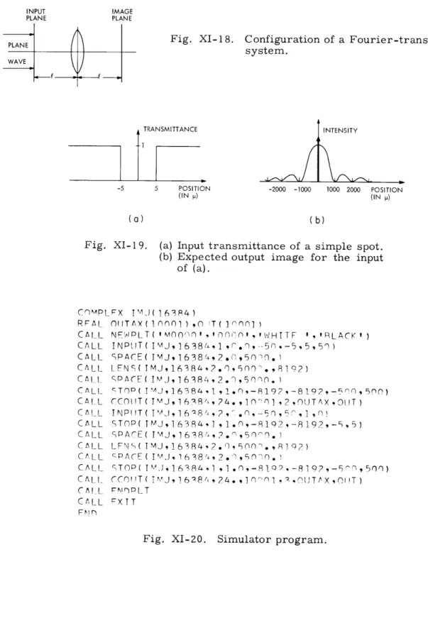
A program has been developed for the simulation of one-dimensional optical systems.

Analysis of an optical system is performed with the use of results derived by Vander Lugt1 and Goodman. 2 The approach is to characterize each element of an

opti-cal system, for example, lens or stop, by its impulse response, or equivalently, by its system function in the frequency domain. The light distribution may then be followed through the system and sequentially processed by each element.

A Fortran program has been written to accomplish the procedure outlined above. The equations were put in a discrete form, and a Fast Fourier Transform package was utilized. The sample spacing in the field was scaled to 1 l. Maximum field size is lim-ited only by available core memory. Test programs have been run on the M. I. T.

Com-putation Center's IBM System 360 with field lengths of a few centimeters.

The user's program consists in calls to various subroutines with appropriate argu-ments. Each subroutine corresponds to a basic element of the optical system, or to a certain output function. The available elements are briefly described as follows.

INPUT - sets up a monochromatic plane wave across the field.

STOP - places a stop in the optical path whose transmittance function can be square or sinusoidal over variable limits.

LENS - places a lens in the optical path whose radius and focal length are variable. SPACE - gives a desired separation to any of the elements above.

These elements may be cascaded indefinitely, and objects may be called consecu-tively to form compound elements. Two output routines, OUTPUT and CCOUT, which plot the light intensity as a function of position for any point on the axis, are available. OUTPUT plots the intensity on the computer print-out, while CCOUT utilizes the Cal Comp plotter. The subroutines are called in the order of their position on the

Fig. XI-18. Configuration of a Fourier-transforming system. TRANSMITTANCE -5 5 POSITION (IN p) (a) Fig. XI-19. COMPL CALL CALL CALL CA L L CA LL CA I_.-C LL ._ CALL CALL CA LL CA LL C ^LL INTENSITY -2000 -1000 1000 2000 POSITION (IN ) (b)

Input transmittance of a simple spot. Expected output image for the input of (a). FX IM J( 163 4) nrITAX (1n ( n ) ,O T( ] nn] ) N E. P L T ( M)O( ,) , n-r ,' H I T F 'RLACK R ) INPUT( SPACE( qPACE( STOD( I CCO T IT( I NP IT( STOP( I SPACE( LFNS( I aPACE( CTOD( I IMJ,1638t,1 , .q, -5 ,-5,,5q) IMJ 1638492*.0,( 50 ,0. MJ 16384,2.qr)5n '.,8192) !MJ,16384,2. ,5Sq . ) J 1.6384,l1 9 1J *r)-8192 -8192 - 0 ,500)

IMJ,1 6 8/ , 24. ,10l O -) 2~-, JTAX ,O)lT)

IMJ, 1 6 84 , 2 ,T .n,--59, r , rn)

M.J,]6384,1 1 on -,192,-8]192 - 5,5) I MJ 1 638~ 2 ,

M J,16384,2.2,°9 ,5R1

MJ,]6384, 1 .n - 19 ,-8]92 9) , -5 0~ CALI I C Cr)riIT ( iMJ ,1i6 8/ia2 4 ., 1 'I '1 * ? .CIJiT

~X

CAI _

C L_ L

FM 9

X IT

r.i. I I I I: I I i I I I I I: I I I: I 1t i . i

ii '

I- I

I/

Ii

xxr~lI

1

i ii I

Fig. XI-21. (a) Input intensity for square transmittance function.

(b) Input intensity for sinusoidal transmittance function.

A A AISIVAAAJ -~ ~ -T7~ -~25~ 350 050 9 COOROINATE (a 0 0 am 225MI 31 IN MICRONS

--6 - -7MN -MA -ism -35C 300 ' '2-0 1 225" 3'50 36& 40;

X C.:0INqTE IN MICRONS

(b)

Fig. XI-22. (a) Output image for square input transmittance function.

(b) Output image for sinusoidal input transmittance function.

axis or their desired execution. Plots may be called at any point without affecting the following operations.

One of the advantages of the system is the ease with which the experimenter can study the effects of details such as lens size on his desired image. The effects of stops at various positions and with various sizes can be easily judged by direct comparison of the output images. The following example demonstrates the use of the simulator for comparing the effects of two different types of stops.

Figure XI-18 shows the configuration of a Fourier-transforming optical system. The transform of the input field, appropriately scaled, appears at the back focal plane of the lens. We wish to identify the size of a small spot on the input plane from the observed Fourier transform image. The spot transmittance, for a 10-p spot, and its expected transform in the image plane, are shown in Fig. XI-19. We also wish to cut down on the incident light by placing the spot in an aperture of approximately 50 Lp. Two such apertures are considered. One has a square transmittance function, while the other has a gradual, sinusoidal transmittance. (The transmittances are shown in Fig. XI-21.) The simulation program for these configurations is shown in Fig. XI-20. The field width is 16, 384 points. It should be noted that INPUT has the capability of producing a stop after initialization. In fact, STOP is simply an entry to that part of INPUT. The calls to OUTPUT produce the intensity graphs shown in Fig. XI-21. These are plots of the input intensity and are plotted on the print-out sheet. Stops were introduced at the image plane which block the high intensity on the optic axis. Since the Cal Comp routines auto-matically scale the output graph, this blocking was necessary to expand the size of the tails of the image. The final images from the Cal Comp plotter are shown in Fig. XI-22. It can be seen that the sinusoidal aperture gives a much clearer image which would be more easily recognized as the transform of a 10-p spot.

Optical Bench is available from the Biological Image Processing section of C. I. P. G. J. E. Bowie References

1. A. Vander Lugt, "Operational Notation for the Analysis and Synthesis of Optical Data

Processing Systems," Proc. IEEE 54, 1055-1063 (1966).

2. J. Goodman, Introduction to Fourier Optics (McGraw-Hill Publishing Company, New York, 1968).

F. INITIAL STUDIES ON THE ACOUSTIC CORRELATES OF PROSODIC FEATURES FOR A READING MACHINE

1. Introduction

For several years, a reading machine has been under development in the Cognitive Information Processing Group of the Research Laboratory of Electronics. The final purpose of this machine is to take printed text as input and to give as output an intel-ligible spoken equivalent. To realize these aims, pattern recognition routines have been developed to gather the text information,l a grapheme-to-phoneme conversion routine

2

has been written to transform the text information into its phonemic equivalent, a lim-ited sentence parser has been produced to supply structural information,3 and phonemic

synthesis programs have been written to produce the output speech.4' 5

Some important problems remain to be solved before the reading machine can really become a viable system. Among these is the problem of correctly using the structural

information, made available by the parser, to control the acoustic correlates for the pro-sodic features (stress, juncture, and intonation) of the speech signal. This is important for two reasons. First, a great deal of information is available through the sentence structure, and needs to be transmitted to the listeners. Second, the correct generation of the acoustic correlates for the various prosodic features tends to make the speech more "natural." This, in turn, increases intelligibility and the "ease" with which a lis-tener can understand what is being spoken.

Since the parser for the reading machine is a phrase-level parser, the problem of the acoustic correlates of stress, intonation, and juncture is currently being approached on a phrase level. The acoustic correlates under study, at present, are fundamental frequency, duration (particularly vowel durations), intensity, and pauses. It is the pur-pose of this report to describe briefly the tact being used in studying these acoustic cor-relates of prosodic features as they apply to the reading machine, to discuss in some detail the results of one recent experiment, and to indicate the direction of other work in this area.

2. Problems of Describing the Acoustic Correlates of Prosodic Features in the Reading Machine Environment

Any work associated with the reading machine is subject to several constraints, because of the character and goals of the over-all project itself. One of these constraints

is, of course, that all processing must be done automatically, but this alone cannot make the reading machine a usable product. Another constraint is that any rules written for use with the reading machine must also conform to the "real time" goals of the project,

and, likewise, since many computer programs must be used in processing a sentence from recognition to speech, any written computer code must be as compact as possible.

Hence, the first thing that must be remembered in writing any rules for the reading machine is that they must function as well as possible and still not require an unreason-able amount of processing time or computer space.

In this context, then, the problem of describing the acoustic correlates for stress, intonation, and juncture can be restated as follows. Given as an input the phonemic

strings and word-level stress supplied by the grapheme-to-phoneme conversion routines, and given the phrase-level structure supplied by the parser, find a set of rules for con-trolling fundamental frequency, phoneme duration, phonemic intensity, pause durations,

and phonemic quality which are sufficient to transfer to a listener the available struc-tural information in a way that he perceives as nastruc-tural. Notice here that there is no

requirement to describe all of the acoustic phenomena associated with prosodic features in real speech. Clearly, the mapping from derived constituent structure to the acoustic correlates of prosodic feature in real speech is many to one, being effected by dialectic variation, the idiosyncrasies of individual subjects, and semantic and emotional consid-erations. What is sought, rather, are rules describing one such mapping that is accept-able from a perceptual viewpoint. There is hence no requirement that the rules reflect any fundamental truths about speech or speech production, but only that they give one legitimate set of output acoustic correlates as described above.

The approach now being used in solving this problem can be stated as follows. First, study the effects of various lexical (word) stress patterns on fundamental frequency, phoneme duration, etc. in words spoken in isolation (one-word phrases or sentences).

Then observe these words in various structural positions in phrases, and try to describe systematically the variations in the various acoustic correlates attributable to structure. In this way, we hope that a hierarchy of rules, working from the word level to the phrase level, may be devised.

Before going on to describe one of the initial experiments, a word on the collection of data is in order. First, it is a well-known fact that there are a great many individual differences between the speech produced by different subjects. Hence, if consistent results are desired, it is important to analyze the data from each subject individually, and then look for general patterns in the data. Second, it is also known that not all var-iations in the various acoustic correlates that are being studied are related to structure. For example, it is known that vowel duration is affected by the following consonant, and, likewise, phonemes in general vary in length because of their syllabic position. Hence, where the effects of structure alone are sought, it is desirable, whenever possible, to

describe the other known effects and "normalize" them out. Third, there is the problem of describing "phonemic duration" in a systematic way. A "phoneme" is, in fact, an

abstract linguistic entity, and does not inherently have a "duration." Hence, a set of rules for consistently placing phonemic boundaries were devised which were meaningful from the point of view of the speech synthesis routines. These rules, however, do not