HAL Id: hal-01148958
https://hal.archives-ouvertes.fr/hal-01148958
Submitted on 26 May 2015
HAL is a multi-disciplinary open access
archive for the deposit and dissemination of
sci-entific research documents, whether they are
pub-lished or not. The documents may come from
teaching and research institutions in France or
abroad, or from public or private research centers.
L’archive ouverte pluridisciplinaire HAL, est
destinée au dépôt et à la diffusion de documents
scientifiques de niveau recherche, publiés ou non,
émanant des établissements d’enseignement et de
recherche français ou étrangers, des laboratoires
publics ou privés.
New characterizations of minimum spanning trees and of
saliency maps based on quasi-flat zones
Jean Cousty, Laurent Najman, Yukiko Kenmochi, Silvio Guimarães
To cite this version:
Jean Cousty, Laurent Najman, Yukiko Kenmochi, Silvio Guimarães. New characterizations of
mini-mum spanning trees and of saliency maps based on quasi-flat zones. 12th International Symposium
on Mathematical Morphology (ISMM), Benediktsson, J.A.; Chanussot, J.; Najman, L.; Talbot„ May
2015, Reykjavik, Iceland. pp.205-216, �10.1007/978-3-319-18720-4_18�. �hal-01148958�
New characterizations of minimum spanning trees
and of saliency maps based on quasi-flat zones
?Jean Cousty1, Laurent Najman1, Yukiko Kenmochi1, Silvio Guimarães1,2
1
Université Paris-Est, LIGM, A3SI, ESIEE Paris, CNRS {j.cousty, l.najman, y.kenmochi, s.guimaraes}@esiee.fr,
2 PUC Minas - ICEI - DCC - VIPLAB
Abstract. We study three representations of hierarchies of partitions: dendrograms (direct representations), saliency maps, and minimum span-ning trees. We provide a new bijection between saliency maps and hier-archies based on quasi-flat zones as used in image processing and char-acterize saliency maps and minimum spanning trees as solutions to con-strained minimization problems where the constraint is quasi-flat zones preservation. In practice, these results form a toolkit for new hierarchical methods where one can choose the most convenient representation. They also invite us to process non-image data with morphological hierarchies.
Keywords: Hierarchy, saliency map, minimum spanning tree
1
Introduction
Many image segmentation methods look for a partition of the set of image pixels such that each region of the partition corresponds to an object of interest in the image. Hierarchical segmentation methods, instead of providing a unique partition, produce a sequence of nested partitions at different scales, enabling to describe an object of interest as a grouping of several objects of interest that appear at lower scales (see references in [14]). This article deals with a theory of hierarchical segmentation as used in image processing. More precisely, we investigate different representations of a hierarchy: by a dendrogram (direct set representation), by a saliency map (a characteristic function), and by a minimum spanning tree (a reduced domain of definition). Our contributions are threefold: 1. a new bijection theorem between hierarchies and saliency maps (Th. 1) that relies on the quasi-flat zones hierarchies and that is simpler and more general than previous bijection theorem for saliency maps; and
2. a new characterization of the saliency map of a given hierarchy as the mini-mum function for which the quasi-flat zones hierarchy is precisely the given hierarchy (Th. 2); and
3. a new characterization of the minimum spanning trees of a given edge-weighted graph as the minimum subgraphs (for inclusion) whose quasi-flat zones hierarchies are the same as the one of the given graph (Th. 3).
?
This work received funding from ANR (contract ANR-2010-BLAN-0205-03), CAPES/PVE (grant 064965/2014-01), and CAPES/COFECUB (grant 592/08).
The links established in this article between the maps that weight the edges of a graph G, the hierarchies on the vertex set V(G) of G, the saliency maps on the edge set E(G) of G, and the minimum spanning trees for the maps that weight the edges of G are summarized in the diagram of Fig. 1.
Q F Z
Saliency maps on E(G)
(P1):Φ−1=Q F Z Q F Z
Connected hierarchies on V (G)
Maps on E(G) Minimum spanning trees
⊆
(P2): constrained minimization for
Φ
(P3): constrained minimization for
Ψ
the inclusion relation ⊑ on graphs.
the ≤ ordering on maps.
Fig. 1. A diagram that summarizes the results of this article. The solutions to prob-lems (P1), (P2), and (P3) are given by Ths. 1, 2, and 3, respectively. The constraint
involved in (P2) and (P3) is to leave the induced quasi-flat zones hierarchy unchanged.
In the diagram, QF Z stands for quasi-flat zones (Eq. 3), and the symbols Φ and Ψ stand for the saliency map of a hierarchy (Eq. 5) and of a map respectively (Section 5).
One possible application of these results is the design of new algorithms for computing hierarchies. Indeed, our results allow one to use indifferently any of the three hierarchical representations. This can be useful when a given oper-ation is more efficiently performed with one representoper-ation than with the two others. Naturally, one could work directly on the hierarchy (or on its tree-based representation) and finally compute a saliency map for visualization purposes. For instance, in [8, 17], the authors efficiently handle directly the tree-based rep-resentation of the hierarchy. Conversely, thanks to Th. 1, one can work on a saliency map or, thanks to Th. 3, on the weights of a minimum spanning tree and explicitly computes the hierarchy in the end. In [5, 15], a resulting saliency map is computed before a possible extraction of the associated hierarchy of wa-tersheds. In [9], a basic transformation that consists of modifying one weight on a minimum spanning tree according to some criterion is considered. The cor-responding operation on the equivalent dendrogram is more difficult to design. When this basic operation is iterated on every edge of the minimum spanning tree, one transforms a given hierarchy into another one. An application of this technique to the observation scale of [7] has been developed in [9] (see Fig. 2).
Another interest of our work is to precise the link between hierarchical clas-sification [16] and hierarchical image segmentation. In particular, it suggests that hierarchical image segmentation methods can be used for classification (the converse being carried out for a long time). Indeed, our work is deeply related to hierarchical classification, more precisely, to ultrametric distances, subdomi-nant ultrametrics and single linkage clusterings. In classification, representation
of hierarchies, on which no connectivity hypothesis is made, are studied since the 60’s (see references in [16]). The framework presented in this article deals with connected hierarchies and a graph needs to be specified for defining the connectivity of the regions of the partitions in the hierarchies. The connectivity of regions is the main difference between what has been done in classification and in segmentation. Rather than restricting the work done for classification, the framework studied in this article generalizes it. Indeed the usual notions of classification are recovered from the definitions of this article when a complete graph (every two points are linked by an edge) is considered. For instance, when a complete graph is considered, a saliency map becomes an ultrametric distance, which is known to be equivalent to a hierarchy. However, Th. 1 shows that, when the graph is not complete, we do not need a value for each pair of elements in order to characterize a hierarchy (as done with an ultrametric distance) but one value for each edge of the graph is enough (with a saliency map). Furthermore, when a complete graph is considered, the hierarchy of quasi-flat zones becomes the one of single linkage clustering. Hence, Th. 3 allows to recover and to gener-alize a well-known relation between the minimum spanning trees of the complete graph and single linkage clusterings.
(a) (b) (c) (d)
Fig. 2. Top row: some images from the Berkeley database [1]. Middle row: saliency maps according to [9] developed thanks to the framework of this article. Bottom row: segmentations extracted from the hierarchies with (a) 3, (b) 18, (c) 6 and (d) 16 regions.
2
Connected hierarchies of partitions
A partition of a finite set V is a set P of nonempty disjoint subsets of V whose union is V (i.e., ∀X, Y ∈ P, X ∩ Y = ∅ if X 6= Y and ∪{X ∈ P} = V ).
Any element of a partition P of V is called a region of P. If x is an element of V , there is a unique region of P that contains x; this unique region is denoted by[P]x. Given two partitions P and P0of a set V , we say that P0 is a refinement
of P if any region of P0 is included in a region of P. A hierarchy (on V ) is a sequence H = (P0, . . . , P`) of indexed partitions of V such that Pi−1 is a
refinement of Pi, for any i∈ {1, . . . , `}. If H = (P0, . . . , P`) is a hierarchy, the
integer ` is called the depth ofH. A hierarchy H = (P0, . . . , P`) is called complete
if P`={V } and if P0 contains every singleton of V (i.e., P0={{x} | x ∈ V }).
The hierarchies considered in this article are complete.
P1 P2 P3
P0
P0 P1 P2 P3 H
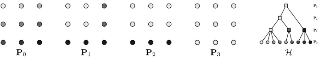
Fig. 3. Illustration of a hierarchy H = (P0, P1, P2, P3). For every partition, each
re-gion is represented by a gray level: two dots with the same gray level belong to the same region. The last subfigure represents the hierarchy H as a tree, often called a den-drogram, where the inclusion relation between the regions of the successive partitions is represented by line segments.
Figure 3 graphically represents a hierarchyH = (P0, P1, P2, P3) on a
rect-angular subset V of Z2made of 9 dots. For instance, it can be seen that P 1 is a
refinement of P2 since any region of P1is included in a region of P2. It can also
be seen that the hierarchy is complete since P0 is made of singletons and P3 is
made of a single region that contains all elements.
In this article, we consider connected regions, the connectivity being given by a graph. Therefore, we remind basic graph definitions before introducing connected partitions and hierarchies.
A (undirected) graph is a pair G = (V, E), where V is a finite set and E is composed of unordered pairs of distinct elements in V , i.e., E is a subset of{{x, y} ⊆ V | x 6= y}. Each element of V is called a vertex or a point (of G), and each element of E is called an edge (of G). A subgraph of G is a graph G0 = (V0, E0) such that V0 is a subset of V , and E0 is a subset of E. If G0 is
a subgraph of G, we write G0 v G. The vertex and edge sets of a graph X are
denoted by V(X) and E(X) respectively.
Let G be a graph and let (x0, . . . , xk) be a sequence of vertices of G. The
sequence (x0, . . . , xk) is a path (in G) from x0 to xk if, for any i in {1, . . . , k},
{xi−1, xi} is an edge of G. The graph G is connected if, for any two vertices x
and y of G, there exists a path from x to y. Let X be a subset of V(G). The graph induced by X (in G) is the graph whose vertex set is X and whose edge set contains any edge of G which is made of two elements in X. If the graph induced by X is connected, we also say, for simplicity, that X is connected (for G) . The
subset X of V(G) is a connected component of G if it is connected for G and maximal for this property, i.e., for any subset Y of V(G), if Y is a connected superset of X, then we have Y = X. In the following, we denote by C(G) the set of all connected components of G. It is well-known that this set C(G) of all connected components of G is a partition of V(G). This partition is called the (connected components) partition induced by G. Thus, the set[C(G)]xis the
unique connected component of G that contains x.
Given a graph G = (V, E), a partition of V is connected (for G) if any of its regions is connected and a hierarchy on V is connected (for G) if any of its partitions is connected.
For instance, the partitions presented in Fig. 3 are connected for the graph given in Fig. 4(a). Therefore, the hierarchyH made of these partitions, which is depicted as a dendrogram in Fig. 3 (rightmost subfigure), is also connected for the graph of Fig. 4(a).
For image analysis applications, the graph G can be obtained as a pixel or a region adjacency graph: the vertex set of G is either the domain of the image to be processed or the set of regions of an initial partition of the image domain. In the latter case, the regions can in particular be “superpixels”. In both cases, two typical settings for the edge set of G can be considered: (1) the edges of G are obtained from an adjacency relation between the image pixels, such as the well known 4- or 8-adjacency relations; and (2) the edges of G are obtained by considering, for each vertex x of G, the nearest neighbors of x for a distance in a (continuous) features space onto which the vertices of G are mapped.
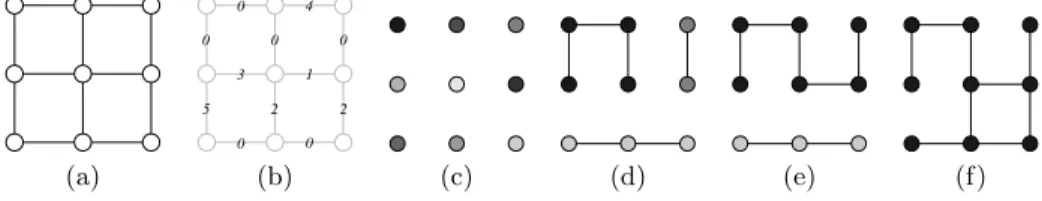
0 0 0 4 0 3 0 5 0 2 2 1 (a) (b) (c) (d) (e) (f)
Fig. 4. Illustration of quasi-flat zones hierarchy. (a) A graph G; (b) a map w (numbers in black) that weights the edges of G (in gray); (c, d, e, f) the λ-subgraphs of G, with λ = 0, 1, 2, 3. The associated connected component partitions that form the hierarchy of quasi-flat zones of G for w is depicted in Fig. 3.
3
Hierarchies of quasi-flat zones
As established in the next sections, a connected hierarchy can be equivalently treated by means of an edge-weighted graph. We first recall in this section that the level-sets of any edge-weighted graph induce a hierarchy of quasi-flat zones. This hierarchy is widely used in image processing [12].
Let G be a graph, if w is a map from the edge set of G to the set R+ of
positive real numbers, then the pair (G, w) is called an (edge-)weighted graph. If(G, w) is an edge-weighted graph, for any edge u of G, the value w(u) is called the weight of u (for w).
Important notation. In the sequel of this paper, we consider a weighted graph(G, w). To shorten the notations, the vertex and edge sets of G are denoted by V and E respectively instead of V(G) and E(G). Furthermore, we assume that the vertex set of G is connected. Without loss of generality, we also assume that the range of w is the set E of all integers from 0 to|E| − 1 (otherwise, one could always consider an increasing one-to-one mapping from the set {w(u) | u ∈ E} into E). We also denote by E• the set E∪ {|E|}.
Let X be a subgraph of G and let λ be an integer in E•. The λ-level set of X (for w) is the set wλ(X) of all edges of X whose weight is less than λ:
wλ(X) ={u ∈ E(X) | w(u) < λ}. (1)
The λ-level graph of X is the subgraph wV
λ(X) of X whose edge set is the λ-level
set of X and whose vertex set is the one of X:
wλV(X) = (V (X), wλ(X)). (2)
The connected component partition C(wV
λ(X)) induced by the λ-level graph
of X is called the λ-level partition of X (for w).
For instance, let us consider the graph G depicted in Fig. 4(a) and the map w shown in Fig. 4(b). The0-, 1-, 2- and 3-level sets of G contain the edges depicted in Figs. 4(c), (d), (e), and (f), respectively. The graphs depicted in these figures are the associated0-, 1-, and 3-level graphs of G and the associated 0-, 1-, 2-and3-level partitions are shown in Fig. 3.
Let X be a subgraph of G. If λ1and λ2are two elements in E•such that λ1≤
λ2, it can be seen that any edge of the λ1-level graph of X is also an edge of
the λ2-level graph of X. Thus, if two points are connected for the λ1-level graph
of X, then they are also connected for the λ2-level graph of X. Therefore, any
connected component of the λ1-level graph of X is included in a connected
component of the λ2-level graph of X. In other words, the λ1-level partition
of X is a refinement of the λ2-level partition of X. Hence, the sequence
QFZ(X, w) = (C(wV
λ(X))| λ ∈ E
•) (3)
of all λ-level partitions of X is a hierarchy. This hierarchyQFZ(X, w) is called the quasi-flat zones hierarchy of X (for w). It can be seen that this hierarchy is complete whenever X is connected.
For instance, the quasi-flat zones hierarchy of the graph G (Fig. 4(a)) for the map w (Fig. 4(b)) is the hierarchy of Fig. 3.
For image analysis applications, we often consider that the weight of an edge u={x, y} represents the dissimilarity of x and y. For instance, in the case where the vertices of G are the pixels of a grayscale image, the weight w(u) can be the absolute difference of intensity between x and y. The setting of the graph (G, w) depends on the application context.
4
Correspondence between hierarchies and saliency maps
In the previous section, we have seen that any edge-weighted graph induces a connected hierarchy of partitions (called the quasi-flat zones hierarchy). In this section, we tackle the inverse problem:
(P1) given a connected hierarchy H, find a map w from E to E such that the
quasi-flat zones hierarchy for w is preciselyH.
We start this section by defining the saliency map ofH. Then, we provide a one-to-one correspondence (also known as a bijection) between saliency maps and hierarchies. This correspondence is given by the hierarchy of quasi flat-zones. Finally, we deduce that the saliency map ofH is a solution to problem (P1).
Until now, we handled the regions of a partition. Let us now study their “dual” that represents “borders” between regions and that are called graph-cuts or simply cuts. The notion of a cut will then be used to define the saliency maps. Let P be a partition of V , the cut of P (for G), denoted by φ(P), is the set of edges of G whose two vertices belong to different regions of P:
φ(P) ={{x, y} ∈ E | [P]x6= [P]y} . (4)
Let H = (P0, . . . , P`) be a hierarchy on V . The saliency map of H is the
map Φ(H) from E to {0, . . . , `} such that the weight of u for Φ(H) is the maxi-mum value λ such that u belongs to the cut of Pλ:
Φ(H) (u) = max {λ ∈ {0, . . . , `} | u ∈ φ (Pλ)} . (5)
In fact, the weight of the edge u={x, y} for Φ(H) is directly related to the lowest index of a partition in the hierarchyH for which x and y belong to the same region:
Φ(H) (u) = minnλ∈ {1, . . . , `} | [Pλ]x= [Pλ]y
o
− 1. (6) For instance, if we consider the graph G represented by the gray dots and line segments in Fig. 5(a), the saliency map of the hierarchyH shown in Fig. 3 is the map shown with black numbers in Fig. 5(a). When the 4-adjacency relation is used, a saliency map can be displayed as an image (Figs. 5(e,f) and Fig. 2) which is useful for visualizing the associated hierarchy at a glance.
We say that a map w from E to E is a saliency map if there exists a hierar-chyH such that w is the saliency map of H (i.e. w = Φ(H)).
If ϕ is a map from a set S1 to a set S2 and if ϕ−1 is a map from S2 to S1
such that the composition of ϕ−1 with ϕ is the identity, then we say that ϕ−1 is the inverse of ϕ.
The next theorem identifies the inverse of the map Φ and asserts that there is a bijection between the saliency maps and the connected hierarchies on V . Theorem 1 The map Φ is a one-to-one correspondence between the connected hierarchies on V of depth |E| and the saliency maps (of range E). The in-verse Φ−1 of Φ associates to any saliency map w its quasi-flat zones hierarchy: Φ−1(w) =QFZ(G, w).
0 0 0 0 0 0 2 2 1 2 1 0 0 0 0 0 1 0 0 0 0 0 0 1 0 0 0 0 0 0 1 0 0 0 0 0 0 1 0 0 2 2 2 2 2 2 2 0 0 0 0 0 0 0 0 0 0 0 0 0 0 0 0 0 0 1 0 0 0 0 0 0 1 0 0 0 0 0 0 1 0 0 0 0 0 0 1 0 0 2 2 2 2 2 2 2 0 0 0 0 0 0 0 0 0 0 0 0 0 0 (a) (b) (c) (d) (e) (f)
Fig. 5. Illustration of a saliency map. The map (depicted by black numbers) is the saliency map s = Φ(H) of the hierarchy H shown in Fig. 3 when we consider the graph G depicted in gray. (b, c, d) the 1-, 2-, and 3-level graphs of G for s. The vertices are colored according to the associated 1-, 2-, and 3-level partitions of G: in each subfigure, two vertices belonging to a same connected components have the same grey level. Subfigures (e) and (f) show possible image representations of a saliency map when one considers the 4-adjacency graph.
Hence, as a consequence of this theorem, we haveQFZ(G, Φ(H)) = H, which means that H is precisely the hierarchy of quasi-flat zones of G for its saliency map Φ(H). In other words, the saliency map of H is a solution to problem (P1).
For instance, if we consider the hierarchyH shown in Fig. 3, it can be observed that the quasi-flat zones hierarchy for Φ(H) (see Fig. 5) is indeed H. We also deduce that, for any saliency map w, the relation Φ(QFZ(G, w)) = w holds true. In other words, a given saliency map w is precisely the saliency map of its quasi-flat zones hierarchy.
From this last relation, we can deduce that there are some maps that weight the edges of G and that are not saliency maps. Indeed, in general, a map is not equal to the saliency map of its quasi-flat zones hierarchy. For instance, the map w in Fig. 4 is not equal to the saliency map of its quasi-flat zones hierarchy which is depicted in Fig. 5. Thus, the map w is not a saliency map. The next section studies a characterization of saliency maps.
5
Characterization of saliency maps
Following the conclusion of the previous section, we now consider the problem: (P2) given a hierarchyH, find the minimal map w such that the quasi-flat zones
hierarchy for w is precisely H.
The next theorem establishes that the saliency map ofH is the unique solution to problem (P2).
Before stating Th. 2, let us recall that, given two maps w and w0 from E to E, the map w0 is less than w if we have w0(u)≤ w(u) for any u ∈ E.
Theorem 2 Let H be a hierarchy and let w be a map from E to E. The map w is the saliency map ofH if and only if the two following statements hold true:
2. the map w is minimal for statement 1, i.e., for any map w0 such that w0≤ w, if the quasi-flat zones hierarchy for w0 isH, then we have w = w0.
Given a weighted graph(G, w), it is sometimes interesting to consider the saliency map of its quasi-flat zones hierarchy. This saliency map is simply called the saliency map of w and is denoted by Ψ(w). From Th. 2, the operator Ψ which associates to any map w the saliency map Φ(QFZ(G, w)) of its quasi-flat zones hierarchy, is idempotent (i.e. Ψ(Ψ (w)) = Ψ (w)). Furthermore, it is easy to see that Ψ is also anti-extensive (we have Ψ(w)≤ w) and increasing (for any two maps w and w0, if w ≥ w0, then we have Ψ(w) ≥ Ψ(w0)). Thus, Ψ is a
morphological opening. This operator is studied, in different frameworks, under several names (see [11, 13, 10, 18, 16]). When the considered graph G is complete, it is known in classification (see, e.g., [16]) that this operator is linked to the minimum spanning tree of(G, w). The next section proposes a generalization of this link.
6
Minimum spanning trees
Two distinct maps that weight the edges of the same graph (see, e.g., the maps of Figs. 4(b) and 5(a)) can induce the same hierarchy of quasi-flat zones. Therefore, in this case, one can guess that some of the edge weights do not convey any useful information with respect to the associated quasi-flat zones hierarchy. More generally, in order to represent a hierarchy by a simple (i.e., easy to handle) edge-weighted graph with a low level of redundancy, it is interesting to consider the following problem:
(P3) given an edge-weighted graph (G, w), find a minimal subgraph X v G
such that the quasi-flat zones hierarchies of G and of X are the same. The main result of this section, namely Th. 3, provides the set of all solutions to problem (P3): the minimum spanning trees of (G, w). The minimum spanning
tree problem is one of the most typical and well-known problems of combinatorial optimization (see [3]) and Th. 3 provides, as far as we know, a new character-ization of minimum spanning trees based on the quasi-flat zones hierarchies as used in image processing.
Let X be a subgraph of G. The weight of X with respect to w, denoted by w(X), is the sum of the weights of all the edges in E(X): w(X) =P
u∈E(X)w(u).
The subgraph X is a minimum spanning tree (MST) of(G, w) if: 1. X is connected; and
2. V(X) = V ; and
3. the weight of X is less than or equal to the weight of any graph Y satisfying (1) and (2) (i.e., Y is a connected subgraph of G whose vertex set is V ). For instance, a MST of the graph shown in Fig. 4(b) is presented in Fig. 6(a). Theorem 3 A subgraph X of G is a MST of (G, w) if and only if the two following statements hold true:
1. the quasi-flat zones hierarchies of X and of G are the same; and
2. the graph X is minimal for statement 1, i.e., for any subgraph Y of X, if the quasi-flat zones hierarchy of Y for w is the one of G for w, then we have Y = X.
Theorem 3 (statement 1) indicates that the quasi-flat zones hierarchy of a graph and of its MSTs are identical. Note that statement 1 appeared in [6] but Th. 3 completes the result of [6]. Indeed, Th. 3 indicates that there is no proper subgraph of a MST that induces the same quasi-flat zones hierarchy as the initial weighted graph. Thus, a MST of the initial graph is a solution to problem (P3), providing a minimal graph representation of the quasi-flat zones
hierarchy of(G, w), or more generally by Th. 1 of any connected hierarchy. More remarkably, the converse is also true: a minimal representation of a hierarchy in the sense of(P3) is necessarily a MST of the original graph. To the best of our
knowledge, this result has not been stated before.
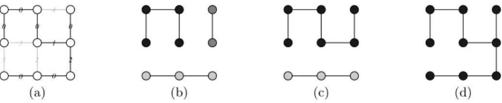
For instance, the level sets, level graphs and level partitions of the MST X (Fig. 6(a)) of the weighted graph(G, w) (Fig. 4) are depicted in Figs. 6(b), (c), (d). It can be observed that the level partitions of X are indeed the same as those of G. Thus the quasi-flat zones hierarchies of X and G are the same.
0 0 0 0 0 0 2 1 3 4 2 5 (a) (b) (c) (d)
Fig. 6. Illustration of a minimum spanning tree and of its quasi-flat zones hierarchy. (a) A minimum spanning tree X (black edges and black circled vertices) of the weighted graph of Fig. 4(b); (b, c, d) the 1- , 2-, and 3-level graphs of X. The vertices are colored according to the associated 1-, 2-, and 3-level partitions of X: in each subfigure, two vertices belonging to the same connected components have the same color.
7
Saliency map algorithms
When a hierarchyH is stored as a tree data structure (such as e.g. the dendro-gram of Fig. 3), the weight of any edge for the saliency map of this hierarchy can be computed in constant time, provided a linear time preprocessing. Indeed, the weight of an edge linking x and y is associated (see Eq. 6) to the lowest index of a partition for which x and y belongs to the same region. This index can be obtained by finding the index of the least common ancestor of{x} and {y} in the tree. The algorithm proposed in [2] performs this task in constant time, provided
a linear time preprocessing of the tree. Therefore, computing the saliency map ofH can be done in linear O(|E| + |V |) time complexity.
Thus, the complete process that computes the saliency map Ψ(w) of a given map w proceeds in two steps:
i) build the quasi-flat zones hierarchyH = QFZ(G, w) of G for w; and ii) compute the saliency map Ψ(w) = Φ(H).
On the basis of [6], step i) can be performed with the quasi-linear time algorithm shown in [15] and step ii) can be performed in linear-time as proposed in the previous paragraph. Thus, the overall time complexity of this algorithm is quasi-linear with respect to the size|E| + |V | of the graph G.
The algorithm sketched in [13], based on [4], for computing the saliency map of a given map w has the same complexity as the algorithm proposed above. However, the algorithm of [13] is more complicated since it requires to compute the topological watershed of the map. This involves a component tree (a data structure which is more complicated than the quasi-flat zones hierarchy in the sense of [6]), a structure for computing least common ancestors, and a hierarchical queue [4], which is not needed by the above algorithm. Hence, as far as we know, the algorithm presented in this section is the simplest algorithm for computing a saliency map. It is also the most efficient both from memory and execution-time points of view. An implementation in C of this algorithm is available at http://www.esiee.fr/˜info/sm.
8
Conclusions
In this article we study three representations for a hierarchy of partitions. We show a new bijection between hierarchies and saliency maps and we characterize the saliency map of a hierarchy and the minimum spanning trees of a graph as minimal elements preserving quasi-flat zones. In practice, these results allow us to indifferently handle a hierarchy by a dendrogram (the direct tree structure given by the hierarchy), by a saliency map, or by an edge-weighted tree. These representations form a toolkit for the design of hierarchical (segmentation) meth-ods where one can choose the most convenient representation or the one that leads to the most efficient implementation for a given particular operation. The results of this paper were used in [9] to provide a framework for hierarchicalizing a certain class of non-hierarchical methods. We study in particular a hierarchi-calization of [7]. The first results are encouraging and a short term perspective is the precise practical evaluation of the gain of the hierarchical method with respect to its non-hierarchical counterpart.
Another important aspect of the present work is to underline and to precise the close link that exists between classification and hierarchical image segmen-tation. Whereas classification methods were used as image segmentation tools for a long time, our results incite us to look if some hierarchies initially designed for image segmentation can improve the processing of non-image data such as data coming from geography, social network, etc.. This topic will be a subject of future research.
References
1. Arbelaez, P., Maire, M., Fowlkes, C., Malik, J.: Contour detection and hierarchical image segmentation. PAMI 33(5), 898–916 (2011)
2. Bender, M., Farach-Colton, M.: The LCA problem revisited. In: Latin American Theoretical INformatics. pp. 88–94 (2000)
3. Cormen, T.H., Leiserson, C.E., Rivest, R.L., Stein, C., et al.: Introduction to al-gorithms, vol. 2. MIT press Cambridge (2001)
4. Couprie, M., Najman, L., Bertrand, G.: Quasi-linear algorithms for the topological watershed. JMIV 22(2-3), 231–249 (2005)
5. Cousty, J., Najman, L.: Incremental algorithm for hierarchical minimum spanning forests and saliency of watershed cuts. In: ISMM. LNCS, vol. 6671, pp. 272–283 (2011)
6. Cousty, J., Najman, L., Perret, B.: Constructive links between some morphological hierarchies on edge-weighted graphs. In: ISMM, pp. 86–97. Springer (2013) 7. Felzenszwalb, P., Huttenlocher, D.: Efficient graph-based image segmentation.
IJCV 59, 167–181 (2004)
8. Guigues, L., Cocquerez, J.P., Men, H.L.: Scale-sets image analysis. IJCV 68(3), 289–317 (2006)
9. Guimarães, S.J.F., Cousty, J., Kenmochi, Y., Najman, L.: A hierarchical image segmentation algorithm based on an observation scale. In: SSPR/SPR, pp. 116– 125. Springer (2012)
10. Kiran, B., Serra, J.: Scale space operators on hierarchies of segmentations. In: Scale Space and Variational Methods in Computer Vision, vol. 7893, pp. 331–342 (2013) 11. Leclerc, B.: Description combinatoire des ultramétriques. Mathématiques et
Sci-ences humaines 73, 5–37 (1981)
12. Meyer, F., Maragos, P.: Morphological scale-space representation with levelings. In: Scale-Space Theories in Computer Vision, LNCS, vol. 1682, pp. 187–198 (1999) 13. Najman, L.: On the equivalence between hierarchical segmentations and
ultramet-ric watersheds. JMIV 40(3), 231–247 (2011)
14. Najman, L., Cousty, J.: A graph-based mathematical morphology reader. PRL 47(1), 3–17 (2014)
15. Najman, L., Cousty, J., Perret, B.: Playing with kruskal: algorithms for morpho-logical trees in edge-weighted graphs. In: ISMM, pp. 135–146. Springer (2013) 16. Nakache, J.P., Confais, J.: Approche pragmatique de la classification: arbres
hiérar-chiques, partitionnements. Editions Technip (2004)
17. Ravi Kiran, B., Serra, J.: Global–local optimizations by hierarchical cuts and climb-ing energies. PR 47(1), 12–24 (2014)
18. Ronse, C.: Ordering partial partitions for image segmentation and filtering: Merg-ing, creating and inflating blocks. JMIV 49(1), 202–233 (2014)

![Fig. 2. Top row: some images from the Berkeley database [1]. Middle row: saliency maps according to [9] developed thanks to the framework of this article](https://thumb-eu.123doks.com/thumbv2/123doknet/14331952.498310/4.918.210.716.525.801/berkeley-database-middle-saliency-according-developed-framework-article.webp)