HAL Id: hal-01245111
https://hal.archives-ouvertes.fr/hal-01245111
Submitted on 16 Dec 2015
HAL is a multi-disciplinary open access
archive for the deposit and dissemination of
sci-entific research documents, whether they are
pub-lished or not. The documents may come from
teaching and research institutions in France or
abroad, or from public or private research centers.
L’archive ouverte pluridisciplinaire HAL, est
destinée au dépôt et à la diffusion de documents
scientifiques de niveau recherche, publiés ou non,
émanant des établissements d’enseignement et de
recherche français ou étrangers, des laboratoires
publics ou privés.
Tensor Decomposition Exploiting Structural Constraints
for Brain Source Imaging
Hanna Becker, Ahmad Karfoul, Laurent Albera, Rémi Gribonval, Julien
Fleureau, Philippe Guillotel, Amar Kachenoura, Lotfi Senhadji, Isabelle
Merlet
To cite this version:
Hanna Becker, Ahmad Karfoul, Laurent Albera, Rémi Gribonval, Julien Fleureau, et al.. Tensor
Decomposition Exploiting Structural Constraints for Brain Source Imaging. 2015 IEEE International
Workshop on Computational Advances in Multi-Sensor Adaptive Processing, Dec 2015, Cancun,
Mex-ico. pp.181-184, �10.1109/CAMSAP.2015.7383766�. �hal-01245111�
IEEE International Workshop on Computational Advances in Multi-Sensor Adaptive Processing (CAMSAP), Cancun, Mexico, Dec. 13-16, 2015
Tensor Decomposition Exploiting Structural
Constraints for Brain Source Imaging
Hanna Becker
∗, Ahmad Karfoul
†‡, Laurent Albera
†‡§, R´emi Gribonval
§, Julien Fleureau
∗,
Philippe Guillotel
∗, Amar Kachenoura
†‡, Lotfi Senhadji
†‡, Isabelle Merlet
†‡∗Technicolor R&D France, Cesson-S´evign´e, France †INSERM, U1099, Rennes, F-35000, France ‡Universit´e de Rennes 1, LTSI, Rennes, F-35000, France §INRIA, Centre Inria Rennes - Bretagne Atlantique, France
Abstract—The separation of Electroencephalography (EEG) sources is a typical application of tensor decompositions in biomedical engineering. The objective of most approaches studied in the literature consists in providing separate spatial maps and time signatures for the identified sources. However, for some applications, a precise localization of each source is required. To achieve this, a two-step approach has been proposed. The idea of this approach is to separate the sources using the canonical polyadic decomposition in the first step and to employ the results of the tensor decomposition to estimate distributed sources in the second step, using the so-called disk algorithm. In this paper, we propose to combine the tensor decomposition and the source localization in a single step. To this end, we directly impose structural constraints, which are based on a priori information on the possible source locations, on the factor matrix of spatial char-acteristics. The resulting optimization problem is solved using the alternating direction method of multipliers, which is incorporated in the alternating least squares tensor decomposition algorithm. Realistic simulations with epileptic EEG data confirm that the proposed single-step source localization approach outperforms the previously developed two-step approach.
I. INTRODUCTION
An important application domain of tensor decompositions in biomedical engineering is the separation of brain sources in the analysis of Electroencephalography (EEG) recordings. Over the past two decades several tensor-based approaches have been proposed to this end. These methods differ in the dimensions which are exploited in addition to space and time, e.g., frequency, wave vector, subject or realization, and in the employed decomposition model such as the Canoni-cal Polyadic (CP) decomposition [1], [2], [3], [4], [5], the PARAFAC2 model [6], the Shift-invariant CP (SCP) approach [7], or the block term decomposition [8]. While most authors contend themselves with the identification of the spatial maps and time signals of the different sources, the interpretation of the EEG data can be further improved by determining the po-sitions and spatial extents of the sources within the brain. This is, for example, of particular importance in the pre-surgical evaluation of drug-resistant epileptic patients, where a precise delineation of the epileptogenic zone is sought. To identify the source positions, a specially developed brain source localiza-tion algorithm, referred to as the Disk Algorithm (DA) has been applied in a second step, after the tensor decomposition, to the estimated spatial maps of the sources [9], [10]. However, the results of this two-step approach depend crucially on the correct separation of all source regions in the first step [10],
without which the sources cannot be accurately localized. This problem arises especially in the context of close sources and sources with highly correlated time signals as involved, for example, in the propagation of epileptic phenomena.
In this paper, we propose to combine the tensor decom-position step and the source localization step in a single approach. Our idea is to incorporate a priori knowledge on the possible source positions and configurations in the tensor decomposition. The proposed method could generally be ap-plied to any tensor decomposition approach which assumes a separate, constant vector of spatial characteristics for each source. For simplicity, in this paper, we will focus on the CP decomposition and a third order tensor with dimensions space, time, and realization. Our objective consists in imposing structural constraints based on the possible source locations within the brain on the factor matrix of spatial characteristics. Furthermore, we regularize the source localization problem following the fused LASSO strategy, which has previously been employed in the Source Imaging based on Structured Sparsity (SISSY) algorithm1 [11], leading to a good per-formance for the localization of extended sources [11]. The tensor decomposition is then computed using the Alternating Least Squares (ALS) algorithm [12] where the classical update equation for the matrix of spatial characteristics is replaced by an Alternating Direction Method of Multipliers (ADMM) [13], [14] update to solve the constrained optimization problem for the matrix of spatial characteristics. As will be shown in this paper, the proposed method leads to a more accurate localization of correlated sources than the DA-based two-step algorithm. Note that a similar tensor decomposition approach exploiting (nonnegativity) constraints on the factor matrices has previously been treated in [15], [16], but the application context and the structural constraint considered in this paper are different.
II. DATA MODEL
EEG is a non-invasive technique that records the electrical activity of the brain with an array of N sensors placed on the scalp. Assuming that T time samples of data have been collected, the EEG recordings can be stored into the data matrix X ∈ RN ×T. In the following, we suppose that the cerebral activity can be modeled by a grid of D dipoles with
1Please note that this algorithm was originally introduced under the name
Sparse Variation-Based Sparse Cortical Current Distribution (SVB-SCCD) in [11] and is here renamed to SISSY.
positions spread all over the cortical surface and orientations perpendicular to this surface. These dipoles form the source space. The signals emitted by all dipoles of the source space are described by the matrix ˜S ∈ RD×T. Then the EEG data constitute a superposition of these dipole signals:
X = G˜S. (1)
The lead field matrix G ∈ RN ×Dcharacterizes the attenuation that is inflicted on the signal of each dipole before it can be measured by the sensors. For a given head model and source space, the lead field matrix can be computed numerically (see, e.g., [17]) and is therefore assumed to be known in the following.
In practice, for a source signal that has sufficiently high amplitude to be measurable at the surface, a certain area of cortex needs to emit synchronized activity. A contiguous cortical area with synchronized activity, also called patch, can be modeled by a certain number of adjacent grid dipoles with highly correlated signals. Furthermore, if several patches emit highly correlated activity, they form a distributed source. Assuming that the EEG data (for one spike realization) are generated by P distributed sources and attributing the average signal sp to the p-th source, we obtain the following data
model: X = P X p=1 hpsTp + Xb (2) where hp= Gψp (3)
corresponds to the distributed source lead field vector (in the following called spatial mixing vector). The latter is charac-terized by the sparse coefficient vector ψp, whose nonzero
elements describe the contributions of the associated grid dipoles to the distributed source. The signals of all dipoles that do not belong to a distributed source contribute to the measurements through the matrix of background activity Xb.
The objective of brain source localization consists in iden-tifying the coefficient vectors ψp of all distributed sources. In
this paper, this will be accomplished using tensor decomposi-tion approaches.
III. TENSOR-BASED BRAIN SOURCE LOCALIZATION In order to construct a tensor, we either need to apply a suit-able transformation, such as the wavelet transform or the short term Fourier transform, to the data or collect an additional dimension from the measurements. Subsequently, we consider EEG data containing interictal epileptic spike signals, which repeatedly occur in irregular time intervals, involving the same source regions at each occurrence. Following [5], [18], it is then possible to build a Space-Time-Spike (STS) tensor by stacking the spike-like signals observed at R different time instants along the third dimension of the tensor X . Assuming that the signals sp of the P sources are the same for each
spike realization and that the spike amplitudes of the different realizations are described by the vector cp ∈ RR, we obtain
the following trilinear tensor model: X ≈
P
X
p=1
hp◦ sp◦ cp. (4)
The spatial maps of the P distributed sources, the associated source signals, and the amplitudes can be summarized in the factor matrices H = [h1, . . . , hP], S = [s1, . . . , sP], and C =
[c1, . . . , cP].
A. Classical two-step approach
The classical approach for tensor-based distributed source localization consists of two steps. In the first step, the data tensor X is decomposed using the CP decomposition. This permits to obtain estimates of the spatial mixing vectors ˆhp,
p = 1, . . . , P . In the second step, these estimates can be used to localize each distributed source separately. In [10], this is achieved by DA, which is based on a dictionary of M circular-shaped potential distributed sources of varying sizes, the so-called disks, characterized by the coefficient vectors ψm, m =
1, . . . , M . The spatial mixing vectors Gψmof these disks are
then compared to the estimated spatial mixing vector ˆhpof the
p-th source based on a metric. Finally, an estimate of the p-th distributed source is obtained by merging all disks for which the metric exceeds a given threshold value.
B. The proposed single-step approch
To perform tensor decomposition and source localization in a single step, we propose to decompose the tensor X exploiting the fact that the spatial mixing vectors hpare linear
combinations of the lead field vectors as described by equation (3). To this end, we impose the structural constraint H = GΨ, where Ψ = [ψ1, . . . , ψP], on the spatial mixing matrix H.
Furthermore, to obtain a sparse, piece-wise constant source distribution, which enables us to easily delineate the active patches, we adopt the fused LASSO regularization strategy of the SISSY algorithm [11]. Hence we include the regular-ization term λ(||TΨ||1+ α||Ψ||1), where T is the operator
implementing the variational map (see [19]), which describes the difference in amplitude for all pairs of adjacent grid dipoles, and λ and α are regularization parameters. In order to incorporate the structural constraint on the spatial mixing matrix and the regularization term in the tensor decomposition, we employ the ALS algorithm. More particularly, to estimate the spatial mixing matrix, we aim at solving the following optimization problem: min H,Ψ||X (1)− H(C S)T||2 F+ λ(||TΨ||1+ α||Ψ||1) s. t. H = GΨ (5)
where X(1)∈ RN ×T Rdenotes the mode-1 unfolding matrix of
the tensor X . This can be done using the ADMM algorithm, which introduces the latent variables Y and Z and replaces problem (5) by min H,Y,Z||X (1)− H(C S)T||2 F+ λ(||Y||1+ α||Z||1) s. t. H = GΨ, Y = TΨ, Z = Ψ. (6) Based on the augmented Lagrangian associated with (6), the following update equations can be derived for the spatial mixing matrix H and the coefficient matrix Ψ, the latent variables Y and Z and the Lagrangian multipliers U, V, and W:
H = (X(1)(C S) + ρGΨ + V)Θ−1 (7) Ψ = (ρTTT + ρID+ ρGTG)−1Φ (8)
Y = proxf,λ1 ρ (TΨ + U/ρ) (9) Z = proxf,λ2 ρ (Ψ + W/ρ) (10) ∆U = ρ(TΨ − Y) (11) ∆V = ρ(GΨ − H) (12) ∆W = ρ(Ψ − Z). (13) Here Θ = (C S)T(C S) + ρIP, Φ = ρ(TTY + Z +
GT(H − V)) − TTU − W, and ρ > 0 denotes a penalty
parameter. Also, the prox stands for the proximity operator dealing with nonsmooth functions f (here f (M) = ||M||1)
and initially introduced in [20]. Regarding the Lagrangian multipliers U, V and W, their expressions above are given in terms of their updates using the dual ascent method where ∆M denotes the difference in the value of M between two successive iterations. The distributed source signal matrix S and the amplitude matrix C are updated using the classical ALS equations:
S = X(2)((C H)T)+ (14) C = X(3)((S H)T)+. (15) Here, X(2)∈ RT ×N Rand X(3)∈ RR×T Nare the mode-2 and
mode-3 unfolding matrices of X , respectively, and + denotes the Moore-Penrose pseudo-inverse.
After (random) initialization, the updates for H, S, and C using equations (7) to (15) are repeated alternatingly until convergence or a maximal number of iterations are reached. At the end of the ALS algorithm, in addition to the matrices H, S, and C, estimates of all distributed sources are directly available and correspond to the columns of the matrix Ψ.
IV. SIMULATIONS
To demonstrate the good performance of the proposed single-step tensor-based source localization approach in com-parison to the classical two-step approach, we conduct a simulation study. To this end, we simulate interictal epileptic EEG data for N = 91 sensors, T = 200 time samples at a sampling rate of 256 Hz, and R = 50 epileptiform spikes. We employ a source space composed of D = 19626 grid dipoles that are located on the cortical surface. The lead field matrix G ∈ R91×19626 is computed numerically using the ASA software (ASA, ANT, Enschede, Netherlands) and a realistic head model composed of three compartments representing the brain, the skull, and the scalp. We consider two different scenarios with three patches. The first scenario consists of a patch on the superior occipital gyrus (SupOcc) and two close patches on the superior frontal gyrus (SupFr) and the inferior frontal gyrus (InfFr). The second scenario consists of the patch InfFr and two close patches on the mid-temporal gyrus (MidTe) and the occipital temporal gyrus (OccTe). Because of the lack of space, only the second scenario is depicted in Figure 1. Each patch is composed of 100 adjacent grid dipoles, corresponding to a cortical area of about 5 cm2. The first two patches of each scenario are attributed epileptic spike signals of slightly different morphology that were segmented from stereotactic EEG (SEEG) recordings of a patient suffering from epilepsy. We then generate 100 different realizations of both signals for the 100 dipoles of each patch by introducing small variations in amplitude and delay. Assuming that the third
patch is activated due to a propagation of the epileptic activity of the second patch, we use the same signals for the dipoles of the second and third patch, but introduce a delay of 4 to 8 ms due to the small distance between the two patches. To simulate different spike realizations, we multiply the amplitudes of the spike signals by a factor that is randomly drawn from a Gaussian distribution with mean 1 and variance 0.1. All source dipoles that do not belong to a patch are attributed Gaussian background activity with an amplitude that is adjusted to the amplitude of the SEEG signals between epileptic spikes, thus leading to a realistic Signal to Noise Ratio (SNR) of about 1. Due to the high correlation of the signals of both the second and the third patch and to the close distance between these latter, we consider these patches to belong to the same dis-tributed source. Therefore, we decide to separate only P = 2 CP components using the ALS algorithm for both the two-step and the single-step approaches. It is noteworthy that the same random point is used as initial guess for both approcaches. For the DA source localization in the two-step approach, we consider disks of varying sizes ranging from 1 to 100 grid dipoles. The threshold value for the metric is adjusted for each distributed source based on the goodness-of-fit criterion (cf. [10]). In the single-step approach, the regularization parameter α is set to 0.67, the parameter λ is automatically selected from a range of tested values based on a heuristic criterion, and the penalty parameter ρ is set to 1.
To evaluate the source localization results obtained by the two different methods, we employ the Dipole Localization Error (DLE), which provides a measure of similarity between the original and the estimated source configuration. The DLE is defined as DLE = 1 2Q X k∈I min `∈ ˆI ||rk− r`||2+ 1 2 ˆQ X `∈ ˆI min k∈I||rk− r`||2
where I and ˆI denote the original and the estimated sets of indices of all dipoles belonging to an active patch, Q and ˆQ are the numbers of original and estimated active dipoles, and rk
denotes the position of the k-th source dipole. To determine the estimated sets of active dipoles for the single-step approach, we threshold the amplitudes of the estimated source distributions. Table I (left) lists the DLE values, averaged over 30 realizations with different signals and background activity, of the proposed single-step approach in comparison to the classical two-step method with source localization using DA. In addition, Table I (right) lists the execution time elapsed for each method considered in both scenarios using a PC of 2 GHz Quad-Core Intel Xeon with 32 GB of memory. Due to its higher localization accuracy and relatively small execution time, it is clear that the proposed single-step method gives the best localization accuracy and execution time compared to the two-step strategy.
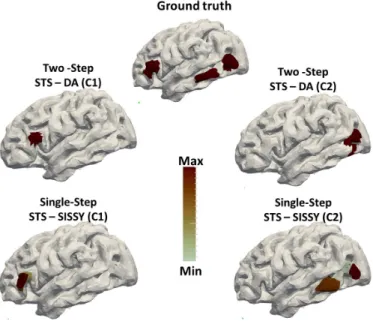
Figure 1 shows the estimated source distributions associ-ated with the two CP components for the tested single-step and two-step source localization algorithms for the second scenario (InfFr, MidTe, OccTe). For all algorithms, it can be seen that the patch InfFr may be associated with the first CP component whereas the patches MidTe and OccTe, that emit highly correlated signals, are combined in the second CP component. The patch InfFr is well delineated by both the
TABLE I. DLEAND EXECUTION TIME OF SOURCE IMAGING ALGORITHMS FOR SCENARIO1 (OCCSUP, SUPFR, INFFR)AND SCENARIO
2 (INFFR, MIDTE, OCCTE)
DLE (in cm) CPU time (in sec) scenario 1 2 1 2 Single step (STS-SISSY) 1.32 1.37 75.5 78.5
Two-step (STS-DA) 18.23 7.29 238.0 240.0
single-step approach and the two-step STS-DA method. The patches MidTe and OccTe, on the other hand, are only well localized by the single-step algorithm which clearly shows two distinct source regions associated with the second CP component. STSDA identifies a single patch in this case -located between patches MidTe and OccTe. Note that similar behavior was observed for these methods in the case of the second scenario.
Fig. 1. Scenario 2. (Top) from left to right: patches InfFr and patches MidTe and OccTe with highly correlated signals. (Bottom) source localization results for both CP components obtained with the different tested algorithms. C1 stands for the first CP component while C2 denotes the second one.
V. CONCLUSION
We have proposed a new source imaging algorithm that permits to separate and localize extended EEG sources in a single step. To do so, we have employed a tensor decomposi-tion approach which takes into account structural constraints by making use of the ALS and the ADMM optimization strategies. Simulations conducted using realistic EEG data, in the context of drug-resistent epilepsy, have shown that the proposed single-step approach provides the best localization accuracy and execution time compared to the classical two-step tensor-based source localization approach.
ACKNOWLEDGMENT
The work of R. Gribonval was funded by the FP7 European Research Council Programme, PLEASE project, under grant ERC-StG-2011-277906.
REFERENCES
[1] J. M¨ocks, “Decomposing event-related potentials: a new topographic components model,” Biological Psychology, vol. 26, pp. 199–215, 1988. [2] F. Miwakeichi, E. Martinez-Montes, P. A. Valdes-Sosa, N. Nishiyama, H. Mizuhara, and Y. Yamaguchi, “Decomposing EEG data into space-time-frequency components using parallel factor analysis,” NeuroImage, vol. 22, pp. 1035–1045, 2004.
[3] M. Morup, L. K. Hansen, C. S. Herrmann, J. Parnas, and S. M. Arnfred, “Parallel factor analysis as an exploratory tool for wavelet transformed event-related EEG,” NeuroImage, vol. 29, pp. 938–947, 2006. [4] M. De Vos, L. De Lathauwer, V. Vanrumste, S. Van Huffel, and W. Van
Paesschen, “Canonical decomposition of ictal scalp EEG and accurate source localisation: Principles and simulations study,” Computational Intelligence and Neuroscience, 2007.
[5] W. Deburchgraeve, P. J. Cherian, M. De Vos, R. M. Swarte, J. H. Blok, G. H. Visser, P. Govaert, and S. Van Huffel, “Neonatal seizure localization using Parafac decomposition,” Clinical Neurophysiology, vol. 120, pp. 1787–1796, 2009.
[6] M. Weis, D. Jannek, F. R¨omer, T. G¨unther, M. Haardt, and P. Husar, “Multi-dimensional PARAFAC2 component analysis of multi-channel EEG data including temporal tracking,” in IEEE Proc. of EMBC, Buenos Aires, Argentina, 2010.
[7] M. Morup, L. K. Hansen, S. M. Arnfred, L.-H. Lim, and K. H. Madsen, “Shift-invariant multilinear decomposition of neuroimaging data,” NeuroImage, vol. 42, no. 4, pp. 1439–1450, Aug. 2008. [8] B. Hunyadi, D. Camps, L. Sorber, W. Van Paesschen, M. De Vos,
S. Van Huffel, and L. De Lathauwer, “Block term decomposition for modelling epileptic seizures,” EURASIP Journal on Advances in Signal Processing, vol. 139, 2014.
[9] H. Becker, P. Comon, L. Albera, M. Haardt, and I. Merlet, “Multi-way space-time-wave-vector analysis for EEG source separation,” Signal Processing, vol. 92, pp. 1021–1031, 2012.
[10] H. Becker, L. Albera, P. Comon, M. Haardt, G. Birot, F. Wendling, M. Gavaret, C. G. B´enar, and I. Merlet, “EEG extended source local-ization: tensor-based vs. conventional methods,” NeuroImage, vol. 96, pp. 143–157, Aug. 2014.
[11] H. Becker, L. Albera, P. Comon, R. Gribonval, and I. Merlet, “Fast, variation-based methods for the analysis of extended brain sources,” in Proc. of EUSIPCO, Lisbon, Portugal, 2014.
[12] R. Bro, “Multi-way analysis in the food industry: Models, algorithms and applications,” Ph.D. dissertation, University of Amsterdam (NL), 1998.
[13] D. Gabay and B. Mercier, “A dual algorithm for the solution of nonlinear variational problems via finite elements approximations,” Computers and Mathematics with Applications, vol. 2, pp. 17–40, 1976. [14] R. Glowinski and A. Marrocco, “Sur l’approximation, par ´el´ements finis d’ordre un, et la r´esolution, par p´enalisation-dualit´e, d’une classe de probl`emes de dirichlet non lin´eaires,” Revue Franc¸aise d’Automatique, Informatique, et Recherche Op´erationelle, vol. 9, pp. 41–76, 1975. [15] A. P. Liavas and N. D. Sidiropoulos, “Parallel algorithms for constrained
tensor factorization via the alternating direction method of multipliers,” submitted to IEEE Transactions on Signal Processing, 2015. [16] N. D. Sidiropoulos, A. Liavas, and K. Huang, “Two takes on constrained
CP decomposition using the alternating direction method of multipliers.” [17] A. Gramfort, “Mapping, timing and tracking cortical activations with MEG and EEG: Methods and application to human vision,” Ph.D. dissertation, Telecom ParisTech, 2009.
[18] L. Albera, H. Becker, A. Karfoul, R. Gribonval, A. Kachenoura, L. Senhadji, A. Hernandez, and I. Merlet, “Localization of spatially distributed brain sources after a tensor-based preprocessing of interictal epileptic eeg data,” to appear in Proc. 37th International Conference of the IEEE Engineering in Medicine and Biology Society, 2015. [19] L. Ding, “Reconstructing cortical current density by exploring
sparse-ness in the transform domain,” Physics in Medicine and Biology, vol. 54, pp. 2683 – 2697, 2009.
[20] J. J. Moreau, “Fonctions convexes duales et points proximaux dans un espace hilbertien,” CR Acad. Sci. Paris S´er. A Math, vol. 255, pp. 2897– 2899, 1962.