Bayesian Image Restoration under Poisson Noise and Log-concave Prior

HAL Id: hal-02438049

https://hal.archives-ouvertes.fr/hal-02438049

Submitted on 14 Jan 2020

HAL is a multi-disciplinary open access

archive for the deposit and dissemination of

sci-entific research documents, whether they are

pub-lished or not. The documents may come from

teaching and research institutions in France or

abroad, or from public or private research centers.

L’archive ouverte pluridisciplinaire HAL, est

destinée au dépôt et à la diffusion de documents

scientifiques de niveau recherche, publiés ou non,

émanant des établissements d’enseignement et de

recherche français ou étrangers, des laboratoires

publics ou privés.

Bayesian Image Restoration under Poisson Noise and

Log-concave Prior

Maxime Vono, Nicolas Dobigeon, Pierre Chainais

To cite this version:

Maxime Vono, Nicolas Dobigeon, Pierre Chainais.

Bayesian Image Restoration under Poisson

Noise and Log-concave Prior. ICASSP 2019 - 2019 IEEE International Conference on Acoustics,

Speech and Signal Processing (ICASSP), May 2019, Brighton, United Kingdom.

pp.1712-1716,

�10.1109/ICASSP.2019.8683031�. �hal-02438049�

BAYESIAN IMAGE RESTORATION UNDER POISSON NOISE AND LOG-CONCAVE PRIOR

Maxime Vono, Nicolas Dobigeon

University of Toulouse, INP-ENSEEIHT

IRIT, CNRS, Toulouse, France

Pierre Chainais

University of Lille, CNRS, Centrale Lille

UMR 9189 - CRIStAL, Lille, France

ABSTRACT

In recent years, much research has been devoted to the restoration of Poissonian images using optimization-based methods. On the other hand, the derivation of efficient and general fully Bayesian approaches is still an active area of research and especially if stan-dard regularization functions are used, e.g. the total variation (TV) norm. This paper proposes to use the recent split-and-augmented Gibbs sampler (SPA) to sample efficiently from an approximation of the initial target distribution when log-concave prior distributions are used. SPA embeds proximal Markov chain Monte Carlo (MCMC) algorithms to sample from possibly non-smooth log-concave full conditionals. The benefit of the proposed approach is illustrated on several experiments including different regularizers, intensity levels and with both analysis and synthesis approaches.

Index Terms— Bayesian inference, image restoration, Poisson

noise, split-and-augmented Gibbs sampler.

1. INTRODUCTION

Poisson noise can appear in a lot of image processing problems where observations are obtained through a count of particles (e.g. photons) emitted by the object of interest and arriving in the im-age plane where a detector (e.g. a charged coupled device (CCD) camera) is located [1]. For instance, this statistical property of the noise occurs in emission tomography (ET) [2], fluorescence mi-croscopy [3] or astronomy [4, 5]. In particular, a growing interest in restoring astronomical Poissonian images can be traced back at least to the Hubble Space Telescope optical aberration in the early 90’s. Methods to tackle such image restoration problems in these years were mainly based on Tikhonov-Miller inverse filter and maximum likelihood (ML) estimation via the expectation-maximization (EM) algorithm [2, 6, 7]. This is for instance the case for the classical Richardson-Lucy algorithm [8, 9] used and revisited in a lot of ap-plications [10, 11] since noise amplification tended to appear. We refer the interested reader to [12] for a review of Poissonian image restoration methods up to 2006. Since then, much research has been devoted to these problems and a lot of advances have been made in optimization-based methods. Among other works, [13] considered a forward-backward splitting algorithm using the Anscombe vari-ance stabilizing transform (VST) [14] while [15–17] used alternate minimization schemes in order to tackle the exact Poissonian like-lihood function. The optimization-based algorithms derived by the aforementioned authors appear to be efficient in various scenarios ranging from analysis to synthesis approaches [18] with different regularization functions (e.g. total variation (TV) [19] or ℓ1norm) in low or high signal-to-noise ratio (SNR) cases.

On the other hand, Poissonian image restoration with fully Bayesian approaches, such as Markov chain Monte Carlo (MCMC)

methods, has not benefited from these recent advances in opti-mization making them less attractive. In particular, their high computational cost compared to variational methods can be pro-hibitive in high-dimensional applications (e.g. in astronomy) where the size of the observations can be of the order of the megapixel (resp. megavoxel). As a result, few efficient simulation-based methods exist to tackle image restoration under Poisson noise. For instance, [20, 21] dealt with the Poissonian likelihood by using a Taylor series expansion leading to a quadratic approximation of the former. In a similar vein, [22] used a Metropolis-within-Gibbs algorithm with a Gaussian proposal while the Riemmanian manifold Hamiltonian Monte Carlo method [23] has been proposed in [24]. Finally, a recent MCMC approach has been proposed in [25] ex-ploiting the Poisson-Gamma conjugacy which appears to compete with standard regularization functions such as TV.

However, up to our knowledge, no fully Bayesian approach con-sidered the sampling from a posterior distribution built on a Poisso-nian likelihood and standard convex and possibly non-smooth reg-ularizers. This paper proposes an approach relying on the recent split-and-augmented Gibbs sampler (SPA) [26] to tackle this prob-lem. In particular, the log-concave property of the prior permits to derive log-concave full conditionals that can be sampled by proxi-mal MCMC algorithms [27, 28] which rely on proximity operators of convex funtions. This approach permits to fulfill a number of important criteria for the practitioner. It yields good and reliable reconstruction results, a moderate computational time compared to optimization-based methods, the computation of credibility intervals and the ability to approximate several Bayesian estimators in a single run.

To this purpose, Section 2 presents the considered image pro-cessing problem and the main sampling issues associated to the de-rived posterior. Section 3 presents how SPA can handle complicated probability distributions of the form (7) with an approximate but controlled sampling scheme. Then, Section 4 derives SPA for the considered Poissonian image restoration problem where full con-ditionals are sampled using efficient state-of-the-art MCMC meth-ods. The proposed approach is illustrated on several experiments and compared to its determistic counterpart described in [16] as well as to the proximal Moreau-Yoshida unadjusted Langevin algorithm (P-MYULA) [28] although its direct application is not straightfor-ward and necessitates approximation schemes. Finally, Section 5 draws concluding remarks.

2. PROBLEM FORMULATION

This section presents the Bayesian inference problem related to Poissonian observations with a log-concave prior distribution. The main properties of the derived posterior distribution are presented before giving a brief review of existing Markov chain Monte Carlo (MCMC) methods that could be used to sample from this posterior.

2.1. Model

In this section, we consider the observation of some image y∈ Nm_,

damaged (e.g. blurred or with missing pixels) and contaminated by Poisson noise. We assume that each individual observation yi, i∈

J1, mK corresponds to an independent realization of a Poisson ran-dom variable, that is for all i∈ J1, mK,

yi

i.i.d.

∼ P([Hx + b]i

)

, (1)

where x∈ Rd+stands for an original image to recover, H∈ Rm×d is an operator related to the point spread function (PSF) and b∈ Rd

+ stands for some background noise, e.g. accidental coincidences in positron emission tomography (PET). We assume in the sequel that for all x∈ Rd+, Hx∈ Rd+. In order to make an easier link with the proposed approach, the likelihood distribution is rewritten as follows

p(y|x) ∝ exp(−f1(Hx; y)), (2) where f1(Hx; y) = m ∑ i=1 −yilog ( [Hx + b]i ) + [Hx + b]i. (3)

Following a Bayesian approach [29], the prior distribution is de-fined as follows for all x∈ Rd,

p(x)∝ exp(−f2(x)− f3(x)), (4) where f2(x) = τ ψ(x) and f3(x) = ι_Rd

+(x), (5)

where ψ : Rd → R stands for a proper, coercive, convex, lower semicontinuous (l.s.c), possibly non-differentiable function, τ is a positive parameter; ιCis the indicator function of setC, i.e. ιC(x) = 0 if x∈ C and ιC(x) = +∞ otherwise. The functions f2(via ψ) and f3 being convex, the potential f2+ f3 is also convex and the prior in (4) is log-concave. The function f2stands for some regu-larization term (e.g. ℓ1 norm) while the function f3guarantees the non-negativity of the original image x since the latter can be viewed as an intensity. By the application of Bayes’ rule, the posterior dis-tribution writes

π(x)∝ exp(−f1(Hx)− f2(x)− f3(x) )

, (6) and has the following properties stated by Proposition 1.

Proposition 1. 1. The posterior distribution π is log-concave. 2. The potential function f = f1+ f2+ f3 associated to π is

proper, l.s.c, coercive and convex. Additionally, if yi̸= 0 for

all i∈ J1, mK, f is strictly convex.

3. The negative log-likelihood function f1is differentiable but is

not gradient-Lipschitz continuous.

Proof. The proof of these properties follows directly from [16].

2.2. Related work

Up to our knowledge, no previous work considered the direct or ap-proximate sampling from the posterior distribution π defined in (6). Following Proposition 1,− log π is convex and possibly not dif-ferentiable. In this setting, since− log π is not differentiable, one could not resort to Hamiltonian Monte Carlo (HMC) methods [30] to sample from π. These methods were for instance resorted to sam-ple from π with f2 = f3 = 0 in [24]. Then, one could think

of using proximal MCMC approaches [27, 28] to tackle the non-differentiability of the potential function associated to π thanks to Moreau-Yoshida regularization [31]. However, these approaches re-quire the existence of a smooth gradient-Lipschitz continuous term in the potential function which is not the case in the problem consid-ered, see property 3 in Prop. 1. Note that it is possible to tackle this issue by using the Anscombe variance stabilizing transform [14], see Section 4. Additionally, proximal MCMC algorithms assume that the proximal operator associated to the non-smooth potential, here f2 + f3, is available. This is not the case for the considered potentials defined in (5) if one considers a synthesis frame-based approach, see Section 4.1. Therefore, one has to resort to a more complicated scheme (e.g. the splitting method of maximal mono-tone operators [32,33]) to compute this proximity operator. To avoid the above issues, the considered sampling problem is dealt with by resorting to a variable-splitting inspired MCMC algorithm, namely the split-and-augmented Gibbs sampler (SPA, see Section 3) that we recently proposed in [26]. Then, each full conditional distribution involves a smooth gradient-Lipschitz continuous potential function along with a possibly non-smooth potential enabling the use of prox-imal MCMC for each of them.

3. SPLIT-AND-AUGMENTED GIBBS SAMPLER This section presents a particular type of variable splitting-inspired hierarchical Bayes models in order to solve the inference problem presented in Section 2.1. The associated joint distribution, namely the split-and-augmented distribution is presented along with its main properties and will be targetted by SPA. In the sequel, the object x to infer is not necessarily the original image (e.g. x could be coef-ficients associated to a frame). Thereby, in order to embed a large number of cases, the variable splitting-based approach is presented below under a general formulation.

3.1. Hierarchical Bayes model

Let us start from the initial target distribution π under the very gen-eral form π(x)∝ exp  −∑b i=1 fi(Kix)   , (7)

where for all i ∈ {1, . . . , b}, Ki ∈ Rdi×d stands for a possible

operator (e.g. blur, decimation, wavelet transform) acting initially on x. We consider the variable splitting-inspired approach of [26]. We introduce some splitting and auxiliary variables z1:b∈ Rdi_and

u1:b ∈ Rdi, respectively. The new joint target distribution πρ,α is

defined as follows πρ,α(x, z1:b, u1:b)∝ exp  −∑b i=1 fi(zi) +φ1(Kix, zi− ui) + φ2(ui) ) , (8) where φ1, φ2 are two divergence functions such that πρ,α

de-fines a proper probability distribution. In the sequel, we choose the following forms for these two functions for all x, zi and

ui, φ1(Kix, zi − ui) = (2ρ2)−1 Kix− (zi− ui)

2 2 and

φ2(ui) = (2α2)−1∥ui∥22, where ρ, α > 0. This choice stems from the fact that φ1 is a convex, lower bounded, continuously differentiable and gradient Lipschitz function preluding the use of

proximal MCMC algorithms to sample from each full conditional distribution of πρ,αwithin a Gibbs sampling scheme. Additionally,

the quadratic form for φ2was chosen for conjugacy properties with

φ1. The properties of the split-augmented distribution πρ,αdefined

in (8) are presented in Proposition 2.

Proposition 2. Assume that the potential function associated to π

in (7) is proper, convex, l.s.c and coercive. Then

1. the full conditional distributions under πρ,αare log-concave

with a lower-bounded, smooth gradient Lipschitz continuous potential term along with a proper and l.s.c term.

2. in the limiting case ρ→ 0, the marginal distribution associ-ated to x under πρ,αcoincides with π.

Proof. The proofs corresponding to each property can be easily

derived using the fact that a l.s.c and coercive function is lower-bounded and by using the proof of [26, Theorem 1].

3.2. Gibbs sampler

Since sampling from π could be not straightforward with the exist-ing MCMC approaches (see Section 2.2), the samplexist-ing from πρ,αis

considered through the Gibbs sampler SPA [26] which targets alter-natively each full conditional distribution namely for all i∈ J1, bK

πρ,α(zi|x, ui)∝ exp  −fi(zi)− Kix− (zi− ui) 2 2 2ρ2   (9) πρ,α(ui|x) ∝ exp  −∥ui∥2₂ 2α2 − Kix− (zi− ui) 2 2 2ρ2   (10) πρ,α(x|zi, ui)∝ exp  −∑b i=1 Kix− (zi− ui) 2 2 2ρ2   . (11)

The associated sampling details are presented hereafter depending on the form of each full conditional.

Log-concave full conditionals –To begin with, the full condition-als associated to the splitting variables z1:bare log-concave with a smooth gradient Lipschitz term (related to φ1) and can be efficiently sampled using the proximal Moreau-Yoshida unadjusted Langevin algorithm (P-MYULA) if the proximity operators of f1:bare avail-able or can be approximated.

Gaussian full conditionals –On the other hand, the full condi-tional distribution associated with the variable of interest x is now Gaussian due to φ1 with a possibly non-diagonal covariance ma-trix. However, in cases where the matrices Ki are either

diago-nal or block-circulant, one can resort to the Fourier domain and to the Sherman-Morrison-Woodbury formula to re-write this covari-ance matrix with diagonal matrices. Then, the exact perturbation-optimization (E-PO) algorithm [34] can be used to sample efficiently the full conditional distribution associated to x. Additionally, the full conditionals associated to the auxiliary variables u1:bare Gaussian with diagonal covariance matrices and can be sampled efficiently even in high dimension.

4. APPLICATION TO POISSONIAN IMAGE RESTORATION

This section illustrates the proposed approach on Poissonian image restoration problems with either an analysis or a synthesis approach.

4.1. Applying SPA

Two image processing problems under Poisson noise without back-ground emission (i.e. b = 0d) are considered, namely image

deblur-ring with total variation (TV) prior and Laplacian prior combined with a frame-based approach. However, note that the proposed ap-proach can be generalized to other log-concave prior distributions. Image deblurring with TV prior –In this approach (denoted TV in table 1), the operators defined in Section 3.1 are K1= P, K2 =

K3 = Idand the object to recover is the original image x ∈ Rd+.

The matrix P is related to a Gaussian blurring kernel, hence is block-circulant and diagonalizable in the Fourier domain. The potential functions f1:3are those defined in Section 2.1 with ψ corresponding to the TV regularization function.

Frame-based synthesis approach –In this synthesis approach (de-noted WT for wavelet transform in table 1), the operators defined in Section 3.1 are K1 = PW, K2 = Id, K3= W and the object to

recover is the coefficients vector β associated to a frame such that

x = Wβ. The matrix P is related to a Gaussian blurring kernel and

the columns of W are the elements of the considered frame (e.g. wavelets or curvelets). In the sequel, the Haar wavelet frame with four levels is used. Obviously, depending on the image processing problem, one can consider more sophisticated frames. The potential functions f1:3are those defined in Section 2.1 with ψ corresponding to the ℓ1norm applied on β.

For these two approaches, the proximity operators associated to f1:3 can be computed using the closed-form expressions or approxima-tions detailed in [16].

4.2. Experimental setup

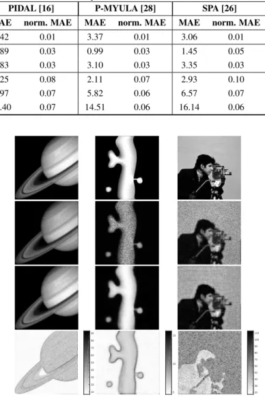
The proposed approach is illustrated on three blurred and Poisson contaminated images depicted on fig. 1. These images are of dif-ferent sizes, have a difdif-ferent maximum intensity level M and are restored using either the TV prior (TV) or using a synthesis ap-proach with wavelets (WT), see table 1. The proposed apap-proach is compared with the Poisson image deconvolution by augmented Lagrangian (PIDAL) algorithm [16] which stands for a particular in-stance of the alternating direction method of multipliers (ADMM). Note that the latter can be viewed as a deterministic counterpart of the proposed approach. Although, it cannot be directly applied to sample from (7) (see Section 2.2), the proximal MCMC algorithm P-MYULA has also been implemented by using the Anscombe VST and Douglas-Rachford splitting method to compute the proximity operator of f2+ f3when a frame-based synthesis approach is used. Note that we consider this as an interesting side contribution of this paper. We ran each MCMC algorithm with TMC = 105 for SPA (resp. 106for P-MYULA due to slower mixing properties) iterations and 104 _{samples were used in both cases to approximate Bayesian} estimators. SPA parameters have been set to (ρ, α) = (1, 1) as a trade-off between good reconstruction results and mixing proper-ties, see [26] for more details on the choice of these two parameters. Since the ground-truth is known in the considered experiments, the performance of each method has been assessed using the mean abso-lute error (MAE = d−1∥ˆx − x∥₁) and its normalized version (norm. MAE) with respect to (w.r.t.) the intensity level M . Note that the MAE is particularly relevant for Poissonian restoration since it is re-lated to other distances [13,35]. For each method, these criteria have been averaged on 10 independent runs.

Table 1. Poissonian image restoration with log-concave priors. Performance results for both optimization and simulation-based algorithms averaged over 10 runs. For the MCMC algorithms, the MMSE estimate has been used to compute the relative and normalized MAE criteria.

PIDAL [16] P-MYULA [28] SPA [26] image size approach M τ MAE norm. MAE MAE norm. MAE MAE norm. MAE Saturn 256× 256 TV 300 (Fig. 1) 0.1 2.42 0.01 3.37 0.01 3.06 0.01 neuron 128× 128 TV 30 (Fig. 1) 1 0.89 0.03 0.99 0.03 1.45 0.05 100 1 2.83 0.03 3.10 0.03 3.35 0.03 cameraman 128× 128 WT 30 0.1 2.25 0.08 2.11 0.07 2.93 0.10 100 0.1 6.97 0.07 5.82 0.06 6.57 0.07 255 (Fig. 1) 0.1 17.40 0.07 14.51 0.06 16.14 0.06 4.3. Results

Performance results – Table 1 shows the performance of each method on six different experiments. The standard deviation associ-ated to each tuple (experiment/norm. MAE) is roughly of the order of 0.005. For MCMC algorithm the minimum mean square error (MMSE) estimate has been used to compute MAE criteria. The re-sults of the proposed approach are close to the two other approaches although each method has a different target. Indeed, PIDAL derives the maximum a posteriori (MAP) estimate associated to (7) while P-MYULA and SPA were resorted here to compute MMSE estimates (obviously, other Bayesian estimates can be computed). In addition, we would like to emphasize that although SPA targets an approxi-mate probability distribution, the approximation is controlled with a single parameter ρ that can be made arbitrarily small, see Propo-sition 2. On the contrary, P-MYULA suffers here from a lot of approximations namely the absence of accept/reject step, the use of the Anscombe VST and the Douglas-Rachford splitting scheme to compute the proximity operator of f2+ f3for frame-based ap-proaches. Although the first approximation can be controlled with a single parameter [28], the second one is not justified in all scenarios and the last one implies an additional computational cost since it is iterative. For information, SPA was in average at least 6 times faster in terms of computational time than P-MYULA in the considered experiments.

Credibility intervals –Additionally to compute pointwise Bayesian estimates (e.g. MMSE estimate, see fig. 1), the proposed approach has the benefit of proposing credibility intervals by exploring the whole posterior distribution of the variable of interest x.

Thus, fig. 1 shows the 95% credibility intervals computed by SPA for a couple of experiments. For the cameraman and Saturn images, one can remark that the credibility intervals associated to highly Poisson contaminated regions appear to have a noise struc-ture. On the other hand, the range of credibility intervals associated to the neuron image are roughly piecewise constants. This difference is mainly due to the amount of regularization (via the parameter τ ) set for each image. Indeed, for the cameraman and Saturn image, τ was smaller since more details were present in the image. As pointed out by [28], we believe that simulation and optimization-based algo-rithms should be considered together to conduct image processing and analysis tasks. Indeed, first a quick MAP estimation can be per-formed by optimization techniques with standard regularizers. Then, the proposed approach can be used to conduct uncertainty quantifica-tion, hypothesis testing or even model selection by comparing model evidences since the potential of the target πρ,αin (8) corresponds to

an arbitrary small approximation of the initial potential function.

10 20 30 40 50 60 70 80 90 5 10 15 20 30 40 50 60 70 80 90 100 110

Fig. 1. Original images (1st row), noisy and blurred observations (2nd row), MMSE estimates computed with SPA (3rd row) and as-sociated 95% credibility intervals (4th row).

5. CONCLUSION

This paper derives a novel MCMC approach to restore Poissonian images under a log-concave prior distribution. Along with efficient optimization-based algorithms, the proposed approach has the ben-efit of completing the inference task by providing uncertainty quan-tification or by performing model selection. Moreover, the proposed approach has reasonable computation time w.r.t. optimization-based methods thanks to the embedding of efficient proximal MCMC algo-rithms. This work paves the way toward efficient fully Bayesian ap-proaches for even more complicated models (e.g. Poisson-Gaussian noise) or richer models using sophisticated regularization functions (e.g. total generalized variation).

6. REFERENCES

[1] M. Bertero et al., “Image deblurring with Poisson data: from cells to galaxies,” Inverse Problems, vol. 25, no. 12, 2009. [2] L. A. Shepp and Y. Vardi, “Maximum likelihood

reconstruc-tion for emission tomography,” IEEE Trans. Med. Imag., vol. 1, no. 2, pp. 113–122, Oct 1982.

[3] D. A. Agard and J. W. Sedat, “Three-dimensional architecture of a polytene nucleus,” Nature, vol. 302, pp. 676–681, 1983. [4] R. J. Hanisch and R. L. White (ed.), “The restoration of HST

images and spectra,” 1991.

[5] R. J. Hanisch and R. L. White (ed.), “The restoration of HST images and spectra II,” 1994.

[6] M. Bertero et al., “Three-dimensional image restoration and super-resolution in fluorescence confocal microscopy,” Journal

of Microscopy, vol. 157, no. 1, pp. 3–20, January 1990.

[7] T. J. Holmes, “Maximum-likelihood image restoration adapted for noncoherent optical imaging,” J. Opt. Soc. Am. A, vol. 5, no. 5, pp. 666–673, May 1988.

[8] W. H. Richardson, “Bayesian-based iterative method of image restoration,” J. Opt. Soc. Am., vol. 62, no. 1, pp. 55–59, Jan 1972.

[9] L. B. Lucy, “An iterative technique for the rectification of ob-served distributions,” Astron. J., vol. 79, pp. 745–754, 1974. [10] J.-L. Starck, A. Bijaoui, and F. Murtagh, “Multiresolution

sup-port applied to image filtering and deconvolution,” vol. 57, pp. 420–431, 01 1995.

[11] N. Dey et al., “Richardson-Lucy algorithm with total variation regularization for 3D confocal microscope deconvolution,”

Mi-crosc. Res. Tech., vol. 69, no. 4, pp. 260–266, April 2006.

[12] P. Sarder and A. Nehorai, “Deconvolution methods for 3-D fluorescence microscopy images,” IEEE Signal Process. Mag., vol. 23, no. 3, pp. 32–45, May 2006.

[13] F. Dup´e, J. M. Fadili, and J. Starck, “A proximal iteration for deconvolving Poisson noisy images using sparse representa-tions,” IEEE Trans. Image Process., vol. 18, no. 2, pp. 310– 321, Feb 2009.

[14] F. J. Anscombe, “The transformation of Poisson, binomial and negative-binomial data,” Biometrika, vol. 35, pp. 246–254, 1948.

[15] N. Pustelnik, C. Chaux, and J. Pesquet, “Parallel proximal algorithm for image restoration using hybrid regularization,”

IEEE Trans. Image Process., vol. 20, no. 9, pp. 2450–2462,

Sept 2011.

[16] M. A. T. Figueiredo and J. M. Bioucas-Dias, “Restoration of Poissonian images using alternating direction optimization,”

IEEE Trans. Image Process., vol. 19, no. 12, pp. 3133–3145,

2010.

[17] F.-X. Dup´e, M. Fadili, and J.-L. Starck, “Deconvolution under Poisson noise using exact data fidelity and synthesis or analysis sparsity priors,” Statistical Methodology, vol. 9, no. 1, pp. 4 – 18, 2012.

[18] M. Elad, P. Milanfar, and R. Rubinstein, “Analysis versus syn-thesis in signal priors,” vol. 23, pp. 947–968, 2007.

[19] L. I. Rudin, S. Osher, and E. Fatemi, “Nonlinear total variation based noise removal algorithms,” Phys. Rev. D, vol. 60, no. 1-4, pp. 259–268, Nov. 1992.

[20] M. Howard, A. Luttman, and M. Fowler, “Sampling-based uncertainty quantification in deconvolution of X-ray radio-graphs,” J. Comput. Appl. Math., vol. 270, pp. 43 – 51, 2014. [21] M. J. Fowler et al., “A stochastic approach to quantifying the

blur with uncertainty estimation for high-energy X-ray imag-ing systems,” Inverse Probl. Sci. Eng., vol. 24, no. 3, pp. 353– 371, 2016.

[22] J. M. Bardsley and A. Luttman, “A Metropolis-Hastings method for linear inverse problems with Poisson likelihood and Gaussian prior,” Int. J. Unc. Quant, vol. 6, no. 1, pp. 35–55, 2016.

[23] M. Girolami and B. Calderhead, “Riemann manifold Langevin and Hamiltonian Monte Carlo methods,” vol. 73, no. 2, pp. 123–214, March 2011.

[24] S. Pedemonte, C. Catana, and K. Van Leemput, “Bayesian tomographic reconstruction using Riemannian MCMC,” in

Med. Image Comp. Computer-Assisted Intervention (MICCAI),

2015.

[25] Y. Altmann et al., “A Bayesian approach to denoising of single-photon binary images,” IEEE Trans. Comput. Imag., vol. 3, no. 3, pp. 460–471, Sept 2017.

[26] M. Vono, N. Dobigeon, and P. Chainais, “Split-and-augmented Gibbs sampler - Application to large-scale inference problems,” submitted, 2018. [Online]. Available: https://arxiv.org/abs/1804.05809/

[27] M. Pereyra, “Proximal Markov chain Monte Carlo algorithms,”

Stat. Comput., vol. 26, no. 4, pp. 745–760, July 2016.

[28] A. Durmus, E. Moulines, and M. Pereyra, “Efficient Bayesian computation by proximal Markov chain Monte Carlo: When Langevin meets Moreau,” SIAM J. Imag. Sci., vol. 11, no. 1, pp. 473–506, 2018.

[29] C. P. Robert, The Bayesian Choice: a decision-theoretic

moti-vation. Springer, 2001.

[30] S. Duane et al., “Hybrid Monte Carlo,” Phys. Lett. B, vol. 195, no. 2, pp. 216 – 222, 1987.

[31] J. J. Moreau, “Fonctions convexes duales et points proximaux dans un espace Hilbertien,” C. R. Acad. Sci. Paris Ser. A Math., vol. 255, pp. 2897–2899, 1965.

[32] J. Eckstein and D. P. Bertsekas, “On the Douglas-Rachford splitting method and the proximal point algorithm for maxi-mal monotone operators,” Math Programm., vol. 55, no. 1, pp. 293–318, Apr 1992.

[33] P. Lions and B. Mercier, “Splitting algorithms for the sum of two nonlinear operators,” SIAM J. Numer. Anal., vol. 16, no. 6, pp. 964–979, 1979.

[34] G. Papandreou and A. L. Yuille, “Gaussian sampling by local perturbations,” in Adv. in Neural Information Process. Systems, 2010, pp. 1858–1866.

[35] A. R. Barron and T. M. Cover, “Minimum complexity density estimation,” IEEE Trans. Inf. Theory, vol. 37, no. 4, pp. 1034– 1054, July 1991.