HAL Id: hal-02944348
https://hal.archives-ouvertes.fr/hal-02944348
Submitted on 21 Sep 2020
HAL is a multi-disciplinary open access
archive for the deposit and dissemination of
sci-entific research documents, whether they are
pub-lished or not. The documents may come from
teaching and research institutions in France or
L’archive ouverte pluridisciplinaire HAL, est
destinée au dépôt et à la diffusion de documents
scientifiques de niveau recherche, publiés ou non,
émanant des établissements d’enseignement et de
recherche français ou étrangers, des laboratoires
Learning Obstacle Representations for Neural Motion
Planning
Robin Strudel, Ricardo Garcia, Justin Carpentier, Jean-Paul Laumond, Ivan
Laptev, Cordelia Schmid
To cite this version:
Robin Strudel, Ricardo Garcia, Justin Carpentier, Jean-Paul Laumond, Ivan Laptev, et al.. Learning
Obstacle Representations for Neural Motion Planning. CoRL 2020 - Conference on Robot Learning,
Nov 2020, Cambridge MA / Virtual, United States. �hal-02944348�
Learning Obstacle Representations
for Neural Motion Planning
Robin Strudel Inria∗ Ricardo Garcia Inria† Justin Carpentier Inria∗ Jean-Paul Laumond Inria∗ Ivan Laptev Inria∗ Cordelia Schmid Inria∗
Abstract: Motion planning and obstacle avoidance is a key challenge in robotics applications. While previous work succeeds to provide excellent solutions for known environments, sensor-based motion planning in new and dynamic environ-ments remains difficult. In this work we address sensor-based motion planning from a learning perspective. Motivated by recent advances in visual recognition, we argue the importance of learning appropriate representations for motion plan-ning. We propose a new obstacle representation based on the PointNet architec-ture [1] and train it jointly with policies for obstacle avoidance. We experimentally evaluate our approach for rigid body motion planning in challenging environments and demonstrate significant improvements of the state of the art in terms of accu-racy and efficiency.
Keywords: neural motion planning, obstacle avoidance, representation learning
1
Introduction
Motion planning is a fundamental robotics problem [2, 3] with numerous applications in mo-bile robot navigation [4], industrial robotics [5], humanoid robotics [6] and other domains. Sampling-based methods such as Rapidly Exploring Random Trees (RRT) [7] and Probabilistic Roadmaps (PRM) [8] have been shown successful for finding a collision-free path in complex en-vironments with many obstacles. Such methods are able to solve the so-called piano mover prob-lem [9] and typically assume static environments and prior knowledge about the shape and location of obstacles. In many practical applications, however, it is often difficult or even impossible to obtain detailed a-priori knowledge about the real state of environments. It is therefore desirable to design methods relying on partial observations obtained from sensor measurements and enabling motion planning in unknown and possibly dynamic environments. Moreover, given the high complexity de-voted to exploration in sampling-based methods, it is also desirable to design more efficient methods that use prior experience to quickly find solutions for motion planning in new environments. To address the above challenges, several works [10,11,12,13,14,15] adopt neural networks to learn motion planning from previous observations. Such Neural Motion Planning (NMP) methods either improve the exploration strategies of sampling-based approaches [13] or learn motion policies with imitation learning [12,15] and reinforcement learning [14]. In this work we follow the NMP paradigm and propose a new learnable obstacle representation for motion planning.
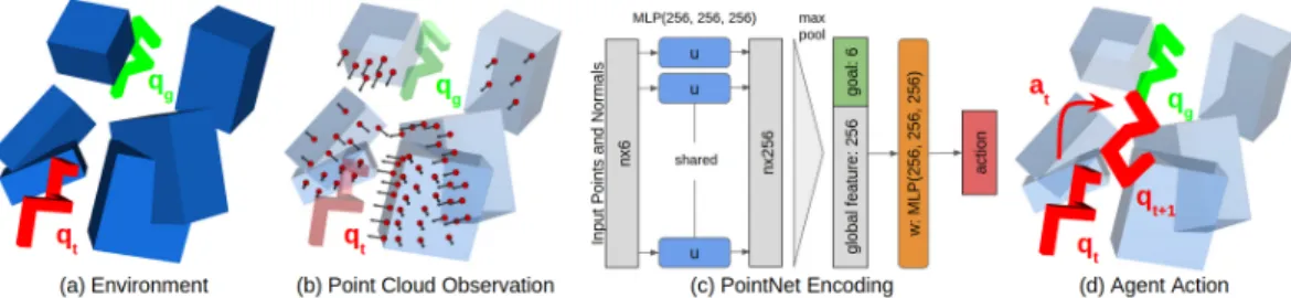
Motivated by recent advances in visual recognition [1,16,17], we argue that the design and learning of obstacle representations plays a key role for the success of learning-based motion planning. In this work, we proposed a new representation based on point clouds which are first sampled from visible surfaces of obstacles and then encoded with a PointNet [1] neural network architecture, see Fig. 1. We learn our obstacle representation jointly with the motion planing policies in the SAC (Soft Actor Critic) reinforcement learning framework [18]. In particular, while using envi-ronments composed of 3D-box shapes during training, we demonstrate the generalization of our
∗
Inria, ´Ecole normale suprieure, CNRS, PSL Research University, 75005 Paris, France.
†
University Grenoble Alpes, Inria, CNRS, Grenoble INP, LJK, 38000 Grenoble, France.
Figure 1: Overview of our approach. (a) We aim to find a collision-free path for a rigid body from its current configuration qtto the goal configuration qg. (b) We assume no prior knowledge about the scene and represent obstacles by points and normals sampled on object surfaces. (c) Our neural network learns the PointNet encoding of observed points and normals together with the motion policy. (d) The learned network generates actions that move the body towards the goal configuration along a collision-free path.
motion planning policies to complex environments with objects of previously unseen shapes. We also show our method to seamlessly generalize to new object constellations and dynamic scenes with moving obstacles. We evaluate our method in challenging simulated environments and vali-date our representation through ablation studies and comparison to the state of the art. Our method significantly improves the accuracy of previous NMP methods while being one order of magnitude more computationally efficient compared to close competitors.
The contributions of our work are threefold. First, we propose a new learnable obstacle representa-tion based on point clouds and the PointNet neural architecture [1]. Second, we learn our represen-tation jointly with policies for rigid body motion planning using reinforcement learning. Finally, we experimentally evaluate our approach and demonstrate significant improvements of the state of the art in motion planning in terms of accuracy and efficiency. Qualitative results along with a video are available on the project webpage [19].
2
Related Work
Sampling-based motion planning. Sampling-based methods such as RRT [7] have been exten-sively studied for motion planning [2,20,3,7,8]. Such methods can deal with complex environ-ments, however, they typically assume a complete knowledge of the robot workspace and static obstacles. Given the complexity of sampling-based methods, recent work proposes efficient explo-ration schemes [21,22,23,24], e.g., by reusing previously discovered paths in similar scenarios [23] or biasing RRT search to promising regions [24]. Our work does not assume any a-priori knowledge about the environment and can deal with moving obstacles. Moreover, while our method performs an extensive exploration during training, the learned policies directly generate feasible paths during testing in new environments.
Neural motion planning. Learning-based methods for motion planning have been introduced in [10,11]. Motivated by the success of deep learning, a number of more recent methods explore neural networks for motion planning and obstacle avoidance. Ichter et al. [13] learns to sample robot configurations close to the target RRT solutions. Qureshi et al. [15] and Pfeiffer et al. [12] learn a policy with the imitation learning using RRT solutions as demonstrations. While improving the efficiency of RRT, [12,13,15] still require sampling at test time and are not easily applicable in scenes with moving obstacles. Our work is most related to Jurgenson and Tamar [14] who ex-plore reinforcement learning (RL) to learn motion policies. Similar to [14] we use RL and learn to avoid obstacles using a negative collision reward. While [14] presents results in relatively simple 2D environments, we propose a new learnable obstacle representation that generalizes to complex 3D scenes. We experimentally compare our method to [13,14,15] and demonstrate improved accuracy. Visual Representation. The NMP methods [14,15,13] assume full knowledge of the workspace and use an obstacle encoding either based on a 2D image of obstacles encoded with a convolutional neural network (CNN) [14], or an occupancy grid [13] or a volumetric point cloud [15] encoded with a multi-layer perpeceptron (MLP). We show that obstacles representation is critical to solve complex problems with rich workspace variations and propose to rely on a point cloud representation of obstacles coupled with PointNet [1]. Qi et al. [1] demonstrated the performance of PointNet to classify and segment point clouds, in this work we propose to use it to encode obstacles.
3
Method
3.1 Overview of the method
In this work we consider rigid robots with 2 to 6 degrees of freedom (DoF). Let W ⊆ R3 be the workspace of the robot, containing a set of obstacles V. We denote Cf reethe open set of configu-rations where the robot does not collide with the obstacles V and Ccollision = C \ Cf ree. Given a start configuration q0∈ Cf reeand a goal configuration qg∈ Cf ree, motion planning aims at finding a collision-free path which connects the start configuration to the goal configuration. A continuous function τ : [0, 1] → C is a solution if τ ([0, 1]) is a subset of Cf ree, τ (0) = q0and τ (1) = qg. A motion planning problem is thus defined by a start configuration, a goal configuration and a set of obstacles V.
In this work, we represent obstacles V by sets of points (point clouds) and the corresponding nor-mals sampled on the surface of obstacles. This representation is valid for arbitrary shapes and can be obtained with a depth sensor. We consider the robot as an embodied agent which senses sur-rounding obstacles with a panoramic camera (Fig.1a). The point cloud, expressed in the robot local coordinate frame (Fig.1b), is then processed with a PointNet architecture [1] to encode the obstacles (Fig.1c). The goal vector qgis expressed in the robot local coordinate frame and is concatenated to the PointNet obstacle encoding. This vector is processed by a MLP that generates actions, bringing the robot closer to the goal while avoiding obstacles (Fig.1d). We learn the policy jointly with the PointNet encoding of the obstacles (Fig.1c) in an end-to-end fashion with reinforcement learning. In the next two sections, we first give details on the obstacle representation and then describe policy learning.
3.2 Obstacle representation for motion planning
We aim to learn a function that encodes the obstacles and the goal configuration as a vector en-abling subsequent motion planning. While many parametric functions could be used as an encoder, we follow advances in visual recognition [1,16,17] and define obstacle representations by a neu-ral network learned jointly with the task of motion planning. We experimentally demonstrate the significant impact of the encoder on the performance of motion planning in Section4.
In previous works [13,14,15], obstacles have been represented by occupancy grids encoded with a MLP [13,15] or images encoded with a CNN [14] assuming global workspace knowledge. In our work we use points sampled on the surface of obstacles along with their oriented normals. Such measurements can be obtained using a depth sensor either placed on the robot or at other locations. A set of obstacles V is represented by a finite set Snormals= {(xi, ni)}i=1,...,N∈ RN ×2d where d = 2, 3 and the points xiand normals niare expressed in the robot local coordinate frame. We denote by αi the couple (xi, ni). We define the goal g as the displacement to reach the goal configuration from the current robot configuration.
To process a point cloud, we use a PointNet [1] like network (Fig.1c) reduced to its core layers for computation efficiency which we describe below. The idea of PointNet is to use a function which is symmetric with respect to the input to get a model invariant to input permutations. Based on this idea we build a network composed of two MLPs u and w with Exponential Linear Units (ELUs) activation [25] as shown in Fig.1c. The first MLP u is shared across point cloud elements αi(Fig.1c blue block) and is used to generate local features of each element u(αi). Then, a max operation is applied to obtain a global feature v encoding the point cloud. The global feature v is further concatenated with the goal g (Fig.1c green block) and passed through a second MLP w (Fig.1c orange block):
v(α1, ..., αN) = max
i=1,...,N[u(α1), ..., u(αN)] f (α1, ..., αN, g) = w(v(α1, ..., αN), g)
(1)
The max operator is a max-pooling operation: given a list of feature vectors of size N × d, it outputs a vector of size d by taking the maximum over the N points in each coordinate.
The PointNet encoding of obstacles u is trained jointly with the policy w. For the training of u and w we compare imitation learning and reinforcement learning schemes as described in the next section.
3.3 Learning policies for motion planning
We cast the motion planning problem as a Markov decision process (MDP) [26]. The state space S is the configuration space of the robot C, A is the space of valid velocities at the current config-uration and O is a representation of the workspace along with the goal configconfig-uration g. Given a robot configuration q ∈ Cf reeand v an admissible velocity vector, we denote q(v) as the configu-ration reached by applying the velocity vector v to the robot for a fixed time. As the robot can hit into obstacles, we consider qf ree(v) which returns the last collision free configuration on the path connecting q to q(v). Then the dynamics p is defined as p(q, v) = qf ree(v).
We aim at learning policies to solve motion planning problems. For that purpose, we explore and compare policies trained with imitation learning (behavioral cloning) and reinforcement learning. To train a policy with imitation learning [27], we collect a dataset D = {(ot, at)} of observation-action pairs along expert trajectories generated with Bi-RRT [7] and follow the behavioral cloning approach [28]. Given a learnable policy π, we minimize the L2loss, L(π) = kat−π(ot)k2, between the expert action atand the policy applied to the expert observation ot.
To train a policy with reinforcement learning [26], we define a reward function as follows. Given a goal configuration g ∈ C, we define rvelocity(q, v) = −kvk2and
rtask(q, v, g) = rgoal if kqf ree(v) − gk ≤ ε, rf ree if [q, q(v)] ⊂ Cf ree, rcollision else. (2)
with rgoal > 0, rf ree < 0 and rcollision < 0. The reward function is then defined as r(q, v, g) = rvelocity(q, v) + rtask(q, v, g). rtask rewards actions reaching g and penalizes actions which lead to a collision. Given two collision-free paths leading to the goal, the total re-ward r(q, v, g) is highest for the shortest path. Maximizing the rere-ward enables the policy path to be collision free and as short as possible. Note that the dynamics p depends only on the robot and the workspace, and the reward function r depends additionally on the goal configuration to be reached. An episode is terminated when reaching the goal or the maximum number of steps.
The reward rtask defined above is sparse with respect to the goal: it is only positive if the agent reaches the goal during one episode, which may have a low probability in challenging environments. Hindsight Experience Replay (HER) [29] is a technique to improve the sample efficiency of off-policy RL algorithms in the sparse and goal-conditioned setting which we use extensively in this work. After collecting one rollout s0, ..., sT which may or may not have reached the goal g, it consists in sampling one of the states as the new goal g0 for this rollout. The rollout may not have reached g but in hindsight, it can be considered as a successful rollout to reach g0. HER can be seen as a form of implicit curriculum learning which accelerates the learning of goal-conditioned policies.
4
Experimental Results
Below we describe our experimental setup and implementation details in Sections4.1and4.2. Sec-tion4.3evaluates alternative obstacle representations while Sections 4.4and4.5compare our ap-proach to the state of the art in challenging environments.
4.1 Environments
We evaluate our method in a number of different environments, namely, 2D and 3D environments used in [13,15], our own 3D environments and an environment based on a classic motion planning problem [20] where a S-shape with 6 DoF should go through a thin slot. We consider rigid body robots which are either a 2D/3D sphere with 2/3 DoF or a S-shape body with 6 DoF. We use distinct workspaces for training and evaluation so that policies are evaluated on workspaces unseen during training. We evaluate the success rate of a policy over 400 rollouts. At the end of a rollout, the environment is reset: a new random workspace is sampled along with a start and goal configuration. A rollout is considered successful if it reaches a configuration near the goal defined by an epsilon neighborhood before the maximum number of steps is reached. We describe details for each of our environments below.
2D-Narrow [13]: we generate 2D environments from Ichter et al. [13] using publicly available code [30]. The environment contains a sphere robot navigating in 2D workspaces composed of 3
randomly generated narrow gaps as shown in Fig.2and random start and goal configurations. We set the maximum number of policy steps to 50.
3D-Qureshi [15]:3D workspaces with a sphere robot from Qureshi et al. [15] contain axis-aligned boxes with fixed center and varying sizes. We used open-source code from Qureshi [31] to generate the workspaces.
3D-Boxes:our environment composed of 3 to 10 static boxes generated with random sizes, positions and orientations as illustrated in Fig.4(a). The maximum number of steps is set to 80.
3D-Synthethic: a variant of 3D-Boxes composed of unseen synthetic obstacles such as capsules, cylinders and spheres instead of boxes as illustrated in Fig.4(b).
3D-YCB:a variant of 3D-Boxes composed of real objects from the YCB dataset [32] recorded with a RGB-D camera, see Fig.4(c).
3D-Dynamic:a variant of 3D-Boxes with dynamic obstacles moving in real time. For each box two placements are sampled uniformly and the current box placement is interpolated between the two. Slot:a S-shaped robot with 6 DoF which has to go through a thin gap with varying size, 2 times to 8 times wider than the smallest robot link. This is a classic problem in motion planning [20] illustrated in Fig.4(d).
4.2 Implementation details
Below we describe implementation details for our method and for other methods used for com-parison. To train policies with reinforcement learning, we use Soft Actor Critic (SAC) [18] with automatic entropy tuning, a learning rate of 3.10−4 with Adam optimizer [33], a batch size of 256 and a replay buffer of 106steps combined with Hindsight Experience Replay (HER) [29] with 80% of the trajectories goal relabeled, as in the original papers. We train a policy on 2.106environment steps before reporting the results. We use the open-source implementation of Pong [34]. To train policies with imitation learning, we use a learning rate of 10−3 with Adam optimizer [33] and a batch size of 256. For Bi-RRT, once a solution is found, we shorten its length by randomly sampling two points along the solution, if the shortcut made out of these two points is collision free we modify the solution to include it. The maximal size of an edge in RRT corresponds to the maximal size of a policy step for RL or BC, in this way computing collision checking on an edge has the same cost for both.
For the MLP network, we use 3 hidden layers of size 256. For the convolutional neural network (CNN), we use 3 convolutional layers with 32 filters of size 3 × 3 followed by a max-pooling operator and 3 hidden layers of size 256. For PointNet, we use 3 hidden layers of size 256 for the point encoder u and the global feature network w respectively. For the MLP, the goal is concatenated to the list of points. For the CNN, the current and goal configurations are concatenated to the feature vector after max-pooling.
For Ichter et al. [13], we used the code provided in [30] along with the dataset to train the conditional variational auto-encoder. Once trained we combined the learned sampling with Bi-RRT to report the results. For Qureshi et al. [15], we adjust the implementation provided by Qureshi [31] to our environments. We followed the training procedure described in [15]. For Qureshi neural replanning (NR), we run neural planning for 80 steps then use neural replanning recursively for 10 iterations each comprising 50 steps maximum. For Qureshi hybrid replanning (HR), if neural replanning fails to find a solution after 10 iterations, Bi-RRT is used to find a path between states where there is still a collision. For Jurgenson and Tamar [14], we adapted the open-source implementation [35] to run on our environment. For training, we use the same parameters as [14], image based workspace representation and reward definition. We follow their DDPG-MP method. The training dataset consists of 104 workspaces. For pre-training, we use 400 random steps per workspace and for training, we use Bi-RRT generated 10 expert trajectories per workspace.
Finally, the rigid bodies and obstacles are modeled using Pinocchio [36,37] and collision checks are computed by FCL [38].
4.3 Comparison of obstacle representations and learning approaches
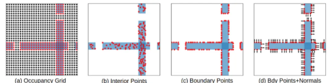
In this section we compare different policies on the 2D-Narrow environment [13]. Policies are trained with Behavioral Cloning (BC) or Reinforcement Learning (RL) using different obstacles representations presented in Fig.2. The occupancy grid is a 64 × 64 image (Fig.2a), the point clouds are composed of 128 points either sampled on the interior of obstacles (Fig.2b) or at their boundary (Fig.2c,2d). 128 points is a good trade-off between speed and accuracy as adding more points did
Figure 2: Illustration of different obstacles representations for 2D-Narrow. See Table1for results.
Behavioral Cloning Reinforcement Learning
64×64 Image - CNN 64.5% 44.5%
Interior points - MLP 42.0% 29.0%
Interior points - PointNet 76.0% 83.0%
Boundary points - PointNet 85.0% 93.8%
Boundary points and normals - PointNet 86.5% 99.5%
Table 1: Comparison of different obstacles representations and policies training methods on the 2D-Narrow environment.
not improve the results. In Table1, we report the success rate of RL policies after 1000 epochs which corresponds to 106interactions with the environment, a stage at which the policies performance have plateaued. For BC, we collect a dataset of solutions using Bi-RRT, containing 106steps in total and train for 200 epochs. This allows a fair comparison of BC and RL which have been trained on the same dataset size. As a baseline, we consider a policy which goes from start to goal in a straight line and has a success rate of 45.5%.
Table1 shows that the choice of obstacles representation greatly impacts the policy success rate both for BC and RL. Using a representation based on an occupancy grid encoded with a CNN yields poor performance for both BC and RL. Similarly, if interior points are encoded with a MLP the performance is low for both BC and RL. In both case results with RL are below BC. For BC, the training set is composed of expert demonstrations which is fixed for every representation. In contrast, as the RL training set is generated by the learning policy, the obstacles representation impacts the quality of the training set. Encoding interior points with PointNet results in a significant gain, +34% for BC and +54% for RL. Using PointNet in combination with boundary points and normals increases the performance by +10% for BC and +16% for RL. We can also observe that normals improve the performance over boundary points alone. Furthermore, with a more stable obstacle encoding, RL outperforms BC by a margin, +13% in the case of boundary points and normals.
Figure 3: (a) Vector field of a policy trained with behavioral cloning. (b) Vector field of a policy trained with reinforcement learning. (c) RL path samples. (d) RRT samples generated to find a path. The difference between policies trained with BC or RL is illustrated in Fig.3(a,b). For each policy, a vector field has been generated by using a grid covering the environment and computing the policy output at each point given a fixed goal plotted in red. We observe that policies trained with BC can fail close to edges of obstacles. This is a typical problem of imitation learning [39] which is limited to perfect, expert trajectories in the training set and does not observe failure cases. In contract, RL explores the environment during training and generates actions pointing away from obstacles as it has been trained explicitly to avoid collisions.
We compare our approach to state-of-the-art neural motion planning approaches [13,14,15] and Bi-RRT [7] in Table2. We compare in terms of success rate, number of configurations (nodes) explored
Success Rate Nodes Path Length Bi-RRT [7] 100% 358 0.65 Ichter λ = 0.5 [13] 100% 232 1.30 Ichter λ = 0.9 [13] 100% 207 1.22 Qureshi (NR) [15] 68.0% 102 0.52 Qureshi (HR) [15] 95.0% 950 0.69 Jurgenson [14] 47.0% 12 0.56 Us 99.5% 10 0.63
Table 2: Comparison to the state of the art on the 2D-Narrow environment.
before finding a successful path and in terms of length of the found solution. We chose to compare the number of configurations explored to find a solution because connecting two configurations requires to perform collision checking which represents 95% of time spent by motion planning algorithms [40]. Bi-RRT achieves a success rate of 100% as a solution is found if the algorithm is run long enough but it requires 35 times more nodes than RL to find a solution and shorten the path. Ichter et al. [13], which is also based on RRT, requires 20 times more nodes than RL to find a solution and yields longer solutions overall. The neural replanning (NR) and hybrid replanning (HR) approaches of Qureshi et al. [15] allow to find short paths at the price of extensive use of collision checking, which is limiting in scenarios with time constraints. Jurgenson and Tamar [14] uses an image representation of obstacles, yielding a low success rate which correlates with the results of Table1, it mostly solves problems with straight solutions which explains the short path length. In Fig.3(c,d) we illustrate the number of nodes required to find a path. While RL outputs short paths leading directly to the goal (Fig.3c), Bi-RRT explores the space in several directions before finding a suboptimal path which then needs to be shortened (Fig.3d).
4.4 Towards a realistic setup: 3D environments with local observability
Figure 4: 3D environments with S-shaped robot composed of: (a) boxes obstacles, (b) sphere, cylin-der and cone obstacles, (c) YCB dataset [32] obstacles, (d) a thin slot. We plot the start configuration in red, the current configuration in yellow and the goal configuration in green.
3D-Boxes 3D-Synthetic 3D-YCB 3D-Dynamic
Sphere - Global 95.8% 91.3% 91.2% 94.7%
S Shape - Global 89.0% 85.3% 88.7% 86.0%
Sphere - Local 99.3% 87.0% 87.7% 95.8%
S Shape - Local 97.0% 87.3% 96.0% 79.7%
Table 3: Comparison of sphere and S-shaped agents trained with global or local obstacle observation. We compare agents trained with either global observations, where points are sampled for all ob-stacles surface as in Section4.3, or local observations where obstacles are only observed locally, through a camera which is closer to a realistic setup. For the local observation, we consider agents equipped with a panoramic camera observing the local geometry (Fig.1b). To model such agents, we use ray tracing and cast rays from the center of the robot in every direction by uniformly sam-pling points on the sphere. Each ray hitting an obstacle provides a point with its normal and the agent observation consists of the point cloud formed by the union of these points. For local observa-tions (Local), we use a point cloud of 64 points, corresponding to a density of 60 points per meter squared. For global observations (Global), we use 256 points sampled uniformly on the obstacles surface which corresponds to the same point density as Local. The two observations thus have the same geometry resolution.
3D-Qureshi [15] 3D-Boxes 3D-Synthetic
Qureshi (NR) [15] - MLP 96.0% 84.0% 81.0%
Qureshi (HR) [15] - MLP 99.5% 88.0% 84.5%
Sphere - Global 100% 95.8% 91.3%
Table 4: Comparison of our approach to Qureshi [15] on Qureshi’s environment and our environment
We consider 3D environments and compare agents controlling either a sphere robot with 3DoF or a S-shaped robot with 6DoF as shown in Fig.4and report results in Table3. All the policies are trained on the 3D-Boxes environment (Fig.4a) exclusively. The S-shape problem is harder to solve than the sphere one but our approach still yields good results with a performance of 97% on 3D-Boxes for the local observation. Overall Local and Global policies yield similar performances which shows that our approach still works on harder problems where only local knowledge of obstacles is available. When tested on 3D-Boxes, Local yields better results than Global while the generalization perfor-mance are better for Global when tested on unseen environments (Fig.4b,c). While solely trained on problems with static obstacles from 3D Boxes (Fig.4a), the policies generalize to unseen scenes containing new set of synthetic obstacles (3D-Synthetic) and real obstacles recorded with depth sen-sor from the YCB dataset (3D-YCB). The policies trained with our approach also solve challenging scenarios with dynamic obstacles moving in real time (3D-Dynamic). This highlights the advantage of using a policy which directly computes the next action instead of RRT-based approaches relying on offline path planning [7,15,41].
We also compare our approach to Qureshi et al. [15]. For a fair comparison we use global obstacles representation for our approach as [15] uses full obstacles knowledge and report results in Table
4. On Qureshi, we show that our approach successfully solves the proposed problems. On 3D-Boxes and 3D-Synthetic we show that our approach has better generalization abilities while only needing 20 nodes on average to solve problems where [15] requires more than 400 nodes.
4.5 S-shape motion planning
We consider a challenging problem in motion planning composed of a S-shaped robot and a thin gate it has to go through, introduced by Latombe [20] and shown in Fig.4(d). The width of the gate determines the difficulty of the problem. We consider problems with a gate of random width, sam-pled to be 2 times to 8 times wider than the smallest dimension of each robot link, as a comparison, the gate of [20] is 2.5 times wider. We compare the performance of an agent trained with Local ob-servations to Bi-RRT with an allocated budget of 50000 nodes for each problem. The learned policy has a success rate of 97.7% whereas Bi-RRT has a success rate of 62.5% on average when tested on 400 planning problems. In contrast with experiments of Section4.3, Bi-RRT does not succeed to solve every problem with the allocated nodes. While our trained policy provides solutions in real-time composed of 40 nodes on average, the computational burden of RRT is increasing significantly as the number of explored configurations increases which is typically the case for this environment where many nodes need to be expanded to find a solution. We have also noted that our policy adapts its behavior to minimize the path length according to the slot size. Indeed, when the slot is thin, e.g. 2 times wider than the smallest robot link, the motions are quite constrained, the policy inserts a link by translating the S-shape, rotates by 90 degrees and translates again which was also the only solution found when using RRT. When the slot is wider we observe that the policy uses the wider space provided by the diagonal of the slot to reduce overall motion.
5
Conclusion
This paper introduces a new framework for neural motion planning. Obstacles are represented by point clouds and encoded by a PointNet architecture. PointNet encoding and motion policy are trained jointly with either behavioral cloning or reinforcement learning. We show that PointNet encoding outperforms state-of-the-art representations based on image-based CNNs and latent repre-sentations. Furthermore, we show that RL learns better models than BC. Future work will address rigid robots with multiple links as for example robotic arms performing manipulation tasks in clut-tered environments directly captured by a camera.
Acknowledgments
We thank Lo¨ıc Est`eve for the helpful discussions. This work was partially supported by the HPC resources from GENCI-IDRIS (Grant 20XX-AD011011163), Louis Vuitton ENS Chair on Artificial Intelligence, and the French government under management of Agence Nationale de la Recherche as part of the Investissements davenir program, reference ANR-19-P3IA-0001 (PRAIRIE 3IA Insti-tute).
References
[1] C. R. Qi, H. Su, K. Mo, and L. J. Guibas. PointNet: Deep learning on point sets for 3D classification and segmentation. In Proceedings - 30th IEEE Conference on Computer Vision and Pattern Recognition, CVPR 2017, 2017. ISBN 9781538604571.
[2] J.-C. Latombe. Robot Motion Planning. Kluwer Academic Publishers, USA, 1991. ISBN 079239206X. [3] S. M. LaValle. Planning Algorithms. Cambridge University Press, USA, 2006. ISBN 0521862051. [4] D. Fox, W. Burgard, and S. Thrun. The dynamic window approach to collision avoidance. IEEE Robotics
Autom. Mag., (1):23–33, 1997.
[5] J.-P. Laumond. Kineo cam: a success story of motion planning algorithms. IEEE Robotics Automation Magazine, (2):90–93, 2006.
[6] K. Harada, E. Yoshida, and K. Yokoi. Motion Planning for Humanoid Robots. Springer Publishing Company, Incorporated, 2014. ISBN 1447157052.
[7] J. J. K. Jr. and S. M. LaValle. Rrt-connect: An efficient approach to single-query path planning. In Proceedings of the 2000 IEEE International Conference on Robotics and Automation, ICRA 2000, April 24-28, 2000, San Francisco, CA, USA, pages 995–1001. IEEE, 2000.
[8] L. E. Kavraki, P. Svestka, J. Latombe, and M. H. Overmars. Probabilistic roadmaps for path planning in high-dimensional configuration spaces. IEEE Trans. Robotics Autom., (4):566–580, 1996.
[9] J. T. Schwartz, M. Sharir, and J. E. Hopcroft, editors. Planning, Geometry, and Complexity of Robot Motion. Ablex Publishing Corp., USA, 1986. ISBN 0893913618.
[10] R. Glasius, A. Komoda, and S. C. Gielen. Neural Network Dynamics for Path Planning and Obstacle Avoidance. Neural Networks, 1995. ISSN 08936080.
[11] S. X. Yang and M. Meng. An efficient neural network approach to dynamic robot motion planning. Neural Networks, 2000. ISSN 08936080.
[12] M. Pfeiffer, M. Schaeuble, J. Nieto, R. Siegwart, and C. Cadena. From perception to decision: A data-driven approach to end-to-end motion planning for autonomous ground robots. In Proceedings - IEEE International Conference on Robotics and Automation, 2017. ISBN 9781509046331.
[13] B. Ichter, J. Harrison, and M. Pavone. Learning Sampling Distributions for Robot Motion Planning. In Proceedings - IEEE International Conference on Robotics and Automation, 2018. ISBN 9781538630815. [14] T. Jurgenson and A. Tamar. Harnessing reinforcement learning for neural motion planning. RSS, 2019. [15] A. H. Qureshi, A. Simeonov, M. J. Bency, and M. C. Yip. Motion planning networks. In Proceedings
-IEEE International Conference on Robotics and Automation, 2019. ISBN 9781538660263.
[16] A. Krizhevsky, I. Sutskever, and G. E. Hinton. Imagenet classification with deep convolutional neural networks. In Advances in neural information processing systems (NIPS), pages 1097–1105, 2012. [17] K. He, X. Zhang, S. Ren, and J. Sun. Deep residual learning for image recognition. In Proceedings of the
IEEE Conference on Computer Vision and Pattern Recognition (CVPR), 2016.
[18] T. Haarnoja, A. Zhou, K. Hartikainen, G. Tucker, S. Ha, J. Tan, V. Kumar, H. Zhu, A. Gupta, P. Abbeel, and S. Levine. Soft actor-critic algorithms and applications. CoRR, 2018.
[19] Learning obstacle representations for neural motion planning, project webpage.https://www.di.ens.
fr/willow/research/nmp_repr/, 2020.
[20] L. E. K. J.-C. Latombe. Probabilistic roadmaps for robot path planning.
[21] N. Jetchev and M. Toussaint. Trajectory prediction in cluttered voxel environments. In Proceedings -IEEE International Conference on Robotics and Automation, 2010. ISBN 9781424450381.
[22] J. M. Lien and Y. Lu. Planning motion in environments with similar obstacles. In Robotics: Science and Systems, 2010. ISBN 9780262514637.
[23] M. S. Branicky, R. A. Knepper, and J. J. Kuffner. Path and trajectory diversity: Theory and algorithms. In Proceedings - IEEE International Conference on Robotics and Automation, 2008. ISBN 9781424416479. [24] S. R. Martin, S. E. Wright, and J. W. Sheppard. Offline and online evolutionary bi-directional RRT algo-rithms for efficient re-planning in dynamic environments. In Proceedings of the 3rd IEEE International Conference on Automation Science and Engineering, IEEE CASE 2007, 2007. ISBN 1424411548. [25] D. Clevert, T. Unterthiner, and S. Hochreiter. Fast and accurate deep network learning by exponential
linear units (elus). In Y. Bengio and Y. LeCun, editors, 4th International Conference on Learning Repre-sentations, ICLR 2016, San Juan, Puerto Rico, May 2-4, 2016, Conference Track Proceedings, 2016. [26] R. S. Sutton and A. G. Barto. Reinforcement Learning: An Introduction. A Bradford Book, Cambridge,
MA, USA, 2018. ISBN 0262039249.
[27] S. Schaal, A. Ijspeert, and A. Billard. Computational approaches to motor learning by imitation. (1431): 537–547, 2003. clmc.
[28] D. A. Pomerleau. Alvinn: An autonomous land vehicle in a neural network. In Advances in Neural Information Processing Systems 1, San Francisco, CA, USA, 1989. Morgan Kaufmann Publishers Inc. ISBN 1558600159.
[29] M. Andrychowicz, F. Wolski, A. Ray, J. Schneider, R. Fong, P. Welinder, B. McGrew, J. Tobin, P. Abbeel, and W. Zaremba. Hindsight experience replay. In Advances in Neural Information Processing Systems, 2017.
[30] V. Pong. Learning sampling distributions. https://github.com/StanfordASL/LearnedSamplingDistribution, 2020.
[31] A. Qureshi. Implementation of mpnet: Motion planning networks. https://github.com/ahq1993/
MPNet, 2020.
[32] B. Calli, A. Singh, A. Walsman, S. Srinivasa, P. Abbeel, and A. M. Dollar. The ycb object and model set: Towards common benchmarks for manipulation research, 2015.
[33] D. P. Kingma and J. Ba. Adam: A method for stochastic optimization. In Y. Bengio and Y. LeCun, editors, 3rd International Conference on Learning Representations, ICLR 2015, San Diego, CA, USA, May 7-9, 2015, Conference Track Proceedings, 2015.
[34] V. Pong. Reinforcement learning framework and algorithms implemented in pytorch.https://github.
com/vitchyr/rlkit, 2020.
[35] T. Jurgenson. Implementation of ddpg-mp.https://github.com/tomjur/ModelBasedDDPG, 2020.
[36] J. Carpentier, F. Valenza, N. Mansard, et al. Pinocchio: fast forward and inverse dynamics for poly-articulated systems. https://stack-of-tasks.github.io/pinocchio, 2019.
[37] J. Carpentier, G. Saurel, G. Buondonno, J. Mirabel, F. Lamiraux, O. Stasse, and N. Mansard. The pinoc-chio c++ library – a fast and flexible implementation of rigid body dynamics algorithms and their analyt-ical derivatives. In IEEE International Symposium on System Integrations (SII), 2019.
[38] J. Pan, S. Chitta, and D. Manocha. Fcl: A general purpose library for collision and proximity queries. In 2012 IEEE International Conference on Robotics and Automation, pages 3859–3866. IEEE, 2012. [39] S. Ross, G. J. Gordon, and D. Bagnell. A reduction of imitation learning and structured prediction to
no-regret online learning. In G. J. Gordon, D. B. Dunson, and M. Dud´ık, editors, Proceedings of the Fourteenth International Conference on Artificial Intelligence and Statistics, AISTATS 2011, Fort Laud-erdale, USA, April 11-13, 2011, JMLR Proceedings, pages 627–635. JMLR.org, 2011.
[40] N. D. Ratliff, M. Zucker, J. A. Bagnell, and S. S. Srinivasa. CHOMP: gradient optimization techniques for efficient motion planning. In 2009 IEEE International Conference on Robotics and Automation, ICRA 2009, Kobe, Japan, May 12-17, 2009, pages 489–494. IEEE, 2009.
[41] B. Ichter and M. Pavone. Robot Motion Planning in Learned Latent Spaces. IEEE Robotics and Automa-tion Letters, 2019. ISSN 23773766.
![Figure 4: 3D environments with S-shaped robot composed of: (a) boxes obstacles, (b) sphere, cylin- cylin-der and cone obstacles, (c) YCB dataset [32] obstacles, (d) a thin slot](https://thumb-eu.123doks.com/thumbv2/123doknet/14324650.497618/8.918.162.761.542.709/figure-environments-shaped-composed-obstacles-obstacles-dataset-obstacles.webp)
