HAL Id: hal-00831961
https://hal.inria.fr/hal-00831961v2
Submitted on 5 Jan 2014
HAL is a multi-disciplinary open access
archive for the deposit and dissemination of
sci-entific research documents, whether they are
pub-lished or not. The documents may come from
teaching and research institutions in France or
abroad, or from public or private research centers.
L’archive ouverte pluridisciplinaire HAL, est
destinée au dépôt et à la diffusion de documents
scientifiques de niveau recherche, publiés ou non,
émanant des établissements d’enseignement et de
recherche français ou étrangers, des laboratoires
publics ou privés.
Performance Comparison of the RPL and LOADng
Routing Protocols in a Home Automation Scenario
Malisa Vucinic, Bernard Tourancheau, Andrzej Duda
To cite this version:
Malisa Vucinic, Bernard Tourancheau, Andrzej Duda. Performance Comparison of the RPL and
LOADng Routing Protocols in a Home Automation Scenario. Wireless Communications and
Network-ing Conference (WCNC), 2013 IEEE, Apr 2013, Shanghai, China. �10.1109/WCNC.2013.6554867�.
�hal-00831961v2�
Performance Comparison of the RPL and LOADng
Routing Protocols in a Home Automation Scenario
Maliˇsa Vuˇcini´c, Bernard Tourancheau, and Andrzej Duda
University of Grenoble, CNRS Grenoble Informatics Laboratory UMR 5217 LIG, Grenoble, France
Email:
{Malisa.Vucinic, Bernard.Tourancheau, Andrzej.Duda}@imag.fr
Abstract—RPL, the routing protocol proposed by IETF for IPv6/6LoWPAN Low Power and Lossy Networks has significant complexity. Another protocol called LOADng, a lightweight variant of AODV, emerges as an alternative solution. In this paper, we compare the performance of the two protocols in a Home Automation scenario with heterogenous traffic patterns including a mix of multipoint-to-point and point-to-multipoint routes in realistic dense non-uniform network topologies. We use Contiki OS and Cooja simulator to evaluate the behavior of the ContikiRPL implementation and a basic non-optimized implementation of LOADng. Unlike previous studies, our results show that RPL provides shorter delays, less control overhead, and requires less memory than LOADng. Nevertheless, enhancing LOADng with more efficient flooding and a better route storage algorithm may improve its performance.
I. INTRODUCTION
IETF standardization efforts for sensor networks have en-abled their full interoperability and have made the envisioned “Internet of Things” (IoT) a reality. 6LoWPAN, the IPv6 over Low power Wireless Personal Area Networks protocol [1] is the adaptation layer that allowed tiny devices to become reachable on the global IP network. In parallel, the IETF ROLL working group specified RPL, a Routing Protocol for Low Power and Lossy Networks (LLNs) [2]. Many argued that even if RPL met the initial goal of providing the industry actors with a fully-fledged routing protocol, its significant complexity poses a threat for implementation interoperability of constrained devices. Another routing proposal is LOADng (The Lightweight On-demand Ad hoc Distance-vector routing protocol - Next Generation) [3], a lightweight variant of AODV [4]. The aim of this paper is to analyze the performance characteristics and issues of the two routing protocols for a specific scenario of Home Automation networks.
Routing in LLNs is one of the key challenges for the IoT emergence. The constraints of LLNs have a significant impact on the protocol design. Small memory limits the number of stored route entries. Limited energy supply dictates minimal radio usage and optimized control overhead. The increasing scale of IoT networks calls for scalable solutions. Finally, Home Automation interactive applications may require low latency communications.
Much research work focused on the performance of RPL [5], [6], [7], [8] leading to the common observation that RPL performs well in case of multipoint-to-point traffic, but induces a large overhead in scenarios where point-to-multipoint traffic is non-negligible. We show how the Contiki
RPL implementation behaves in a realistic Home Automation scenario. LOADng is a more recent protocol compared to RPL and less studied. Our paper compares both protocols and gives new insights into their performance, existing issues, and draws possible research directions.
We have used the framework for low power IPv6 routing simulation, experimentation, and evaluation based on Con-tiki OS and its Cooja simulator/emulator [9]. Cooja uses a hardware emulator to run the code, so the simulation results perfectly reflect the behavior of the underlying protocols. The only part of the simulation that approximates real-world con-ditions is the radio propagation model with the assumption of the Unit Disk Graph. We strictly follow the Home Automation scenario [10] by mimicking the logical roles of nodes and appropriate traffic patterns, as well as by generating realistic topologies on a virtual home plan.
The paper is organized as follows. Sections II and III give an overview of RPL and LOADng, respectively. Sections IV and V discuss the simulation scenario and the performance results. Section VI presents the related work. Finally, we provide some concluding remarks, observations, and perspectives in Section VII.
II. RPL—ROUTINGPROTOCOL FORLOWPOWER AND LOSSYNETWORKS
RPL is a Distance Vector protocol that specifies how to construct a Destination Oriented Directed Acyclic Graph (DODAG) with a defined objective function and a set of metrics and constraints. RPL uses a proactive approach: it finds and maintains routes without any traffic considerations— routes are created even if not used.
RPL specifies a set of new ICMPv6 control messages to exchange information related to a DODAG:
• DODAG Information Solicitation (DIS) messages
pro-actively solicit the DODAG related information from neighboring nodes.
• DODAG Information Object (DIO)defines and maintains
upward routes.
• DODAG Destination Advertisement Object (DAO)
ad-vertizes prefix reachability towards the leaf nodes of a DODAG enabling downward traffic.
A root starts the DODAG building process by transmitting a DIO. Neighboring nodes process DIOs and make a decision on joining the DODAG based on the objective function and/or local policy. A node computes its Rank with respect to the root
and starts advertising DIO messages to its neighbors with the updated information. As the process converges, each node in the network receives one or more DIO messages and has a preferred parent towards the sink. Hence, RPL optimizes the upward routes for multipoint-to-point traffic that accounts for most of the traffic in LLNs.
To support downward routes, RPL uses DAO control mes-sages that give the prefix information, the route lifetime, and other information about the distance of the prefix. RPL RFC [2] defines the storing and storing modes. In the non-storing mode, packets use source-routing for downward traffic. In our study, we focus on the storing mode in which each node keeps track of all accessible downlink prefixes.
The Trickle algorithm [11] governs the emission interval of DIOs. The idea is to reduce the control overhead of the protocol by sending DIOs less frequently when there is no change in the topology. In case of a change in the network, trickle forces more frequent emissions of DIOs. The RPL RFC [2] does not specify the mechanisms for the DAO emission (it is left to implementation). ContikiRPL emits DAOs with a similar approach to the trickle algorithm based on the DIO transmission timers.
III. LOADNG
The LOADng protocol [3] uses a reactive approach based on the idea that LLNs are idle most of the time so a proactive ap-proach would generate unnecessary overhead. Thus, LOADng establishes a route towards a given destination only on demand when there is some data to send. As IETF did a lot of work on designing AODV, a reactive protocol for MANETs [4], a logical consequence was to adapt it for LLNs to make it implementable on memory constrained devices.
When a device has a packet to send towards a given destination, it consults a routing table and invokes LOADng in case of an invalid entry. The protocol floods a Route-Request
(RREQ) message through the network to reach all nodes. A node receiving a RREQ checks if it is the message destination. If not, it forwards RREQ to its neighbors. The node also learns the reverse path towards the originator of the RREQ message and adds it to the routing table. Eventually, the destination node receives RREQ and responds by unicasting a
Route-Reply (RREP)message towards the request originator. RREP follows the stored reverse route. At the same time, intermediate nodes learn the forward route towards the destination. When RREP reaches the request originator, the bidirectional route is installed at intermediate nodes.
One of the main drawbacks of LOADng is the route dis-covery delay. During the disdis-covery process, outgoing packets are buffered, which may cause losses in memory constrained devices. Moreover, flooding is highly energy inefficient so nodes may suffer from energy depletion. Another issue is related to the collisions of control messages due to flooding, which may lead to unnecessary retransmissions.
We have used a LOADng implementation developed in our lab based on the AODV implementation in Contiki.
IV. SIMULATIONSCENARIO
Home automation is one of the key applications of the envisioned “Internet of Things”. Nodes in such networks are typical highly constrained devices. Good examples are light dimmers, window shades, motion sensors, typical monitoring sensors, remote control units. When it comes to the network architecture, two approaches are generally used [10]:
• Centralized architecture:each networked device
commu-nicates with a central node that controls the network.
• Distributed architecture:different devices within the
net-work may cooperate to locally control the netnet-work.
Fig. 1. An example 25 node topology generated in a virtual house. The majority of existing deployments uses the centralized approach, but the distributed approach is also gaining popular-ity, mainly because of better latency. However, in a futuristic scenario, “smart homes” are expected to be a part of a “smart grid” and a “smart city” with dynamical adjustments of their energy consumption and production. Thus, the central unit playing the role of a coordinator among home devices and the external ones, has to exist. For this reason, we have decided to use the centralized architecture for our study.
A. Topology
A very common simplification in the literature is the as-sumption of a grid-like network topology. Its main conse-quence is a near-uniform distribution of the number of node neighbors (node degree) that does not reflect common “smart home” deployment scenarios. Furthermore, the simplification strongly impacts the performance of routing protocols. To obtain realistic results, we have designed a virtual 130 m2
home map and developed a realistic topology generator. The home map is the background for generating topologies of different sizes. Nowadays, networks of around 20 nodes are quite common. However, this number is expected to grow and may exceed 250 in the near future [10]. Due to the fixed-size area, topologies with a larger number of devices in a network become more dense and consequently, the number of neighbors increases.
We have generated topologies under the assumption of having 80 % of devices uniformly placed on the walls of a room, while the remaining 20 % are uniformly distributed around. The number of devices in each room is proportional to its area. The controlling unit (sink) is placed in the living
room. 70 % of the devices have the logical role of sensors, while the remaining 30 % are assigned the role of actuators. 70 % of all sensors perform monitoring while the other 30 % generate events (switches, motion detectors).
Fig. 1 shows an example network topology with 25 nodes in the virtual house. The average number of neighbors for the generated topologies ranged from 4.13 for a 15 node topology, 6.24 for a 25 node network, up to 12.2 for the largest simulated network composed of 40 nodes.
B. Traffic Pattern
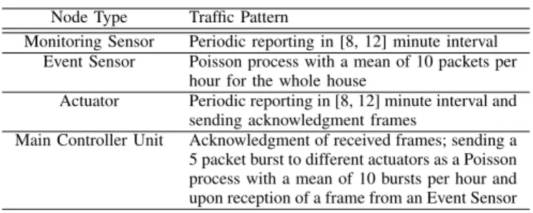
The traffic pattern of each node in the network depends on its assigned logical role. We have defined four logical types summarized in Table I. It is important to note that we have chosen the reporting periods and the general traffic patterns as suggested by IETF [10]. Nodes use UDP as the trans-port layer protocol and the application process acknowledges each received message. Therefore, traffic in the network is evenly distributed between point-to-multipoint and multipoint-to-point.
TABLE I
TRAFFIC PATTERN OF DIFFERENT NODE TYPES IN THE NETWORK. Node Type Traffic Pattern
Monitoring Sensor Periodic reporting in [8, 12] minute interval Event Sensor Poisson process with a mean of 10 packets per
hour for the whole house
Actuator Periodic reporting in [8, 12] minute interval and sending acknowledgment frames
Main Controller Unit Acknowledgment of received frames; sending a 5 packet burst to different actuators as a Poisson process with a mean of 10 bursts per hour and upon reception of a frame from an Event Sensor
C. Simulation Parameters
To closely reflect real deployments, nodes run Contiki OS with the whole protocol stack. We have compiled Contiki for the Tmote Sky platform based on MSP430 microcontroller with 10 KB of RAM and an IEEE 802.15.4 compliant radio [12]. By using the MSP430 hardware emulator, Cooja thus takes into account all the hardware constraints of the devices under study. Table II summarizes the Contiki OS and Cooja setups.
TABLE II
CONTIKIOSANDCOOJA PARAMETER SETUP.
Settings Value
Wireless channel model UDG Model with Distance Loss
Communication range 5 m
Mote type Tmote Sky
Transport and network layers UDP + µIPv6 + 6LoWPAN Max number of queued packets 2
MAC layer non-slotted CSMA + ContikiMAC Radio interface CC2420 2.4 GHz (IEEE 802.15.4)
Simulation time 8h
Notice a fairly low communication range at the PHY layer. Indeed, we have chosen this setup to reflect the assumption that nodes will operate with a very low power, i.e. with a low power amplifier gain mainly to reduce interference. Furthermore, radio-propagation obstacles present in a typical home environment, coupled with 2.4 GHz frequency, limit the communication range. With our parameters, the whole
house is covered within four hops as suggested before [10]. We have modified Contiki CSMA to buffer multicast packets and retransmit them when the channel was found busy at the initial attempt. Without this modification, the performance of LOADng was highly degraded due to a large number of dropped RREQ messages.
Another realistic assumption taken into account in our simulation was the use of ContikiMAC, a Radio Duty Cycling (RDC) protocol [13] based on preamble sampling and possibly sleeping receivers. Note that ContikiMAC operates on top of the IEEE 802.15.4 non-slotted CSMA and it may lead to some lost frames, which alleviates the assumption of the Unit Disk Graph that does not introduce any losses for nodes in the radio range.
TABLE III PROTOCOL PARAMETERS. (a) RPL
DIO Min Interval (s) 4 DIO Max Interval (s) 1048
Mode of Operation Storing
(b) LOADng Net Traversal Time (s) 10
Route Hold Time (s) 600, 1800,
RHT 3600
Table III summarizes RPL and LOADng protocol param-eters. Notice that we vary the Route Hold Time (RHT) of LOADng to study the protocol performance as a function of the route lifetime. RPL uses the Trickle algorithm [11] to emit DIO messages with default parameters and we have set the DIO Max Interval used in the steady state to approximately 17 minutes (1048 s). Tuning of RHT and the DIO Max Interval is an engineering challenge that should take into account the dynamic behavior of a given network, loss rate, and the probability of a node failure. Our choices for the LOADng parameters cover a broad range of cases. We can still decrease the overhead of RPL by increasing the DIO Max Interval.
We average the simulation results over 5 simulation runs and show 95 % confidence intervals. We plot CDF graphs using the cumulative results of 5 simulation runs.
V. PERFORMANCEEVALUATION
We first focus on a 25 node network (cf. Fig. 1) and evaluate LOADng and RPL in terms of packet delays, hop counts, and the routing table size. Furthermore, we study the control plane overhead and the average routing table size as a function of the number of nodes to show how the protocols scale for larger networks.
A. Packet Delay
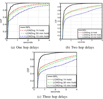
The latency studied in this section represents the total delay that a packet experiences from the instant it is passed to the UDP layer until it is successfully received at the destination. Fig. 2 presents the Cumulative Distribution Function (CDF) of packet delays for different hop counts. LOADng performs worse and packets experience significantly higher delays. Even though some LLNs can be delay insensitive, the interactive nature of home automation applications requires a routing protocol with delays of less than 0.5 seconds [10]. Due to the route discovery procedure of LOADng, the delay CDF con-verges slowly and 56.8 % of packets are within 0.5 seconds in
case of a 10 minute RHT. Flooding is less frequent when RHT increases to one hour and the delay becomes smaller. However, the delay CDF still converges slowly and approximately 26 % of packets experience a delay greater than 0.5 seconds (cf. Fig. 2a). The pro-active route discovery of RPL results in shorter delays and 90.9 % of packets experience a delay less than 0.5 seconds in case of the one hop distance.
0 1 2 3 4 0 0.2 0.4 0.6 0.8 1 seconds CDF RPL LOADng 1h hold LOADng 30 min hold LOADng 10 min hold
(a) One hop delays
0 1 2 3 4 0 0.1 0.2 0.3 0.4 0.5 0.6 0.7 0.8 0.9 1 seconds CD F RPL LOADng 1h hold LOADng 30 min hold LOADng 10 min hold
(b) Two hop delays
0 1 2 3 4 0 0.2 0.4 0.6 0.8 1 seconds CDF RPL LOADng 1h hold LOADng 30 min hold LOADng 10 min hold
(c) Three hop delays
Fig. 2. Packet delay CDFs in a 25 node network.
Packets going through one intermediate node, i.e. two hops away from the sink, (cf. Fig 2b) experience higher delay, as expected. In case of RPL, 15.4 % of packets experience a delay greater than 0.5 seconds. The maximal delay in this case is 2.4 seconds. With respect to the 1 hop distance delays, the delay CDF of RPL converges slightly slower due to the processing time and the channel contention at the intermediate node, because nodes have already a route. In case of LOADng and 1 hour RHT, 31 % of packets experience a delay greater than 0.5 sec.
Moving farther away from the sink does not significantly increase packet delays of RPL. However, we have observed a significant delay increase for LOADng. More precisely, 48.2 % of packets experience a delay greater than 0.5 seconds (cf. Fig. 2c). In case of a lower, 10 minute RHT, approximately 62 % of packets undergo a significant delay. The reason for the delay increasing with the hop distance is the flooding operation of LOADng as well as the instillation of forward routes. Basically, a node in the network sends a RREQ with the target address of the sink. Due to flooding, the sink receives more than one RREQ, each containing different path metrics. It responds with a RREP to the first RREQ and to all other RREQs with lower metrics. Nodes that form the reverse route and forward the RREPs towards its final destination instill the route towards the sink. The sink, however, does not have a route towards the intermediate nodes and upon the reception of a packet from them, has to flood the network with another RREQ before sending the acknowledgment. This results in
an increased delay with respect to packets destined to nodes physically closer to the sink.
B. Hop Distance
We have studied the optimality of the constructed routes through path hop and packet hop distances. The path hop distance represents the average number of hops between a source and a destination. As the traffic in the network is either multipoint-to-point or point-to-multipoint, the sink node is either a source or a destination of each packet. It is interesting to note that while RPL has built only bidirectional paths, some paths in LOADng networks are unidirectional, because of the stochastic nature of the flooding process. More precisely, most nodes add a route to the sink during the first sink-originated RREQ flooding. However, the reverse path is found at a later time, when the sink needs to address the node.
1 2 3 4 5 6 0 0.2 0.4 0.6 0.8 1 Number of Hops CDF RPL LOADng 1h hold LOADng 30 min hold LOADng 10 min hold
(a) CDF of path hop distances.
2 4 6 8 0 0.2 0.4 0.6 0.8 1 Number of Hops CDF RPL LOADng 1h hold LOADng 30 min hold LOADng 10 min hold
(b) CDF of packet hop distances. Fig. 3. Distance CDFs in the 25 node network.
Fig. 3a presents the CDF of path hop distances in the network. Notice that the RPL routes are shorter than those of LOADng. As mentioned in Section IV-A, the whole house is covered within four hops. The figure shows that the average path hop distances of RPL are bounded within four hops, which is not the case for LOADng. Moreover, 29 % of RPL routes are within one hop, while it is around 21 % for the LOADng, in the case of 10 minute RHT. This gap is even larger for two hop paths: 67 % of paths in case of RPL, while only 43 % in case of LOADng. Note that LOADng provides its most optimized routes in the case of a shorter RHT. There are two main reasons for this: i) due to the flooding operation the channel is saturated and some RREQ messages are dropped, because they reach the maximal number of attempts of the CSMA protocol, ii) as the nodes are memory constrained, they are only able to store two packets at a time, so RREQ messages that should be forwarded are often dropped. As a consequence, more frequent flooding (shorter RHT) supersedes the lost RREQs and gives more optimized routes.
Another issue is the following. If a node has a packet to send and the route is not ready, the most desired behavior, the one implemented in our case, is to buffer the packet. Once the RREP arrives, the node transmits the packet. However, the first arriving RREP is not necessarily the optimal one in terms of the route length. Therefore, the packet will follow a optimized route. We can notice in Fig. 3b that a non-negligible number of packets go over more than four hops. Upon reception of a subsequent RREP, the node will update its routing table and the following packets will follow the updated
route. On the other hand, routes constructed with RPL are optimal: not a single packet goes over more than 4 hops.
C. Routing Table Size
Due to the memory constraints of LLN devices, the routing table size is an important aspect. Fig. 4 shows the results for a 25 node network. 1 2 3 4 5 6 7 8 9 10 11 12 13 14 15 16 17 18 19 20 21 22 23 24 25 0 5 10 15 20 25 Av era ge Nu mb er of En trie si nt he Ro uti ng Ta ble Node ID RPL LOADng 1h hold LOADng 30 min hold LOADng 10 min hold
Fig. 4. Average number of routing table entries during the simulation. LOADng requires much higher number of entries with respect to RPL. Again, as a consequence of flooding, each node receiving a RREQ or on a route of a RREP, instills a route towards the sender, which results in a large number of unnecessary routes. Protocol implementors should thus care about the priority of RREP routes. This fact could endanger the operation of the protocol if a node runs out of the available memory. On the other hand, most nodes in the RPL network just have a default entry towards the preferred parent. However, depending on their position in the network, some nodes also have a significant number of entries. Namely, as the RPL operates in the storing mode, intermediate nodes selected as preferred parents by others, have to store downward routes. This is a critical issue, because if such a node runs out of memory, a loop may be formed.
15 20 25 30 35 40 0 5 10 15 20 25 Number of nodes Route Entries RPL
LOADng 10 min hold LOADng 30 min hold LOADng 1h hold
(a) Average number of route entries.
15 20 25 30 35 40 0 2 4 6 8 10 12 14x 10 6 Number of nodes bytes RPL
LOADng 10 min hold LOADng 30 min hold LOADng 1h hold
(b) Control plane overhead (bytes).
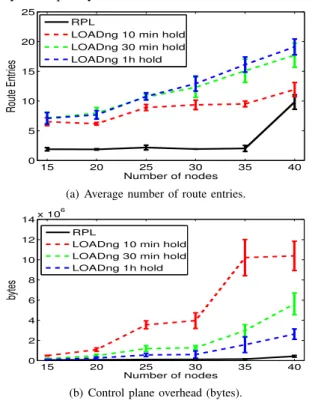
Fig. 5. Memory and overhead for an increased number of nodes.
To see how the protocols scale for a larger network, we have studied the average number of route entries as a function of an increasing number of nodes (cf. Fig. 5a). We can notice that the main consequence of having a long RHT is a significantly increasing number of route entries. With a shorter lifetime, the protocol scales better as the routes expire faster and the average number of required entries slowly increases. For RPL, the average number of routes slowly increases. However, it has a significantly higher number of entries for 40 nodes, a consequence of the limited number of neighbor entries that nodes can store. During the simulation time, we have observed oscillations in the RPL graph as parent nodes were constantly overwritten by other neighbors so that a number of nodes played the role of the preferred parent and stored downward routes. This behavior may impact the RPL operation for more dense networks.
D. Overhead
We have evaluated the routing overhead of the protocols as a function of an increasing number of nodes (cf. Fig. 5b presenting the overhead in bytes during the simulation time). Although the previous work [14] revealed a significantly higher overhead with RPL, our results show that RPL benefits from fairly low overhead compared to LOADng. We evaluate the total overhead as a sum of the lengths of all control messages passed from the routing protocols to the layers bellow. Note that by doing so, we avoid taking into account the overhead introduced by ContikiMAC.
We can notice that the implementation of ContikiRPL re-sults in a lower overhead than observed previously [14]. As the RPL RFC under-specifies the DAO control message emission, the overhead strongly depends on a given implementation. Fur-thermore, it is important to note that our simulation scenario does not trigger any global repairs of the RPL DODAG during the eight hours of simulation. In this way, our results give an idea about the performance of the two protocols in the steady state. Thus, we observe that most of the RPL overhead appears at the beginning of the simulation, reduced later by Trickle. The overhead of LOADng strongly depends on RHT: for a shorter RHT, nodes flood more frequently. We can notice from the figure that the total amount of the LOADng overhead sharply increases with the number of nodes due to the high density of nodes in the network, which may however, be reduced with an optimized flooding algorithm at the cost of a higher complexity.
The lifetime of battery-powered nodes directly relates to the use of the radio transceiver. More precisely, in case of the Tmote Sky platform, power consumption due to the radio use is three orders of magnitude larger than that due to CPU processing [12]. Thus, the control plane overhead and average number of hops of a protocol are the determining factors of the expected node lifetime. Our study shows that the control overhead of LOADng for short hold times does not scale well with dense deployments of smart home applications. As we expect an increasing number of devices in home networks, this effect may significantly impact the overall network lifetime.
VI. RELATEDWORK
Several authors analyzed the performance of RPL. An IETF draft [5] evaluates the protocol by considering several routing metrics in real-life deployment scenarios. Nuvolone studied stability delays of RPL using OmNet++ [15]. Clausen et al. studied the multipoint-to-point performance of RPL using NS2 [16]. The authors [17] evaluated different optimized broadcast techniques for the use in RPL [17]. Ko et al. presented the implementation of RPL for TinyOS and discussed its performance [6]. Ben Saad et al. used the Contiki framework to evaluate the performance of a PLC network serving as a LLN backbone [7]. Other authors studied the routing overhead and delay induced by ContikiRPL implementation [8]. Finally, an IETF draft [18] presented a thorough study of several critical issues in the RPL protocol.
Gomez et al. [19] compared various AODV-based routing protocols, including LOAD and discussed design tradeoffs. Iliev et al. [20] evaluated the route discovery delay as well as the round trip time induced by the TinyOS implementation of LOAD in real-life deployment scenarios.
Herberg et al. presented a comparative performance study of RPL and LOADng in case of bidirectional traffic using simulations in NS2 [14]. The paper shows a significantly larger control overhead of RPL caused by the maintenance of downward routes. It also compares the two protocols with an ideal routing protocol to show that RPL provides near-optimal routes while LOADng results in a certain gap. As the RPL RFC does not specify the period or the mechanism to use for maintaining downward routes, the study assumed an interval of 15 seconds. This choice is questionable, because it is the main cause of the high control overhead of RPL. Furthermore, the application-layer scenario used for the comparison is not the same for the two protocols. Thus, the question remains how LOADng and RPL perform under the same scenario.
VII. CONCLUSION
In the light of our study, RPL results in good overall per-formance for our Home Automation scenario while LOADng could serve better sparse LLN deployments with low-priority traffic in which the Route Hold Time can attain a large value. For Home Automation applications in which the response time is important, our results suggest that LOADng is not the best candidate. However, it is important to recall that we have used a simple flooding scheme and a better mechanism may reduce the control overhead. Furthermore, an intelligent route storing algorithm may reduce memory requirements of LOADng. These aspects are open research issues and their solutions will improve the efficiency and scalability, but at the cost of a higher implementation complexity.
We have confirmed the previous findings that RPL provides shorter routes and a smaller spanning tree depth compared to LOADng in our rather dense Home Automation topologies. We have also showed that RPL delays stay small and its overhead strongly depends on the implementation and a careful choice of parameters. Moreover, RPL has shown better results
and less memory requirements than LOADng, but at the price of a higher implementation complexity.
To sum up, several aspects remain interesting research challenges: reducing the specification complexity of RPL, optimizing flooding and route storage of LOADng as well as mixing the proactive and reactive approaches to maximize some performance criteria for a given application domain.
ACKNOWLEDGEMENTS
This work was partially supported by the European Com-mission project CALIPSO under contract 288879, the French National Research Agency (ANR) projects ARESA2 under contract ANR-09-VERS-017, and IRIS ANR-11-INFR-016. Many thanks to Chi-Anh La for making available the LOADng implementation.
REFERENCES
[1] G. Montenegro, N. Kushalnagar, and J. Hui, “Transmission of IPv6 packets over IEEE 802.15.4 networks,” IETF, RFC 4944, 2007. [2] T. Winter, P. Thubert, A. Brandt, T. Clausen, J. Hui, R. Kelsey, P. Levis,
K. Pister, R. Struik, and J. Vasseur, “RPL: IPv6 routing protocol for low power and lossy networks,” IETF, RFC 6550, April 2012.
[3] T. Clausen, A. C. de Verdiere, J. Yi, A. Niktash, Y. Igarashi, and U. Herberg, “The Lightweight On-demand Ad hoc Distance-vector Routing Protocol - Next Generation (LOADng),” IETF, Draft, Oct 2012. [4] C. Perkins, E. Belding-Royer, and S. Das, “Ad hoc On-Demand Distance
Vector (AODV) Routing,” IETF, RFC 3561, July 2003.
[5] A. Tripathi, J. de Oliveira, and J. Vasseur, “Performance evaluation of routing protocol for low power and lossy networks,” IETF, Draft, 2012. [6] J. Ko, S. Dawson-Haggerty, O. Gnawali, D. Culler, and A. Terzis, “Evaluating the performance of RPL and 6LoWPAN in TinyOS,” in
IPSN, 2011.
[7] L. Ben Saad, C. Chauvenet, and B. Tourancheau, “Simulation of the RPL Routing Protocol for IPv6 Sensor Networks: two cases studies,” in
SENSORCOMM. IARIA, Aug. 2011.
[8] N. Accettura, L. Grieco, G. Boggia, and P. Camarda, “Performance analysis of the RPL routing protocol,” in Mechatronics (ICM). IEEE, april 2011, pp. 767 –772.
[9] N. Tsiftes, J. Eriksson, N. Finne, F. ¨Osterlind, J. H¨oglund, and A. Dunkels, “A framework for low-power IPv6 routing simulation, experimentation, and evaluation,” SIGCOMM, vol. 40, no. 4, pp. 479– 480, 2010.
[10] A. Brandt, J. Buron, and G. Porcu, “Home Automation Routing Require-ments in Low-Power and Lossy Networks,” IETF, RFC 5826, 2010. [11] P. Levis, T. Clausen, J. Hui, O. Gnawali, and K. J, “The Trickle
Algorithm,” IETF, RFC 6206, 2011.
[12] Moteiv. Tmote Sky - ultra low power IEEE 802.15.4 compliant wireless sensor module. Datasheet.
[13] A. Dunkels, “The ContikiMAC radio duty cycling protocol,” Swedish Institute of Computer Science (SICS), Tech. Rep., 2011.
[14] U. Herberg and T. Clausen, “A comparative performance study of the routing protocols LOAD and RPL with bi-directional traffic in low-power and lossy networks,” in PE-WASUN. ACM, 2011, pp. 73–80. [15] M. Nuvolone, “Stability analysis of the delays of the routing protocol
over low power and lossy networks,” Master’s thesis, KTH RIT, 2010. [16] T. Clausen and U. Herberg, “Multipoint-to-point and broadcast in RPL,”
INRIA, Technical Report No. 7244, 2010.
[17] ——, “Comparative study of RPL-enabled optimized broadcast in wireless sensor networks,” in Intelligent Sensors, Sensor Networks and
Information Processing (ISSNIP), dec 2010, pp. 7 –12.
[18] T. Clausen, J. Yi, and U. Herberg, “Experiences with RPL: IPv6 routing protocol for low power and lossy networks,” IETF, Internet Draft, 2012. [19] C. Gomez, P. Salvatella, O. Alonso, and J. Paradells, “Adapting AODV for IEEE 802.15.4 mesh sensor networks: theoretical discussion and performance evaluation in a real environment,” in WoWMoM, 2006. [20] V. Iliev and J. Schoenwaelder, “Mesh routing for low-power mobile
ad-hoc wireless sensor networks using LOAD,” Jacobs University Bremen, Research Report, 2007.