HAL Id: lirmm-01362431
https://hal-lirmm.ccsd.cnrs.fr/lirmm-01362431
Submitted on 8 Sep 2016
HAL is a multi-disciplinary open access
archive for the deposit and dissemination of
sci-entific research documents, whether they are
pub-lished or not. The documents may come from
teaching and research institutions in France or
abroad, or from public or private research centers.
L’archive ouverte pluridisciplinaire HAL, est
destinée au dépôt et à la diffusion de documents
scientifiques de niveau recherche, publiés ou non,
émanant des établissements d’enseignement et de
recherche français ou étrangers, des laboratoires
publics ou privés.
SuMGra: Querying Multigraphs via Efficient Indexing
Vijay Ingalalli, Dino Ienco, Pascal Poncelet
To cite this version:
Vijay Ingalalli, Dino Ienco, Pascal Poncelet. SuMGra: Querying Multigraphs via Efficient
Index-ing. DEXA: Database and Expert Systems Applications, Sep 2016, Porto, Portugal. pp.387-401,
�10.1007/978-3-319-44403-1_24�. �lirmm-01362431�
SuMGra: Querying Multigraphs via Efficient
Indexing
Vijay Ingalalli1,2, Dino Ienco2, and Pascal Poncelet1
1Universit´e de Montpellier, LIRMM - Montpellier, France
E-mail: {pascal.poncelet,vijay}@lirmm.fr
2IRSTEA Montpellier, UMR TETIS
F-34093 Montpellier, France E-mail: [email protected]
Abstract. Many real world datasets can be represented by a network with a set of nodes interconnected with each other by multiple relations. Such a rich graph is called a multigraph. Unfortunately, all the exist-ing algorithms for subgraph query matchexist-ing are not able to adequately leverage multiple relationships that exist between the nodes. In this paper we propose an efficient indexing schema for querying single large multi-graphs, where the indexing schema aptly captures the neighbourhood structure in the data graph. Our proposal SuMGra couples this novel indexing schema with a subgraph search algorithm to quickly traverse though the solution space to enumerate all the matchings. Extensive ex-periments conducted on real benchmarks prove the time efficiency as well as the scalability of SuMGra .
1
Introduction
Many real world datasets can be represented by a network with a set of nodes interconnected with each other by multiple relations. Such a rich graph is called multigraph and it allows different types of edges in order to represent different types of relations between vertices [1, 2]. Example of multigraphs are: social networks spanning over the same set of people, but with different life aspects (e.g. social relationships such as Facebook, Twitter, LinkedIn, etc.); protein-protein interaction multigraphs created considering the pairs of protein-proteins that have direct interaction/physical association or they are co-localised [15]; gene multigraphs, where genes are connected by considering the different pathway interactions belonging to different pathways; RDF knowledge graph where the same subject/object node pair is connected by different predicates [10].
One of the difficult operation in graph data management is subgraph query-ing [6]. Although subgraph queryquery-ing is an NP-complete [6] problem, practically, we can find embeddings in real graph data by employing a good matching order and intelligent pruning rules. In literature, different families of subgraph match-ing algorithms exist. A first group of techniques employ Feature based indexmatch-ing
followed by a filtering and verification framework. During filtering, some graph patterns (subtrees or paths) are chosen as indexing features to minimize the number of candidate graphs. Then the verification step checks for the subgraph isomorphism using the selected candidates [14, 4, 16, 11]. All these methods are developed for transactional graphs, i.e. the database is composed of a collection of graphs and each graph can be seen as a transaction of such database, and they cannot be trivially extended on the single multigraph scenario. A second family of approaches avoids indexing and it uses Backtracking algorithms to find embeddings by growing the partial solutions. In the beginning, they obtain a potential set of candidate vertices for every vertex in the query graph. Then a recursive subroutine called SubgraphSearch is invoked to find all the possible embeddings of the query graph in the data graph [5, 13, 7]. All these approaches are able to manage graphs with only a single label on the vertex. Although in-dex based approaches focus on transactional database graphs, some backtrack-ing algorithms address the large sbacktrack-ingle graph settbacktrack-ing [9]. All these methods are not conceived to manage and query multigraphs and their extension to manage multiple relations between nodes cannot be trivial. A third and recent family of techniques defines equivalence classes at query and/or database level, by ex-ploiting vertex relationships. Once the data vertices are grouped into equivalence classes, the search space is reduced and the whole process is speeded up [6, 12]. Adapting these methods to multigraph is not straightforward since, the differ-ent types of relationships between vertices can expondiffer-entially increase the number of equivalent classes (for both query and data graph) thereby drastically reduc-ing the efficiency of these strategies. Among the vast literature on subgraph isomorphism, [3] is the unique approach, which is a backtracking approach, that is able to directly manage graph with (multiple) labels on the edges. It proposes an approach called RI that uses light pruning rules in order to avoid visiting useless candidates.
Due to the availability of multigraph data and the importance of performing query on multigraph data, in this paper, we propose a novel method SuMGra that supports subgraph matching in a multigraph via efficient indexing. In par-ticular, we capture the multigraph properties in order to build the index struc-tures, and we show that by exploiting multigraph properties, we are able to perform subgraph matching very efficiently. As observed in Table 1, the pro-posed SuMGra is almost one order of magnitude better than the benchmark approach RI, for the DBPEDIA dataset and for the query sizes from 3 to 11.
Approach 3 5 7 9 11
SuMGra 160.5 254.1 545.7 971.5 1610.9 RI 7045.7 7940.8 7772.7 6872.6 8502.5
Table 1. Time (msec) taken by RI and SuMGra for DBPEDIA dataset Deviating from all the previous proposed approaches, we conceive an index-ing schema to summarize information contained in a sindex-ingle large multigraph. SuMGra involves two main phases: (i) an off-line phase that builds efficient indexes for the information contained in the multigraph; (ii) an on-line phase, where a search procedure exploits the indexing schema previously built. The
rest of the paper is organized as follows. Background and problem definition are provided in Section 2. An overview of the proposed approach is presented in Section 3, while Section 4 and Section 5 describe the indexing schema and the query subgraph search algorithm, respectively. Section 6 presents experimental results. Conclusions are drawn in Section 7.
2
Preliminaries and Problem Definition
Formally, we can define a multigraph G as a tuple of four elements (V, E, LE, D) where V is the set of vertices and D is the set of dimensions , E ⊆ V × V is the
set of undirected edges and LE : V × V → 2Dis a labelling function that assigns
the subset of dimensions to each edge it belongs to. In this paper, we address the sub-graph isomorphism problem for undirected multigraphs.
Definition 1 Subgraph isomorphism for undirected multigraph. Given a
multi-graph Q = (Vq, Eq, LqE, Dq) and a multigraph G = (V, E, LE, D), the subgraph
isomorphism from Q to G is an injective function ψ : Vq → V such that:
∀(um, un) ∈ Eq, ∃ (ψ(um), ψ(un)) ∈ E and L
q
E(um, un) ⊆ LE(ψ(um), ψ(un)).
Problem Definition. Given a query multigraph Q and a data multigraph G, the subgraph query problem is to enumerate all the embeddings of Q in G.
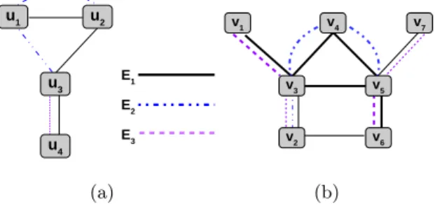
For the ease of representation, in the rest of the paper, we simply refer to a data multigraph G as a graph, and a query multigraph Q as a subgraph. We also enumerate (for unique identification) the set of query vertices by U and the set of data vertices by V . E1 E2 E3 u1 u2 u3 u4 (a) v1 v4 v7 v3 v5 v6 v2 (b)
Fig. 1. A sample (a) query multigraph Q and (b) data multigraph G
In Figure 1, we introduce a query multigraph Q and a data multigraph G. The two valid embeddings for the subgraph Q are marked by the thick lines in the
graph G and are enumerated as follows: R1:= {[u1, v4], [u2, v5], [u3, v3], [u4, v1]};
R2:= {[u1, v4], [u2, v3], [u3, v5], [u4, v6]}; where, each query vertex ui is matched
to a distinct data vertex vj, written as [ui, vj].
3
An Overview of SuMGra
In this section, we sketch the main idea behind our proposal. The entire proce-dure can be divided into two parts: (i) an indexing schema for the graph G that
exploits edge dimensions and the vertex neighbourhood structure (Section 4) (ii) a subgraph search algorithm, that integrates recent advances in the graph data management field, to enumerate the embeddings of the subgraph (Section 5).
The overall idea of SuMGra is depicted in Algorithm 1. Initially, we order the set of query vertices U using a heuristic proposed in Section 5.1. With an
or-dered set of query vertices Uo, we use the indexing schema to find a list of possible
candidate matches only for the initial query vertex uinitby calling SelectCand
(Line 5), as described in Section 5.2. Then, for each possible candidate of the initial query vertex, we call the recursive subroutine SubgraphSearch, that performs the subgraph isomorphism test.
The SubgraphSearch procedure (Section 5.3), finds the embeddings
start-ing with the possible matches for the initial query vertex uinit(Lines 7-11). Since
uinit has |Cuinit| possible matches, SubgraphSearch iterates through |Cuinit|
solution trees in a depth first manner until an embedding is found. That is, Sub-graphSearch is recursively called to find the matchings that correspond to all
ordered query vertices Uo. The partial embedding is stored in M = [M
q, Mg]
- a pair that contains the already matched query vertices Mq and the already
matched data vertices Mg. Once the partial embedding grows to become a
com-plete embedding, the repository of embeddings R is updated. Algorithm 1: SuMGra
1 Input: subgraph Q, graph G, indexes S, N
2 Output: R: all the embeddings of Q in G
3 Uo= OrderQueryVertices(Q, G)
4 uinit= u|u ∈ Uo
5 Cuinit = SelectCand(uinit, S)
6 R = ∅ /* Embeddings of Q in G */
7 for each vinit∈ Cu initdo
8 Mq= uinit; /* Matched initial query vertex */
9 Md= vinit; /* Matched possible data vertex */
10 M = [Mq, Mg] /* Partial matching of Q in G */
11 Update: R := SubgraphsSearch(R, M, N , Q, G, Uo)
12 return R
4
Indexing
In this section, we propose the indexing structures that are built on the data multigraph G, by leveraging the multigraph properties in specific; this index is used during the subgraph querying procedure. The primary goal of indexing is to make the query processing time efficient. For a lucid understanding of our indexing schema, we introduce a few definitions.
Definition 2 Vertex signature. For a vertex v, the vertex signature σ(v) is a multiset containing all the multiedges that are incident on v, where a multiedge
between v and a neighbouring vertex v0 is represented by a set that corresponds
to edge dimensions. Formally, σ(v) =S
v0∈N (v)LE(v, v0) where N (v) is the set
of neighbourhood vertices of v, and ∪ is the union operator for multiset. For instance, in Figure 1(b), σ(v6) = {{E1, E3}, {E1}}. The vertex signature is an intermediary representation that is exploited by our indexing schema.
The goal of constructing indexing structures is to find the possible candidate set for the set of query vertices u, thereby reducing the search space for the SubgraphSearch procedure, making SuMGra time efficient.
Definition 3 Candidate set. For a query vertex u, the candidate set C(u) is defined as C(u) = {v ∈ g|σ(u) ⊆ σ(v)}.
In this light, we propose two indexing structures that are built offline: (i) given the vertex signature of all the vertices of graph G, we construct a vertex signature index S by exploring a set of features f of the signature σ(v) (ii) we build a vertex neighbourhood index N for every vertex in the graph G. The index S is used to select possible candidates for the initial query vertex in the Select-Cand procedure while the index N is used to choose the possible candidates for the rest of the query vertices during the SubgraphSearch procedure.
4.1 Vertex Signature Index S
This index is constructed to enumerate the possible candidate set only for the initial query vertex. Since we cannot exploit any structural information for the initial query vertex, S captures the edge dimension information from the data vertices, so that the non suitable candidates can be pruned away.
We construct the index S by organizing the information supplied by the vertex signature of the graph; i.e., observing the vertex signature of data vertices, we intend to extract some interesting features. For example, the vertex signature
of v6, σ(v6) = {{E1, E3}, {E1}} has two sets of dimensions in it and hence v6 is
eligible to be matched with query vertices that have at most two sets of items
in their signature. Also, σ(v2) = {{E2, E3, E1}, {E1}} has the edge dimension
set of maximum size 3 and hence a query vertex must have the edge dimension set size of at most 3. More such features (e.g., the number of unique dimensions, the total number of occurrences of dimensions, etc.) can be proposed to filter out irrelevant candidate vertices. In particular, for each vertex v, we propose to extract a set of characteristics summarizing useful features of the neighbourhood of a vertex. Those features constitute a synopses representation (surrogate) of the original vertex signature.
In this light, we propose six |f |= 6 features, that leverage the multigraph properties; the features will be illustrated with the help of the vertex signature σ(v3) = {{E1, E2, E3}, {E1, E3}, {E1, E2}, {E1}}:
f1 Cardinality of vertex signature, (f1(v3) = 4)
f2 The number of unique dimensions in the vertex signature, (f2(v3) = 3)
f3 The number of all occurrences of the dimensions (repetition allowed), (f3(v3) = 8)
f4 Minimum index of the lexicographically ordered edge dimensions, (f4(v3) = 1)
f5 Maximum index of the lexicographically ordered edge dimensions, (f5(v3) = 3)
f6 Maximum cardinality of the vertex sub-signature, (f6(v3) = 3)
By exploiting the aforementioned features, we build the synopses to repre-sent the vertices in an efficient manner that will help us to select the eligible candidates during query processing.
Once the synopsis representation for each data vertex is computed, we store the synopses in an efficient data structure. Since each vertex is represented by a synopsis of several fields, a data structure that helps in efficiently performing range search for multiple elements would be an ideal choice. For this reason, we build a |f |-dimensional R-tree, whose nodes are the synopses having |f | fields.
The general idea of using an R-tree structure is as follows: A synopses
F = {f1, . . . , f|f |} of a data vertex spans an axesparallel rectangle in an f
-dimensional space, where the maximum co-ordinates of the rectangle are the
values of the synopses fields (f1, . . . , f|f |), and the minimum co-ordinates are
the origin of the rectangle (filled with zero values). For example, a data vertex
represented by the synopses with two features Fv= (2, 3) spans a rectangle in a
2-dimensional space in the interval range ([0, 2], [0, 3]). Now if we consider
syn-opses of two query vertices, Fu1 = (1, 3) and Fu2 = (1, 4), we observe that the
rectangle spanned by Fu1is wholly contained in the rectangle spanned by Fvbut
Fu2 is not wholly contained in Fv. Formally, the possible candidates for vertex
u can be written as P(u) = {v|∀i∈[1,...,f ]Fu(i) ≤ Fv(i)}, where the constraints
are met for all the |f |-dimensions. Since we apply the same inequality constraint
to all the fields, we need to pre-process few synopses fields; e.g., the field f4
contains the minimum value of the index, and hence we negate f4 so that the
rectangular containment problem still holds good. Thus, we keep on inserting the synopses representations of each data vertex v into the R-tree and build the index S, where each synopses is treated as an |f |-dimensional node of the R-tree.
4.2 Vertex Neighbourhood Index N
The aim of this indexing structure is to find the possible candidates for the rest of the query vertices.
Since the previous indexing schema enables us to select the possible candi-date set for the initial query vertex, we propose an index structure to obtain the possible candidate set for the subsequent query vertices. The index N will help us to find the possible candidate set for a query vertex u during the Subgraph-Search procedure by retaining the structural connectivity with the previously matched candidate vertices, while discovering the embeddings of the subgraph Q in the graph G.
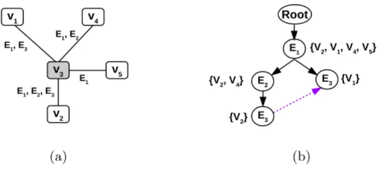
The index N comprises of neighbourhood trees built for each of the data vertex v. To understand the index structure, let us consider the data vertex v3 from Figure 1(b), shown separately in Figure 2(a). For this vertex v3, we collect all the neighbourhood information (vertices and multiedges), and represent this information by a tree structure. Thus, the tree representation of a vertex v con-tains the neighbourhood vertices and their corresponding multiedges, as shown in Figure 2(b), where the nodes of the tree structure are represented by the edge dimensions.
In order to construct an efficient tree structure, we propose the structure
- Ordered Trie with Inverted List (OTIL). Consider a data vertex vi, with a
set of n neighbourhood vertices N (vi). Now, for every pair (vi, Nj(vi)), where
which is inserted into the OTIL structure. Each multiedge is ordered (with the increasing edge dimensions), before inserting into OTIL structure, and the order is universally maintained for both query and data vertices. Further, for every
edge dimension Ei that is inserted into the OTIL, we maintain an inverted list
that contains all the neighbourhood vertices N (vi), that have the edge dimension
Ei incident on them. For example, as shown in Figure 2(b), the edge E2 will
contain the list {v2, v4}, since E2forms an edge between v3and both v2and v4.
To construct the OTIL index as shown in Figure 2(b), we insert each ordered multiedge that is incident on v at the root of the trie structure. To make index querying more time efficient, the OTIL nodes with identical edge dimension (e.g., E3) are internally connected and thus form a linked list of data vertices. For example, if we want to query the index in Figure 2(b) with a vertex having edges {E1, E3}, we do not need to traverse the entire OTIL. Instead, we perform a pre-ordered search, and as soon as we find the first set of matches, which is {V2}, we will be redirected to the OTIL node, where we can fetch the matched
vertices much faster (in this case {V1}), thereby outputting the set of matches
as {V2, V1}. E1, E3 v1 v4 v3 v5 v2 E1, E2, E3 E1, E2 E1 (a) E1 {V2, V1, V4, V5} Root E2 E3 E3 {V1} {V2} {V2, V4} (b)
Fig. 2. (a) Neighbourhood structure of v3 and (b) Neighbourhood Index for vertex v3
5
Subgraph Query Processing
We now proceed with the subgraph query processing. In order to find the em-beddings of a subgraph, we not only need to find the valid candidates for each query vertex, but also retain the structure of the subgraph to be matched.
5.1 Query Vertex Ordering
Before performing query processing, we order the set of query vertices U into
an ordered set of query vertices Uo. It is argued that an effective ordering of
the query vertices improves the efficiency of subgraph querying [9]. In order to achieve this, we propose a heuristic that employs two scoring functions.
The first scoring function relies on the number of multiedges of a query vertex. For each query vertex ui, the number of multiedges incident on it is
assigned as a score; i.e., r1(ui) = Pm
j=1|σ(u
j
i)|, where ui has m multiedges,
|σ(uji)| captures the number of edge dimensions in the jth multiedge. Query
vertices are ordered in ascending order considering the scoring function r1, and
thus uinit = argmax(r1(ui)). For example, in Figure 1(a), vertex u3 has the
maximum number of edges incident on it, which is 4, and hence is chosen as an initial vertex.
The second scoring function depends on the structure of the subgraph. We
maintain an ordered set of query vertices Uo and keep adding the next eligible
query vertex. In the beginning, only the initial query vertex uinit is in Uo.
The set of next eligible query vertices Unbro are the vertices that are in the
1-neighbourhood of Uo. For each of the next eligible query vertex u
n ∈ Unbro ,
we assign a score depending on a second scoring function defined as r2(un) =
|{Uo∩ adj(un)}|. It considers the number of the adjacent vertices of u
n that are
present in the already ordered query vertices Uo.
Then, among the set of next eligible query vertices Uo
nbr for the already
or-dered Uo, we give first priority to function r2and the second priority to function
r1. Thus, in case of any tie ups, w.r.t. r2, the score of r1 will be considered.
When both r2and r1leave us in a tie up situation, we break such tie at random.
5.2 Select Candidates for Initial Query Vertex
For the initial query vertex uinit, we exploit the index structure S to retrieve the set of possible candidate data vertices, thereby pruning the unwanted candidates for the reduction of search space.
During the SelectCand procedure (Algorithm 1, Line 5), we retrieve the possible candidate vertices from the data graph by exploiting the vertex signa-ture index S. However, since querying S would not prune away all the unwanted
vertices for uinit, the corresponding partial embeddings would be discarded
dur-ing the SubgraphSearch procedure. For instance, to find candidate vertices
for uinit = u3, we build the synopses for u3 and find the matchable vertices in
G using the index S. As we recall, synopses representation of each data vertex spans a rectangle in the d-dimensional space. Thus, it remains to check, if the
rectangle spanned by u3 is contained in any of rectangles spanned by the
syn-opses of the data vertices, with the help of R-tree built on data vertices, which results in the candidate set {v3, v5}.
5.3 Subgraph Searching
The SubgraphSearch recursive procedure is described in Algorithm 2. Once an
initial query vertex uinitand its possible data vertex vinit∈ Cuinit, that could be
a potential match, is chosen from the set of select candidates, we have the partial
solution pair M = [Mq, Mg] of the subgraph query pattern we want to grow. If
vinit is a right match for uinit, and we succeed in finding the subsequent valid
matches for Uo, we will obtain an embedding; else, the recursion would revert
Algorithm 2: SubgraphSearch(R, M, N , Q, G, Uo)
1 Fetch unxt∈ Uo /* Fetch query vertex to be matched */
2 MC = FindJoinable(Mq, Mg, N , unxt) /* Matchable candidate vertices */
3 if |MC|6= ∅ then
4 for each vnxt∈ MCdo
5 Mq= Mq∪ unxt;
6 Mg= Mg∪ vnxt;
7 M = [Mq, Mg] /* Partial matching grows */
8 SubgraphSearch(R, M, N , Q, G, Uo)
9 if (|M | == |Uo|) then
10 R = R ∪ M /* Embedding found */
11 return R
In the beginning of SubgraphSearch procedure, we fetch the next query
vertex unxtfrom the set of ordered query vertices Uo, that is to be matched (Line
1). Then FindJoinable procedure finds all the valid data vertices that can be
matched with the next query vertex unxt (Line 2). The main task of subgraph
matching is done by the FindJoinable procedure, depicted in Algorithm 3.
Once all the valid matches for unxt are obtained, we update the solution pair
M = [Mq, Mg] (Line 5-7). Then we recursively call SubgraphSearch procedure
until all the vertices in Uo have been matched (Line 8). If we succeed in finding
matches for the entire set of query vertices Uo, then we update the repository
of embeddings (Line 9-10); else, we keep on looking for matches recursively in the search space, until there are no possible candidates to be matched for unxt (Line 3).
Algorithm 3: FindJoinable(Mq, Mg, N , unxt)
1 Aq:= Mq∩ adj(unxt) /* Matched query neighbours */
2 Ag:= {v|v ∈ Mg} /* Corresponding matched data neighbours */
3 Intialize: MCtemp= 0, MC= 0
4 MCtemp= ∩|Aq |i=1 NeighIndexQuery(N , Aig, (A i q, unxt))
5 for each vc∈ MCtempdo
6 if σ(vc) ⊇ σ(unxt) then
7 add vcto MC /* A valid matchable vertex */
8 return MC
The FindJoinable procedure guarantees the structural connectivity of the embeddings that are outputted. Referring to Figure 1, let us assume that the
already matched query vertices Mq = {u2, u3} and the corresponding matched
data vertices Mg= {v3, v5}, and the next query vertex to be matched unxt= u1.
Initially, in the FindJoinable procedure, for the next query vertex unxt, we
collect all the neighbourhood vertices that have been already matched, and store
them in Aq; formally, Aq := Mq∩ adj(unxt) and also collect the corresponding
matched data vertices Ag(Line 1-2). For instance, for the next query vertex u1,
Now we exploit the neighbourhood index N in order to find the valid matches
for the next query vertex unxt. With the help of vertex N , we find the possible
candidate vertices MCtemp for each of the matched query neighbours Ai
q and the
corresponding matched data neighbour Aig.
To perform querying on the index structure N , we fetch the multiedge that
connects the next matchable query vertex unxt and the ith previously matched
query vertex Ai
q. We now take the multiedge (Aiq, unxt) and query the index
structure N of the correspondingly matched data vertex Ai
g (Line 4). For
in-stance, with Ai
q = u2, and unxt= u1 we have a multiedge {E1, E2}. As we can
recall, each data vertex vj has its neighbourhood index structure N (vj),
repre-sented by an OTIL structure. The elements that are added to OTIL are nothing but the multiedges that are incident on the vertex vj, and hence the nodes in the tree are nothing but the edge dimensions. Further, each of these edge dimensions
(nodes) maintain a list of neighbourhood (adjacent) data vertices of vj that
con-tain the particular edge dimension as depicted in Figure 2(b). Now, when we look
up for the multiedge (Aiq, unxt), which is nothing but a set of edge dimensions, in
the OTIL structure N (Ai
g), two possibilities exist. (1) The multiedge (Aiq, unxt)
has no matches in N (Aig) and hence, there are no matchable data vertices for the
next query vertex unxt. (2) The multiedge (Aiq, unxt) has matches in N (Aig) and
hence, NeighIndexQuery returns a set of possible candidate vertices MCtemp.
The set of vertices MCtemp, present in the OTIL structure as a linked list, are the
possible data vertices since, these are the neighbourhood vertices of the already
matched data vertex Ai
g, and hence the structure is maintained. For instance,
multiedge {E1, E2} has a set of matched vertices {v2, v4} as we can observe in
Figure 2(a).
Further, we check if the next possible data vertices are maintaining the
struc-tural connectivity with all the matched data neighbours Ag, that correspond to
matched query vertices Aq, and hence we collect only those possible candidate
vertices MCtemp, that are common to all the matched data neighbours with the
help of intersection operation ∩. Thus we repeat the process for all the matched
query vertices Aq and the corresponding matched data vertices Ag to ensure
structural connectivity (Line 4). For instance, with A1
q = u2 and corresponding
A1
g= v3, we have M
temp
C 1= {v2, v4}; with A2q = u3 and corresponding A2g= v5,
we have MCtemp2= {v4}, since the multiedge between (Ai
q, unxt) is {E2}. Thus,
the common vertex v4is the one that maintains the structural connectivity, and
hence belongs to the set of matchable candidate vertices MCtemp= v4.
The set of matchable candidates MCtempare the valid candidates for unxtboth
in terms of edge dimension matching and the structural connectivity with the already matched partial solution. However, at this point, we propose a strategy that predicts whether the further growth of the partial matching is possible, w.r.t. to the neighbourhood of already matched data vertices, thereby pruning the search space. We can do this by checking the condition whether the vertex
signature σ(unxt) is contained in the vertex signature of v ∈ MCtemp(Line 11-13).
about the unmatched query vertices that are in the neighbourhood of already
matched data vertices. For instance, v4 can be qualified as MC since σ(v4) ⊇
σ(u1). That is, considering the fact that we have found a match for u1, which
is v4, and that the next possible query vertex is u4, the superset containment check will assure us the connectivity (in terms of edge dimensions) with the next possible query vertex u4. Suppose a possible candidate data vertex fails this superset containment test, it means that, the data vertex will be discarded by FindJoinable procedure in the next iteration, and we are avoiding this useless step in advance, thereby making the search more time efficient.
In order to efficiently address the superset containment problem between the
vertex signatures σ(vc) and σ(unxt), we model this task as a maximum matching
problem on a bipartite graph [8]. Basically, we build a bipartite graph whose nodes are the sub-signatures of σ(vc) and σ(unxt); and an edge exists between a pair of nodes only if the corresponding sub-signatures do not belong to the
same signature, and the ithsub-signature of vc is a superset of jthsub-signature
of unxt. This construction ensures to obtain at the end a bipartite graph. Once the bipartite graph is built we run a maximum matching algorithm to find a maximum match between the two signatures. If the size of the maximum match found is equal to the size of σ(unxt), the superset operation returns true otherwise σ(unxt) is not contained in the signature σ(vc). To solve the maximum matching problem on the bipartite graph, we employ the Hopcroft-Karp [8] algorithm.
6
Experimental Evaluation
In this section, we evaluate the performance of SuMGra on real multigraphs. We evaluate the performance of SuMGra by comparing it with two base-line approaches (its own variants) and a competitor RI [3]. The two basebase-line approaches are: (i) SuMGra-No-SC that does not consider the vertex
signa-ture index S and it initializes the candidate set of the initial vertex C(uinit)
with the whole set of data nodes; (ii) SuMGra-Rand-Order that consider all the indexing structure but it employs a random ordering of the query vertices preserving connectivity. The RI approach is able to manage graphs with multi-edges, and we obtain the implementation from the original authors. For the purpose of evaluation. we consider three real world multigraphs: DBLP data set
built by following the procedure adopted in [1]; FLICKR 1crawled from Flickr,
which is an image and video hosting website, web services suite, and an online
community; DBPEDIA 2 that is the well-known knowledge base built by the
Semantic Web Community. For DBLP, vertices correspond to different authors and each dimensions represent one of the top 50 Computer Science conferences. Two authors are connected over a dimension if they co-authored at least one paper together in that conference. In FLICKR, users are represented by nodes, and blogger’s friends are represented using edges. Multiple edges exist between two users if they have common multiple memberships. The RDF format in which
1
http://socialcomputing.asu.edu/pages/datasets
2
DBPEDIA is stored can naturally be modeled as a multigraph where vertices are subjects and objects of the RDF triplets and edges represent the predicates between them. Benchmark characteristics are reported in Table 2.
To test the behavior of the different approaches, we generate random queries [7, 13] varying their size (in terms of vertices) from 3 to 11 in steps of 2. All the generated queries contain one (or more) edge with at least two dimensions. In order to generate queries that can have at least one embedding, we sample them from the corresponding multigraph. For each dataset and query size we obtain 1 000 samples. Following the methodology previously proposed [6, 11], we report the average time values considering the first 1 000 embeddings for each query. It should be noted that the queries returning no answers were not counted in the statistics (the same statistical strategy has been used by [7, 11]).
All the experiments were run on a server, with 64-bit Intel 6 processors @ 2.60GHz, and 250GB RAM, running on a Linux OS - Ubuntu. Our methods have been implemented using C++.
Dataset Nodes Edges Dim Density
DBLP 83 901 141 471 50 4.0e-5
FLICKR 80 513 5 899 882 195 1.8e-3 DBPEDIA 4 495 642 14 721 395 676 1.4e-6
Table 2. Benchmark statistics.
Dataset S N
DBLP 1.15 0.37
FLICKR 1.55 8.89 DBPEDIA 64.51 66.59 Table 3. Index Construction Time (secs.).
6.1 Performance of SuMGra
Table 3 reports the index construction time of SuMGra for each of the employed dataset. As we can observe for the bigger datasets like FLICKR, and DBPEDIA, construction of the index N takes more time when compared to the construction of S. This happens due to either huge number of edges, or nodes or both in these two datasets. For DBLP we can observe the opposite phenomenon. This can be explained by the small number of edges and dimensions present in this dataset. Among all the datasets, DBPEDIA is the most expensive dataset in terms of indices construction but it always remains reasonable as time consumption for the off-line step is around one minute for each index.
Query Processing Time Figures 3, 4 and 5 summarize time results. All the times we report are in milliseconds; the Y-axis (logarithmic in scale) represents the query matching time; the X-axis represents the increasing query sizes.
We also analyse the time performance of SuMGra by varying the number of edge dimensions in the subgraph. In particular, we perform experiments for query multigraphs with two different edge dimensions: d = 2 and d = 4. That is, a query with d = 2 has at least one edge that exists in at least 2 dimensions. The same analogy applies to the queries with d = 4.
For DBLP dataset, we observe in Figure 3 that SuMGra performs the best in all the situations, and in fact it outperforms the other approaches by
100 101 102 103
3 4 5 6 7 8 9 10 11
Avg. elapsed time (msec.)
Query Size (# of vertices) RI SumGra-No-SC SumGra-Rand-Order SumGra (a) 10-1 100 101 102 103 3 4 5 6 7 8 9 10 11
Avg. elapsed time (msec.)
Query Size (# of vertices) RI
SumGra-No-SC
SumGra-Rand-Order SumGra
(b)
Fig. 3. Query Time on DBLP dataset for (a) with d = 2 (b) with d = 4
100 101 102 103 104 3 4 5 6 7 8 9 10 11
Avg. elapsed time (msec.)
Query Size (# of vertices) RI SumGra-No-SC SumGra-Rand-Order SumGra (a) 100 101 102 103 104 3 4 5 6 7 8 9 10 11
Avg. elapsed time (msec.)
Query Size (# of vertices) RI
SumGra-No-SC
SumGra-Rand-Order SumGra
(b)
Fig. 4. Query Time on FLICKR dataset for (a) with d = 2 (b) with d = 4
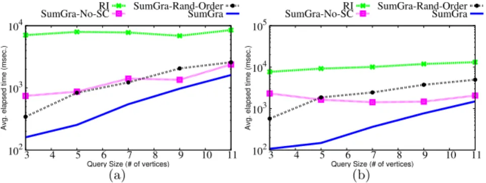
102 103 104
3 4 5 6 7 8 9 10 11
Avg. elapsed time (msec.)
Query Size (# of vertices) RI
SumGra-No-SC SumGra-Rand-OrderSumGra
(a) 102 103 104 105 3 4 5 6 7 8 9 10 11
Avg. elapsed time (msec.)
Query Size (# of vertices) RI
SumGra-No-SC SumGra-Rand-OrderSumGra
(b)
Fig. 5. Query Time on DBPEDIA dataset (a) for d = 2 (b) d = 4
a huge margin. This happens thanks to both: a rigorous pruning of candidate vertices for initial query vertex as underlined by the gain w.r.t. SuMGra-No-SC and an efficient query vertex ordering strategy as highlighted by the difference w.r.t. SuMGra-Rand-Order. For the FLICKR dataset (Figure 4) SuMGra, SuMGra-No-SC and SuMGra-Rand-Order outperform RI. For many query
instances, especially for FLICKR, SuMGra-No-SC obtains better performance than RI while SuMGra still outperforms competitors. We can observe that random query ordering drastically affects the performance pointing out the im-portance of this step. Moving to DBPEDIA dataset in Figure 5, we observe a significant deviation between RI and SuMGra, with SuMGra winning by a huge margin.
To conclude, we note that SuMGra outperforms the considered competitors, for all the employed benchmarks for all query size. Its performance is reported as best for multigraphs having many edge dimensions - FLICKR and high spar-sity - DBPEDIA. Thus, we highlight that SuMGra is robust in terms of time performance varying both the query size and dimensions.
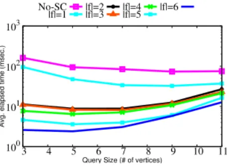
Assessing the Set of Synopses Features In this experiment we assess the quality of the features composing the synopses representation for our indexing schema. To this end, we vary the features we consider to build the synopsis representation to understand if some of them can be redundant and/or do not improve the final performance. Since visualizing the combination of the whole set of features will be hard, we limit this experiment to a subset of combinations. Hence, we choose to vary the size of the feature set from one to six, by considering the order defined in Section 4.1. Using all the six features results in the proposed approach SuMGra. 100 101 102 103 3 4 5 6 7 8 9 10 11
Avg. elapsed time (msec.)
Query Size (# of vertices) No-SC
|f|=1 |f|=2|f|=3 |f|=4|f|=5 |f|=6
Fig. 6. Query time with varying syn-opses fields for DBLP with d = 4
We perform experiments with different con-figurations that have varying number of syn-opses features; for instance |f |= 3| means that it considers only first three features to build synopses. Although we report plots only for DBLP for queries with d = 4, the behaviour for different datasets has similar behaviour. Results are reported in Figure 6. We note that, considering the entire set of features drasti-cally improves the time performance, when compared to a subset of these six features. We conclude that the different features are not re-dundant and they are all helpful in pruning the useless data vertices.
7
Conclusion
We proposed an efficient strategy to support Subgraph Matching in a Multi-graph via efficient indexing. The proposed indexing schema leverages the rich structure available in the multigraph. The different indexes are exploited by a subgraph search procedure that works on multigraphs. The experimental section highlights the efficiency, versatility and scalability of our approach over different real datasets. The comparison with a state of the art approach points out the necessity to develop specific techniques to manage multigraphs.
As a future work, we are interesting in testing new synopses features as well as try novel vertex ordering strategies more rigorously. Further, we will be addressing dynamic multigraphs where nodes and multiedges are being added or removed over time.
8
Acknowledgments
This work has been funded by Labex NUMEV (NUMEV, ANR-10-LABX-20).
References
1. B. Boden, S. G¨unnemann, H. Hoffmann, and T. Seidl. Mining coherent subgraphs in multi-layer graphs with edge labels. In KDD, pages 1258–1266, 2012.
2. F. Bonchi, A. Gionis, F. Gullo, and A. Ukkonen. Distance oracles in edge-labeled graphs. In EDBT, pages 547–558, 2014.
3. V. Bonnici, R. Giugno, A. Pulvirenti, D. Shasha, and A. Ferro. A subgraph iso-morphism algorithm and its application to biochemical data. BMC Bioinformatics, 14(S-7):S13, 2013.
4. J. Cheng, Y. Ke, W. Ng, and A. Lu. Fg-index: towards verification-free query processing on graph databases. In SIGMOD, pages 857–872. ACM, 2007.
5. L. P Cordella, P. Foggia, C. Sansone, and M. Vento. A (sub) graph isomorphism algorithm for matching large graphs. IEEE TPAMI, 26(10):1367–1372, 2004. 6. W.-S. Han, J. Lee, and J.-H. Lee. Turbo iso: towards ultrafast and robust subgraph
isomorphism search in large graph databases. In SIGMOD, pages 337–348. ACM, 2013.
7. H. He and A. K. Singh. Graphs-at-a-time: query language and access methods for graph databases. In SIGMOD, pages 405–418. ACM, 2008.
8. J. E. Hopcroft and R. M. Karp. An nˆ5/2 algorithm for maximum matchings in bipartite graphs. SIAM Journal on computing, 2(4):225–231, 1973.
9. J. Lee, W.-S. Han, R. Kasperovics, and J.-H. Lee. An in-depth comparison of subgraph isomorphism algorithms in graph databases. In PVLDB, pages 133–144, 2012.
10. L. Libkin, J. Reutter, and D. Vrgoˇc. Trial for rdf: adapting graph query languages for rdf data. In PODS, pages 201–212. ACM, 2013.
11. Z. Lin and Y. Bei. Graph indexing for large networks: A neighborhood tree-based approach. Knowledge-Based Systems, 2014.
12. X. Ren and J. Wang. Exploiting vertex relationships in speeding up subgraph isomorphism over large graphs. PVLDB, 8(5):617–628, 2015.
13. H. Shang, Y. Zhang, X. Lin, and J. X. Yu. Taming verification hardness: an efficient algorithm for testing subgraph isomorphism. PVLDB, 1(1):364–375, 2008. 14. X. Yan, P. S Yu, and J. Han. Graph indexing: a frequent structure-based approach.
In SIGMOD, pages 335–346. ACM, 2004.
15. A. Zhang. Protein interaction networks: Computational analysis, 2009.
16. X. Zhao, C. Xiao, X. Lin, W. Wang, and Y. Ishikawa. Efficient processing of graph similarity queries with edit distance constraints. VLDB J., 22(6):727–752, 2013.