Analytical investigation of post-accident containment atmospheric stratification

-

.--r -

--LYTICAL INVESTIGATION OF POST-ACCIDENT CONTAINMENT ATMOSPHERIC STRATIFICATION

by Vincent P. Manno Michael W. Golay MITNE-263

K~

2

-i.iIi*

ANALYTICAL INVESTIGATION OF POST-ACCIDENT CONTAINMENT ATMOSPHERIC STRATIFICATION

by

Vincent P. Manno Michael W. Golay

Vincent P. Manno Michael W. Golay

MITNE-263

August 1984

Department of Nuclear Engineering Massachusetts Institute of Technology

Cambridge, Massachusetts 02139

ABSTRACT The LIMIT computer code is util of containment atmospheres following accidents. The degree of heterogenei

ized to study the behavior severe core damage

ty in passive entity mixing, especially mass stratification, is assessed. Three scenarios analyzed using a two-dimensional

computational region as the base include steam and liquid fields injection. Some stratification injections are terminated. The gradients is caused principally located in the lower regions. T that in the absence of sprays or occur depending upon the locatic absorbing/liberating structures.

relatively coarse mesh,

line geometry. Two calculations and all involve hydrogen

is observed after source formation of the stable mass by heat removal to structures his preliminary study concludes

fan coolers, stratification can n and heat capacity of energy

ACKNOWLEDGEMENTS

The LIMIT calculations reported were performed by Richard Jenny of Duke Power Company. The single node calculations were performed by Stone & Webster Engineering Corporation. The

Table of Contents ABSTRACT ... ACKNOWLEDGEMENTS INTRODUCTIO LIMIT CODE SIMULATIONS Problem Problem Problem DISCUSSION CONCLUSIONS REFERENCES N 1 2 3 2 3 5 7 8 9 12 13 17 19 21 22 24 54 TABLES ... FIGURES . ...

APPENDIX - COMPUTER APPLICATION INFORMATION ... I. II. III. IV. V. VI. . . . . . . . . . . . . . . . . . . . . . . . . . . . . . . . . . . . . . .

I. INTRODUCTION The assumption of good a

ment during severe core damage analyses such as probabilistic [1,2]. This assumption is bas performing single or few node containment as exemplified by

post-loss of coolant accident temperature. The degree to wh stratify during actual events be unwise to accept the tenet ant without further understand accident which promote or inhi Accident sequences which most suspect involve the loss coolers. The transport transi are determined by the dynamic phenomena:

assess

tmospheric mixing in the contain-accidents is made in many current risk assessment (PRA) studies ed, in part, on past experience of lumped parameter analysis of the CONTEMPT [3] code computation of (LOCA) containment pressure and ich containment atmospheres mix or remains an open question. It would that stratification is not import-ing of the conditions durimport-ing an bit it.

render the wel 1-mixed assumption of containment sprays and fan ents associated with such events interplay of the following

- thermal and mass stratification;

source strength, location and composition;

location of heat absorbing (or liberating) structures; - heat and mass transfer at surfaces and in the bulk

flow;

initial convection patterns; and

- geometrical arrangement of the flow paths.

The mixing and thermodynamic transient is important in ing the risks associated with combustible gas accumulation

and fission product transport. ities specified and experi Institute hydrogen m many confi cases of i -region fl without bl menta and H ixing gurat nitia owpat owers A systema

The phenomenological sensitiv-above have been borne out in numerous analytical 1 studies including the Battelle-Frankfurt (BF) anford Engineering Development Laboratory (HEDL)

studies [4]. While good mixing was observed in ions, depressed homogenization was obtained in 1 thermal stratification (BF6), constrained inter-hs (early BF tests) and low source rate transients

(HEDL tests).

tic consideration of this aspect of post-accident containment behavior should involve large-scale experiments and computational studies. This is due to the interplay of syner-gistic effects, not the least of which is the exact accident

sequence of events. Nevertheless, the solution of a few proto-typic problems utilizing the better estimate analysis tools now

available can aid in understanding the important parameters and help validate the evolution of new safety requirements.

This report documents the results of such an investi-gation. The LIMIT code [5], described briefly in the following section, was employed in the analysis of three problems. A two-dimensional (Cartesian), relatively coarse, continuum computa-tional mesh is employed in all three simulations. Two problems include steam and liquid fields and all three involve hydrogen transport. Nonuniformly distributed steel and concrete heat sinks are included in the model. The results of the three analyses are reviewed and compared, and some preliminary

The LIMIT

II. LIMIT CODE

code was developed recently at MIT for the analy-sis of hydrogen transport in reactor containment buildings.

am contain s and a lu two-phase, t for the This full c velocity

s three major modelling opt mped parameter model . One

two-fluid model based upon addition of hydrogen gas as y compressible formulation, slip, does not include any

ion con th an wh di s, two continuum tinuum formul ation e BEACON [6] code

additional compon-ich allows inter-ffusional mass

transport or turbulence effects. The lumped parameter model is based on control volume mass and energy balances and junction flows driven by internodal pressure and density differences and

inhibited by frictional and form drag and flow inertia.

The second continuum model, which is used exclusively in this study, is applicable to longer term, slow mixing

tran-sients. A "slightly compressible" model is employed in that mass and energy differential transport equations use compressible

formulations and the Boussinesq treatment of the momentum equa-tions allows periodic reference state update. A two-equation

turbulence model as well as some novel remedies for limiting numerical diffusion errors (see [7]) are included. However, this latter option was not employed in this work due to unresolved problems with its use in situations involving a condensible field. Mixture thermodynamics and mass diffusional effects are included in the formulation.

progr model is a excep ent. phasi The

LIMIT has a model for heat transfer to solid structures which includes both sensible and latent energy transfer. This formulation allows condensation (or evaporation) rates on struc-tures to be calculated on the basis of local conditions and thus yields heat transfer coefficients which are more accurate than

the global condition correlations used in most containment analyses (e.g. Tagami-Uchida correlations [9]). The results reported below demonstrate the importance of containment heat sinks and thus further support the use of mechanistic heat transfer models.

III. SIMULATIONS

In light of the phenomena and sensitivities outlined in the introduction, a relatively simple geometry is utilized in the three simulations. The geometry and nodalization is illustrated in Fig. 1. A "stair-stepped" two-dimensional Cartesian coor-dinate mesh is utilized to represent a "slice" through the region of a large dry containment above the operating deck. There are 84 fluid cells, each having a free volume of 25 m3 (5m x 5m x

1m), yielding a total free volume of 2100 m3 which is roughly 3-4% of the free volume of a typical containment. Symmetric con-crete heat sinks are located along the vertical surfaces below the simulated dome region. Each concrete structure has a surface

area of 45 m2 and a volume of 22.5 ms. A steel heat sink is located asymmetrically along the lower left-hand horizontal sur-faces. This heat sink, which is included to simulate large

surface area of 25 m2 and a volume of 25 m . In all three prob-lems, the injected component (i.e. hydrogen and/or steam) -is added into the three cells in the right lower corner of the region. This type of introduction mimics the ingress of these contaminants through gratings, stairways or other open passages.

Problem 1 - Steam and Hydrogen Injection into an Air Atmosphere The first problem is formulated to represent a slowly degrading core accident in which a relatively weak steam source precedes a substantial hydrogen inflow into an initially uniform air atmosphere over a period of many minutes. The initial con-ditions and imposed transient are described in Table 1 and Figure 2, respectively. The heat sinks are in thermal equilibrium with the atmosphere at the time the steam injection commences. The integrated hydrogen addition of 9 kg represents approximately 35-40% cladding oxidation. The analysis proceeded for an

additional 300 seconds after hydrogen inflow ceased yielding a total simulation period of 1500 seconds (25 minutes). In order to test the separate effect of initial steam injection, a second run was made which included the hydrogen source only (i.e. Case 2).

The maximum vertical velocity component is plotted in Fig. 3 for both cases. The velocity magnitudes decrease as the steam

injection becomes lower and increases when the more buoyant

hydrogen gas is introduced. After all source flow is terminated, the flow decays to rates typical of natural convection. The

behavior but two distinctions are noted. First, during the

hydrogen inflow, the maximum velocity is higher in Case 2 than in Case 1 (3 m/sec vs 2.7 m/sec). This is due to an imposed stable

stratification caused by condensation-driven heat transfer in the lower regions prior to hydrogen injection and the decreased

relative buoyancy of the hydrogen after the steam injection.

The flow field during all source injections was typified by a large counterclockwise recirculating region in the non-dome region as exemplified by Fig. 4, which depicts the flow pattern at 600 seconds (Case 1). The recirculation is strong enough to divert the upward flow of the non-corner source cells. The flow field at 1500 seconds, depicted in Fig. 5, is quite different.

In the absence of source buoyancy the flow transitions to two natural circulation recirculatory loops driven by heat transfer to the walls.

Figures 6 and 7 depict the average vertical density

profiles at various times for Cases 1 and 2, respectively. The two calculations show marked differences. In the case of the steam injection, a stable stratification forms after all sources are removed due to heat removal in the lower region. The

behavior of the dome region is noteworthy in that the more

buoyant mixture does not penetrate the region until the source-driven recirculation decays. The nearly linear stratification at 1500 seconds represents the equivalent of a 2.0'C positive tem-perature gradient if the mixture was monocomponent. The Case 2 density stratification is much less pronounced and is character-ized by a nearly neutral profile until the dome and then a minor

stable stratification alent to a 0.5'C dome penetration desc Condensation at strongly the enhanced

in the upper region. gradient. Case 2 does rib

su st liquid density profiles The profile saturation depressed c seconds, th lowest elev at various 1 plots exh well as the the vertica produced at temperature a ondensation i e top elevati ation value i times for bot ibit the incr formation of 1 density pro

ed for Case 1.

rfaces and in the bu ratification of Case at various times are 1500 seconds reflect way from the dome an n the dome region. on liquid density ch ncreases by 50%. Th h ea a fi

The entire profile is exhibit the delayed

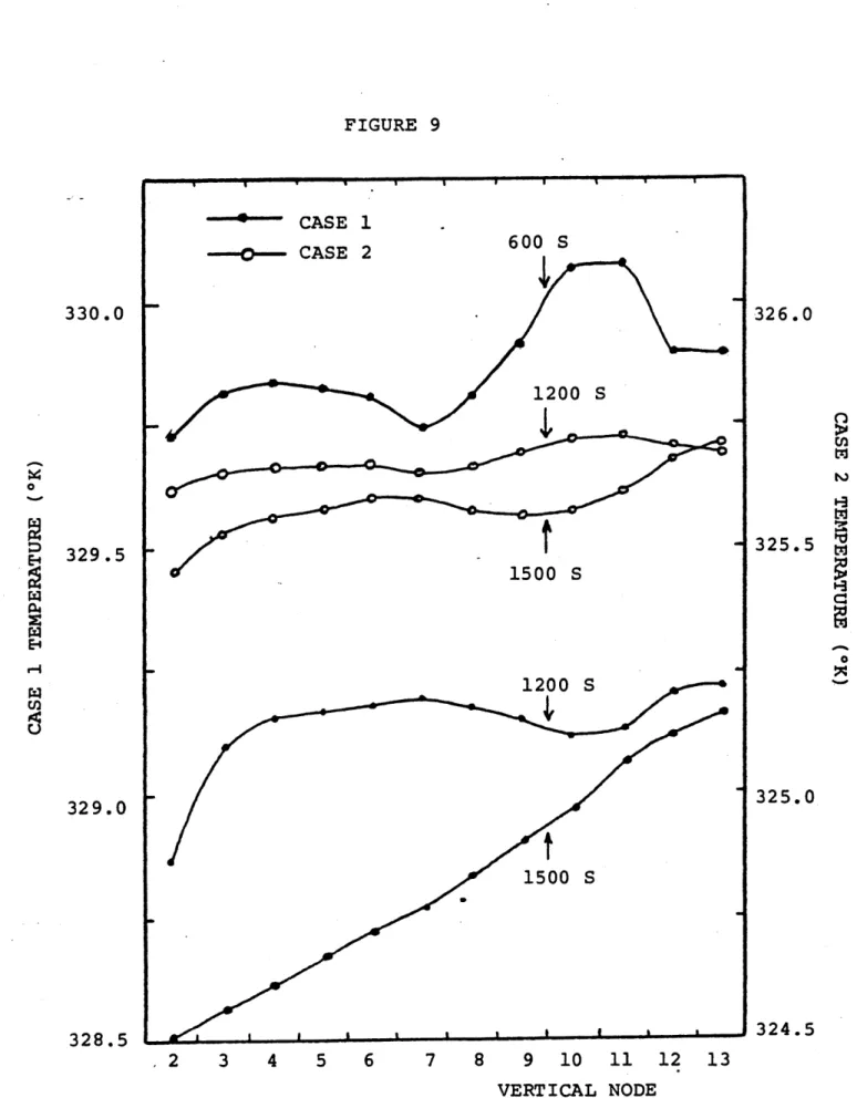
1k flow influences 1. The vertical shown in Fig. 8. s the lower d illustrates Between 1200 and 1500 anges by 8% while the e thermal gradients cases are plotted in Fig.

sed energy stable gr les of the 1500 seconds (Case 1). The air dens indicating the displacement by the 1 hydrogen. The steam profile follows the thermal gradient depicted in the the hydrogen is relatively uniformly preferential collection in the dome.

9. removal to heat sin adient. Figure 10 p

three gaseous compo ity decreases with e ess dense steam and

the saturation line previous figure. F distributed except

However, the absol

The Case ks as resents nents at levation, gi ven ina for ute 1 ly, some

hydrogen volume fraction does not vary more than a few tenths of a percent over the entire field.

This problem leads to the observation that the presence of steam in conjunction with the location of heat slabs can cause some atmospheric stratification. The stratification produced is not very strong in this case and its effect on hydrogen transport equiv

is minimal in that a nearly uniform hydrogen field is obtained in both cases. The results of these analyses lead to the expecta-tion that the stratificaexpecta-tion which is becoming evident at the end of the simulation would become more stable as time elapsed.

Problem 2 - Hydrogen Injection into High Pressure and Temperature Air Atmosphere

This problem was intended to involve hydrogen injection into an atmosphere composed of air and steam but due to a programming error, an initial pure air atmosphere at elevated pressure and temperature was assumed. Despite the fact that it was an unintended computation, the results produced from this set of initial conditio questions at end. as Problem 3. The Problem 2 was 2.737 respectively. Heat Hydrogen is injecte 1800 seconds of the The maximum v duration of 20,000 plot shows a decay decay is relatively flow field obtained

ns are The int initial x 105 sinks inter ended pres N/m2 esti air sure (39.

ng and germane to the

-steam case is reported 1 and temperature of the a 7 psia) and 385.75'K (235 were at 323.15*K ater ir in 'F), as in Problem 1. d at a rate of 0.005 kg/s dur simulation.

ertical velocity history over seconds (5.55 hours) is shown to a natural convection scale

unaffected is qualita by the tively hydr simi 1 ogen ar to s

ing the first

the simulation in Fig. 11. The velocity. The ource flow. The those of Problem 1, but the depressed rates are due to rapid early condensation

rise and diminishes the causing an inversion which blocks the

upward momentum of the incoming hydrogen. The average density vertical profile at 2000 and 20000 seconds are both plotted in Fig. 12. The two profiles are similar in that the stable strati-fication of the dome (no heat sinks) region is clearly defined and becomes stronger as time elapses. The stratification is dis-tinct from the Problem 1 experience in that this is nearly

stepwise rather than linear with increasing elevation.

The thermal gradients at various times, which are depicted in Fig. 13, are analogous to the density profiles of Fig. 12. The energy removal in the lower area is apparent. The observed temperature decay rates are 0.0011 *C/sec and 0.0003 *C/sec in the lower and upper regions, respectively. Finally, Fig. 14

shows t'he air and hydrogen densities at the end of the simulation as a function of vertical position. The expected inversion

profiles are observed.

Problem 3 - Hydrogen Injection into Steam-Air Mixture

This simulation involved a hydrogen inflow identical to that assumed in Problem 2 into an atmosphere composed of air and

steam. These conditions are specified in Table 2. The steam density and thermodynamic state at the beginning of the

calcula-tion was based on the assumpcalcula-tion of a large LOCA mass and energy source added to the containment atmosphere of Problem 1. The heat sinks were not in thermal equilibrium due to the assumed rapid change in state caused by the LOCA.

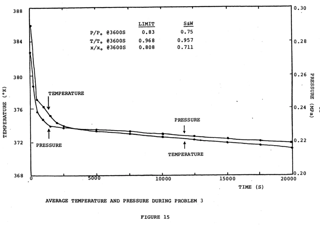
The average pressure and temperature histories over the course of the 20000 second simulation are shown in Fig. 15. The

two thermod seconds and

ynamic variables decay rapidly over the first 1500 then decrease more slowly. As a point of comparison and validation,

the steam quali down analysis u ditions were di and "final" (at agreement is ob surization in t the heat sinks. Fig. 16. This the integrated rate of over a ences (60'K) an

this pressure and temperature ty transient were compared to sing a single node model [10]. fferent for the two analyses,

3600 seconds) values are comp served. The rapid atmospheric he early period is due to rapi

This is demonstrated by the figure shows the energy remova

energy absorption of the heat megawatt is due to the initial d high heat transfer coefficie

decay as well as a large LOCA

blow-Since initial con-ratios of initial ared. Reasonable

cooling and depres-d energy removal by plots contained in 1 rate as well as sinks. The initial

temperature differ-nts (HTCs). The HTCs of the vertical heat sinks were approximately 500-600 W/m2 *K in the earlier period and decayed to r

the duration of the transient. These can values during Problem 1 of 50-70 W/m2 *K. due to elevated steam partial pressures i

The maximum velocity is plotted vs distinct regions are apparent. There is around 1000 seconds followed by a recover hydrogen source is terminated and finally steady state low flowrate. The first tra

interesting as it is not observed in the explanation of the physical phenomena cau

oughly 100 W/ be compared The higher n this case. time in Fig. an initial de y which lasts a transition nsition is th previous prob sing this beh

the flow patterns at 1000 seconds, 1750 seconds m to va ' l K for peak ues are 17. T cay un until to a e more 1 ems. av i or hree ti 1 the An is possible after

and 20000 seconds ar through 20. At 1000 different regions.

e studied. These are shown in Fig seconds, the flow pattern exhibit First, a counterclockwise recircul reminiscent of the earlier simulations,

m. Second, an area of complex flow in t exists and, finally, relatively low circ dome. This midregion pattern indicates negative buoyancy of the heat sinks and the hydrogen inflow. The flow field at much better defined counterclockwise rec nearly the entire

source-induced re recovery observed seconds shows the in Problem 1. In seems to cause a dome remains rela

The vertica similar to the Pr cation in the dom

non-dome region. The circulation is the caus

in Fig. 17. The final dual heat sink natural addition, the asymmetr smal 1 er

tively 1 densi oblem 2 e regio

flow loop in the 1 stagnant.

ty profiles depicte results with a ste n. The stratificat

s. 18 s three

at ion, exists in the lower 15 he 15 to 45 m elevation ulatory flow in the the competition of the the positive buoyancy o 1750 seconds exhibits a

irculation spanning new dominance of the e of the velocity

field seen at 20000 convection pattern fou ic horizontal heat sink

ower elevations. d in pwise ion i Fig. 21 stable s decayi are str ng f nd The atifi-(at a diminishing rate) as opposed to the stre

shorter term Problem 1 simulation. The curves of Fig. 22 reflect this stabiliza distinction from the first simulation is period, the dome region is cooling at a lower region, indicating some mixing at This is analogous to Test 6 of the BF si

ngthening observed in the temperature profile

tion. An interesting that after the initial higher rate than the the inversion interface. nce where an inversion

degraded slowly over time due to slow penetration of hydrogen gas through a small orifice.

The density profiles of all components at 1750 and 20000 seconds are presented in Figs. 23 and 24, respectively. The scales of the two figures are the same except for a small incre-mental difference in liquid density. A noteworthy feature of the 1750 second profiles is the hydrogen stratification in the lower 40 m. The profiles at 20000 seconds are similar to the former time except for more uniformity in the nondome areas, decreased dome/nondome gradients and a complete decay of the steam

gradient. The cause of the steam homogenization is probably

diffusive transport enhanced by steam removal in the lower region due to condensation. The removal of steam is evidenced in the

average steam density decreasing from 0.612 kg/m 3 to 0.560 kg/m 3 during this period.

Since flammability limits are best expressed in volume fraction rather than mass fraction, Figs. 25 through 29 are provided. Figures 25 and 26 depict the changing volumetric mixtures as time progresses for a lower elevati-on and upper

elevation, respectively. The decay in hydrogen volume fraction in the case of the former at around 2000 seconds is due to the source termination and subsequent homogenization of the lower elevations. The rapid steam condensation is also apparent. The dome region transient is notably slower and does not exhibit

rapid condensation. In fact, the steam fraction decay behaves in a way indicative of some mixing and diffusive depletion. Figures

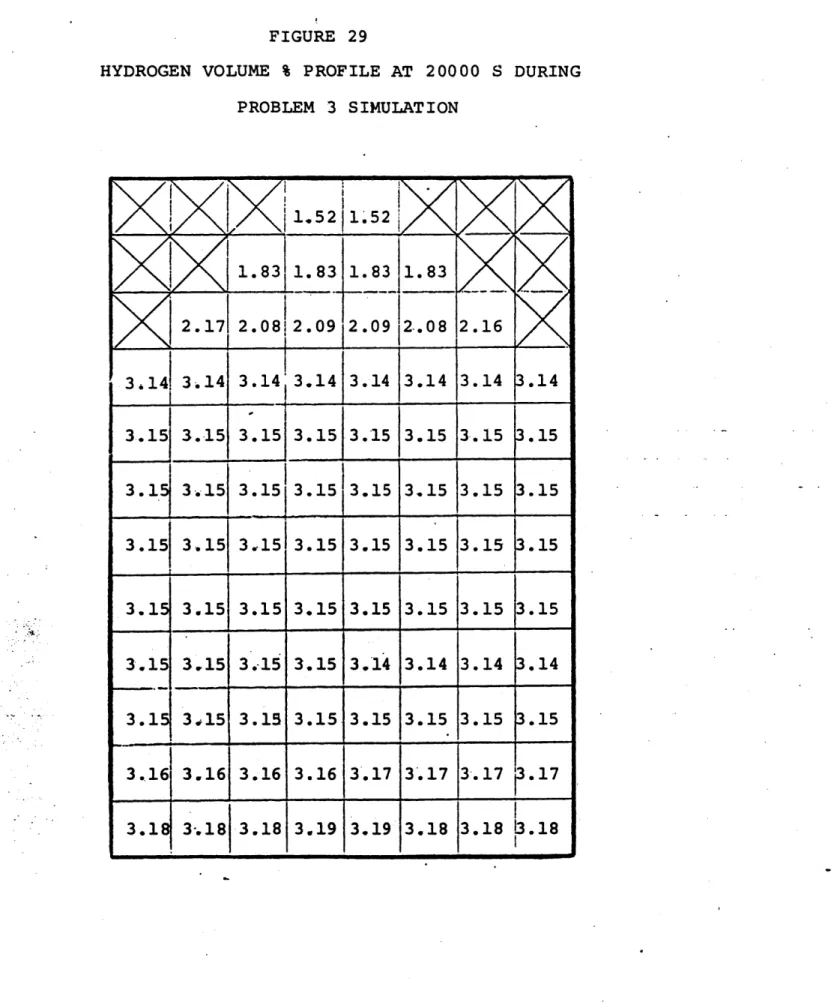
27 through 29 illustrate the whole filed "wet" hydrogen fractions (wet implies fractions computed to include steam contribution) at 1000, 1750 and 20000 seconds, respectively. The persistence of differences in the lower region during injection as well as the slow ingress of hydrogen to the dome region are noteworthy.

DISCUSSION

The results reported in the previous section demonstrate the importance of the sensitivities noted in the introductory remarks. Thermal and mass stratification is observed in certain simulations but their magnitude and exact spatial definition are sequence dependent. In the first simulation, representing a slowly degrading core sequence, a small but distinct vertically linear stable stratification formed after all sources were

removed. The presence of steam and the sequence of source

injection encouraged the formation of the stable gradients. This influence is obtained from two separate effects. First, the

initial steam injection helped heat the atmosphere and decreased the relative buoyancy of the hydrogen gas. Second, condensation heat transfer at the vertical surfaces increased the energy

removal from the bulk flow in the lower region. These heat sinks were the dynamic determinants of the post source flow transient.

Despite these modest inhomogeneities, the effect on hydrogen gas transport is minimal in this case.

The second simulation involving only air and hydrogen

showed that the heat sink energy removal could dominate the flow transient during source injection. Also, the thermal inertia

of the atmosphere is much lower when the condensible component is not present. Co

ature decreased even though the were at least an tion illustrates conditions set i

Problem 3 characteristics mixed lower volu However, this ca calculated heat this computation strongest moment nsi der 55'C, heat t order a sce n Test result i ncl ud me and se als transf due t um inf

that the nondome region average temper-while in Problem 3 the decrease was 14C ransfer coefficients in the third problem

of magnitude higher. This second simula-nario which could lead to the initial

No.6 of the BF Phase 1 series (see [14]). s share many of the second simulation's ing stepwise stable stratification,

well-dominance of heat sink energy removal. o possesses a few unique results. The

er coefficients we o the large steam

luences - negative removal and positive buoyancy

during the source injection p magnitude transient and the s The eventual smoothing of the demonstrates the importance o ent removal mechanism (i.e. c decoupling of the upper and 1

due to hyd hase as demr low evoluti vertical s f diffusive ondensation ower region re much higher mass fractions. buoyancy due t rogen inflow -onstrated by th on of the flow team density pr transport when ) is available. s with respect during The two o energy competed e velocity fields. ofile also a compon-The to hydrogen accumul at ion is also reminiscent of the BF6 test

The relevance of these results considerations is illustrated in Fig. trajectories of the three simulations combustion limit diagram. The curves limits can be violated from a variety

to hydrogen flammability 30 which depicts the

on the triagonal hydrogen indicate that flammability of initial conditions,

different subregions can differ in their flammability potential and pre-chemical reaction thermo-fluid dynamic transient deter-mines the severity of postulated burns. The impact of detailed

containment behavior on fission product transport is not addressed quantitatively in this work but the results should still be noted. A particularly important aspect is the steam density profiles observed and their potential effect on fission product removal mechanisms such as diffusiophoresis.

A number of sensitivities have not been studied although they are clearly important. First, the presence of sprays and

fan coolers would alter the outcomes dramatically. Second,

various geometries must be analyzed in order to characterize this influence. Higher priority variations include three-dimensional arrangements, different heat sink configurations and computa-tional mesh changes. A number of different accident sequences and their resultant contaminant injection transients should be simulated with the goal of distinguishing which accidents are susceptible to nonuniform containment conditions and thus require more detailed treatment than they currently receive in safety

studies.

V. CONCLUSIONS

The results of this modest investigation lead to two major conclusions. First, analysis of a few prototypic post-accident containment transients using better estimate analysis tools

indicates that atmosphere stratification and depressed mixing can be obtained. This observation is relevant to assessing safety

regulatory requirements for the mitigation of severe core damage accidents in that these results affect both fission product

transport and combustible gas control. Second, the physical con-straints that encourage or discourage atmospheric homogenization include heat sink placement, source flow, initial state and

geometrical arrangement. Much remains to be done before clear understanding of this problem is obtained. The purpose of this contribution is to stimulate attention to this important nuclear safety question.

VI. REFERENCES 1. M. A. Kenton and R. E. Henry,

Analysis Code",. Proceedings of Light Water Reactor Severe Acc MA, August 28 to September 1,

"The the ident 1983, MAAP-PWR Internat Eval uat pg. 7.3 Severe Accident ional Meeting on ion", Cambridge, . 2. R. 0. Wooton and H. I. Response Characteristic 7anual", WUREG/CR-1711,

Avci, "MARCH 1.1 (Meltdown Accident s) Code DescriptioW and UseF's

October 1980. 3. D. W. Hargroves et al., CONTEMPT-LT/028

Program for Predicting Containment Pres Response to a Loss-of-Coolant Accident, August 1978. 4. V. P. Manno and M. Containments: A Su Experiments", to be November 1984. 5. V. P. Manno et al., Hydrogen Transport Nuclear Science and

- A Computer sure-Temperature

NUREG/CR-0252,

W. Golay, "Hydrogen Transport in

rvey of Analytical Tools and Benchmark published in Nuclear Safety 25(6),

"Analytical Models for Simulating in Reactor Containment Atmospheres",

Engineering, August 1984. 6. C. R. Broadus et Thermal Hydrauli - Users Manual, al., BEACON/Mod 3: c Analysis of Nuclea NUREG/CR-1148, April 7. K. Y. Huh and M. W. Gol

Numerical Diffusion in MIT-EL-83-011, November 8. H. Uchida et al., "Eval

Systems of LWRs", Proce on Peaceful Uses of Ato

ay, Treatment Fluid Dynamic 1983. uation of Pos edings of Int mic Energy 13

A Computer Program for r Reactor Containments 1980. of Physical and Simulations, t-Accident Cooling ernational Conference (93), IAEA, 1965. 9. T. Tagami, "Interim Report on Safety

Facilities Establishment Project for Japanese Atomic Energy Agency, unpubl '10.

Assessments June 1965", ished work, Stone & Webster Engineering Corporation, private communication.

and No .1 1965.

-22-Table 1

Initial Conditions for Problem 1

Atmospheric pressure - 1.0135 x 105 N/m2 (14.7 psia) Atmospheric temperature - 323.15'K (122'F)

Composition - 100% air

Initial Velocity Field - stagnant

Table 2

Initial Conditions for Problem 3

Atmospheric pressure - 2.737 x 10 5 N/m2 _{(39.7 psia)}

Atmospheric temperature - 385.75'K (235'F) Composition - 56% air, 44% steam by mass

44% air, 56% steam by volume Initial velocity field - stagnant

40 M (1 M THICK) VERTICAL NODES 13 12 11 10 9 8 7 6 5 4 3 J = 2 HORIZONTAL NODES 60 M I= 2 3 4 5 6 7 8 9 PROBLEM GEOMETRY FIGURE 1 A

500 1000 0.03 m txI 0.02 t 0.01 ul . 0.00 1500 TIME (S) PROBLEM 1 SOURCE SPECIFICATION

FIGURE 2 F 0.8 E.4 0 44 0.6 0.4 0.2 0

3.0 V max (M/S) CASE 1 (W/ STEAM) 2.0, 1.0 0 500 1000 1500

PNOBLEM 1 MAXIMUM VERTICAL VELOCITY TRANSIENT

PROBLEM 1 SIMULATION

M ft

e_______________ e______________ k it___________

><

I

I

I

-v1ZV*A4\

\

4,

FIGURE 5

FLOW FIELD AT 1500 S DURING PROBLEM 1 SIMULATION

DENSITY STRATIFICATION OF PROBLEM 1 - CASE 1 .004 - 1500 S .002 +-1200 S en 0 E-4 H 1200 S'"*

r4

z

FIGURE 7

DENSITY SRATIFICATION FOR PROBLEM 1 - CASE 2

-.003 _{VERTICAL NODE} .003 .002 .001 0 -. 001 z 0 rz4 -. 002

0 1 1 1 - 1 1 1 1 - -1 - -1500 S

I

DURING PROBLEM 1 FIGURE 8 .010 .008 .006 .004 >4

z

FIGURE 9 326.0 txj 325.5 325.0 324.5 .2 3 4 5 6 7 8 9 10 11 12 13 VERTICAL NODE

THERMAL STRATIFICATION DURING PROBLEM 1

330.0 329.5 0 -4 CIO 329.0 328.5

FIGURE 10

2 3. 4 5 6 7 8 9 10 11

VERTICAL NODE

VERTICAL DENSITY PROFILES OF CASEOUS

COMPONENTS AT 1500 S OF PROBLEM 1 12 13 >4 H

z

z

z

z

1

0.6 Vmax (M/S) 0.4 0.2 0 5000 10000 15000 20000 TIME (S) MAXIMUM VERTICAL VELOCITY TRANSIENT

FOR PROBLEM 2

0.1 0.0 _{2 3 4 5 6 7 8 9 10 11} H

z

DENSITY SPATIFICATION DURING PROBLEM 2

380 370 360 2000 S 350 340 20000 S 330 320 2 3 4 5 6 7 8 9 10 11 12 VERTICAL NODE THERMAL STRATIFICATION DURING PROBLEM 2

.006 .005 HYDROGEN DENSITY (KG/M 3) .004 .003 .002 .001 2 3 4 5 6 7 8 9 10 11 12 13 VERTICAL NODE 2.6 2.5 2.4 AIR DENSITY (KG/M3) -4 .3 2.2 2.1

TIME (S) AVERAGE TEMPERATURE AND PRESSURE DURING PROBLEM 3

FIGURE 15 384 380 376 0 E-372 368 0.28 0.26 - n En 0.24 00 0.22 0.20

>-I 0 z 102 0 5000 10000 15000 TIME (S)

HEAT SINK ENERGY REMOVAL RATE AND INTEGRATED ENERGY ABSORPTION

DURING PROBLEM 3 2x109 ti 1x109 0 20000 106 105 10 4 103

V max (M/S) 1.0 0.5 0 5000 10000 15000 20000 TIME (S)

FIGURE 18

FLOW FIELD AT 1000 S DURING PROBLEM 3. SIMULATION

Vmax = 0.52 M/S

FIGURE 19

FLOW FIELD AT 1750 S DURING PROBLEM 3 SIMULATION

U = 0. 45 M/S

FIGURE 20

FLOW FIELD AT 20000 S DURING PROBLEM 3 SIMULATION

V M/S = 0.23 M/S

.10 .05 * 20000 S 2 3 4 5 6 7 8 9 11 12 E4

z

DENSITY STRATIFICATION DURING PROBLEM 3

1750 S

4'

20000 S

2 3 4 5 6 7 8 9 10 11 12 13

VERTICAL NODE THERMAL STRATIFICATION DURING PROBLEM 3

FIGURE 22 384 382 380 378 376

r

PROBLEM 3 SIMULATION (ALL IN KG/M ) STEAM HYDROGEN 2 3 4 5 6 7 8 9 10 11 12 13 VERTICAL NODE .80 .75 .70 AIR 1.15 LIQUID .30 1.10 .010 .008 .006 .004 .002 .000 .65 .25 1.05 .20 .60 1.00 .55 .15 0.95 .10 0.90 .05

STEAM HYDROGEN AIR LIQUID .80 .010 1.15 .35 .75 .008 1.10 .30 LIQUID 11 3 AIR .70 .006 1.05 .25 .65 .004 e 1.00 .20 HYDROGEN .60 .002 0.95 .15 STEAM .55 .000 _0.90 .10 2 3 4 5 6 7 8 9 10 11 12 13 VERTICAL NODE

55 AIR 4

rz

VOLUME FRACTION TRANSIENT FOR LOWER RIGHT HAND NODE DURING

PROBLEM 3 SIMULATION FIGURE 25

55 4 STEAM A50IR o 0o 45 2 HYDROGEN 40 35 .0 - 0 5000 10000 15000 20000 - TIME (S) VOLUME FRACTION TRANSIENT FOR DOME REGION CELL DURING

PROBLEM 3 SIMULATION

FIGURE 27

HYDROGEN VOLUME % PROFILE AT 1000 S DURING

PROBLEM 3 (WET % INCLUDING STEAM)

0.09 10.11 0.25 0.2 6 0.30 0.33

0.3810.44

FIGURE 28

HYDROGEN VOLUME % PROFILE AT 1750 S DURING

PROBLEM 3 SIMULATION 0.21 0.21 10.43 0.45 0.46 0.47

0.5710.63

I

.1 .59

FIGURE 29 HYDROGEN VOLUME PROB % PROFILE AT 20000 S DURING LEM 3 SIMULATION 1.52 1.052 1.83 1.83 1.83 1.83 2.17 2.082. 09. 2.6 _ _ _ _ 1 2 09

12

-PROBLEM 2 TRAJECTORY 100 % AIR .100% REACTION -(375K) 0 100% REACTION (410K) 10% REACTION (375K) PROBLEM 3 TRAJECTORY / DOME :TS LII4T 80 20 100% H2 80 60 40 20 100% STEAM

TRAJECTORIES OF THREE SIMULATIONS PROJECTED ON HYDROGEN-AIR-STEAM FLAMMABLILITY

MAP FIGURE 30

These computer by runs is hel Probl Probl Probl The e

Appendix - Computer Application Information

simulations ere run on the Duke Power CDC Cyber 176 Richard Jenny of uke;, The hard copy output of these d by the authors. The job names and run dates are: em 1 0-300 s (Case 1) ACGAACOH 4/26/84 300-600 s (Case 1) ACGAABFS 5/3/84 600-1500 s (Case 1) ACGAAAIG 6/20/84 0-600 s (Case 2) ACGAAAIU 6/20/84 em 2 0-20000 s ACGAAAMB 7/6/84 em 3 0-20000 s ACGAAATB 7/16/84

xecution time and efficiency statistics are summarized below Simulated _{Time (s)_} 300 300 900 600 20000 20000 42100 CPU Time (s) 476 316 764 744 3958 5061 11319 CPU time duration-cel1* 0.01888 0.01254 0.01011 0.01476 0.00236 0.00302 0.00320 *84 fluid cells Job COH BFS AIG AIU AMB ATB TOTAL