SYSTEMATIC EVALUATION AND CHARACTERIZATION OF 3D SOLID STATE LIDAR
SENSORS FOR AUTONOMOUS GROUND VEHICLES
A.K. Aijazi∗, L. Malaterre, L. Trassoudaine, P. Checchin
Institut Pascal, UMR 6602, Universit´e Clermont Auvergne, CNRS, SIGMA Clermont, F-63000 Clermont-Ferrand, France (ahmad-kamal.aijazi, laurent.malaterre, laurent.trassoudaine, paul.checchin)@uca.fr
KEY WORDS: Solid state LiDAR; Characterization; 3D point clouds; Object detection; Segmentation and classification
ABSTRACT:
3D LiDAR sensors play an important part in several autonomous navigation and perception systems with the technology evolving rapidly over time. This work presents the preliminary evaluation results of a 3D solid state LiDAR sensor. Different aspects of this new type of sensor are studied and their data are characterized for their effective utilization for object detection for the application of Autonomous Ground Vehicles (AGV). The paper provides a set of evaluations to analyze the characterizations and performances of such LiDAR sensors. After characterization of the sensor, the performance is also evaluated in real environment with the sensors mounted on top of a vehicle and used to detect and classify different objects using a state-of-the-art Super-Voxel based method. The 3D point cloud obtained from the sensor is classified into three main object classes “Building”, “Ground” and “Obstacles”. The results evaluated on real data, clearly demonstrate the applicability and suitability of the sensor for such type of applications.
1. INTRODUCTION
Lately, 3D LiDAR (Light Detection And Ranging) sensors have proved to be an integral part different autonomous nav-igation and perception applications, ever since the first imple-mentations of SLAM (Simultaneous Localization And Map-ping) for robotics (Thrun, 2002) and practical demonstrations on vehicles (Thrun et al., 2006), LiDARs have had an important role in realizing high accuracy occupancy maps and 3D point clouds. However, the introduction of new solid state LiDAR technology is gaining great interest in the scientific community. Even though these sensors have not yet fully commercialized, they still promise higher operational life, low power, small sizes and lower manufacturing costs.
In this paper, we present the preliminary evaluation results of working with one such sensor (as to date the sensor has not yet been launched). Different aspects of this new type of sensors are studied and their data are characterized for their effective utilization for object detection for the application of autonom-ous ground vehicles (AGV). The paper provides a set of eval-uations to analyze the characterizations and performances of such LiDAR sensors. After characterization of the sensor, the performance is also evaluated in real environment with the sensors mounted on top of a vehicle and used to detect and clas-sify different objects using a state-of-the-art Super-Voxel based method.
The paper aims to provide a first-hand analysis of this new LiDAR technology which is fundamental in understanding the capabilities of these sensors for different autonomous vehicle applications. In the state-of-the-art, we find that many works have evaluated different 2D and 3D LiDAR sensors like Ye and Borenstein (Ye, Borenstein, 2002) studied the character-ization of the Sick LMS 200 laser scanner while a newer ver-sion of smaller Sick lasers such as LMS-100 family were eval-uated in (Rudan et al., 2010). Similarly, the Hokuyo series was also well studied with the characterization of the
URG-∗ Corresponding author
04LX (Okubo et al., 2009) and, more recent versions, like the UTM-30LX (Hrabar, 2012).
In (Stone et al., 2004), the authors review in detail the dif-ferent types of LiDAR technologies, highlighting the differ-ent problems associated with several “off-the-shelf” LiDAR systems. The general trends in LiDAR sensor technology as well as their likely impact on manufacturing and autonomous vehicle application are also discussed. Other LiDAR tech-nologies based on rotating beam mechanism, like the Velo-dyne family, is also extensively studied. (Atanacio-Jim´enez et al., 2011) calibrated the HDL-64E using large cuboid targets while (Muhammad, Lacroix, 2010) by extracted wall surfaces. An automatic RANSAC-based plane detection algorithm was used in (Chen, Chien, 2012) for the same purpose. A more re-cent version, VLP-16, was evaluated by Wang et al. (Wang et al., 2018) and compared to cheaper RS-LiDAR manufactured by Robosense. After studying different aspects such as drift, orientation, surface color, material, etc., performance of the two sensors was reported to be similar.
Time-of-flight cameras, such as SwissRanger from Mesa Ima-ging, were characterized in (Kahlmann et al., 2006) and (May et al., 2009) and corresponding calibration models were also developed. Similarly, the authors of (Khoshelham, Elberink, 2012) characterized the Kinect sensor, used in several robot-ics applications. Not much work on 3D solid state LiDARs can be found in the state-of-the-art as it is a rather new and evolving technology. Some very recent works (Schleuning, Droz, 2020) (Ruskowski et al., 2020) just provide an over-view of the underlying technology especially in the context of autonomous driving applications. However, to the best of our knowledge no prior work on the systematic evaluation and char-acterization of such solid state LiDARs has been presented. In Section 2, we give a brief introduction of the sensor and its underlying technology and, in Section 3, we present the char-acterization results of the sensor. In Section 4, we present the experimental results in a real application while we conclude in Section 5.
Parameter Value
Technology Solid state
Range 100 m @ 10% reflectivity Field of View 65° × 30° Resolution 0.25° × 0.15° Accuracy ±2 cm Power Consumption 10 W Size 10 cm × 10 cm × 7 cm
Environmental Safety IP-68 Laser Safety Class-1 eye safe
Table 1. Specifications of the sensor F-01 2. 3D SOLID STATE LIDAR
LiDARs measure by emitting a laser beam that is reflected back from different objects and focused into a receptor to determine the corresponding distances. Traditional LiDARs are electro-mechanical devices relying on moving parts, to scan the sur-rounding environment, that need to be precise and accurate in order to obtain suitable measurements over a large field of view. The moving parts involved in the system not only result in size restrictions and increased manufacturing costs but it also im-plies that the sensor would be more susceptible to perturbations and vibrations resulting in lower operational life. However, des-pite the high cost, restrictions, and difficulty to manufacture, LiDAR is still widely used for different perception tasks. Solid state LiDAR sensors are based on silicon chip techno-logy without requiring mechanically moving parts. Apart from lower manufacturing costs, they promise higher operational life, low power and small sizes. The solid state 3D LiDAR sensors mainly employ either Micro-Electro-Mechanical Sys-tem (MEMS) technology to drive the mirror in order to redirect a single laser in different directions or a Flash array that illu-minates the entire field with a single flash.
In this work, the 3D solid state sensor used is based on a flash array type mechanism employing 905 nm wavelength laser and a time-of-flight distance measurement method. As the sensor has not yet been released in the market, it is named F-01 for convenience. The main specifications of the sensor are sum-marized in Table 1.
3. CHARACTERIZATION OF 3D SOLID STATE SENSORS
In order to characterize the sensor data, different tests were con-ducted for the study of drift analysis, effects of surface color and material, incident angle, luminosity, target distance and the phe-nomena of pixel mixing. These are described in the following parts of this section.
3.1 Drift Analysis
The drift analysis sheds light on the stability of the LiDAR. To analyze the drift effect and the stability of the 3D Solid state sensor, measurements of a plane surface was performed over a long period of time. The LiDAR was placed at a fixed distance from a white wall and kept the y-axis of the sensor vertical to the plane of the wall. The drift effect is mainly due but the rise in temperature as the device keeps working. Repeated measure-ments were taken over a period of 2 hours.
Figure 1 shows the variation in distance measurements with re-spect to the time. From the figures it could be seen that a large
variation of about 2 cm is observed in the first 20 min of run-ning.
Figure 1. Drift analysis showing the variation of distance measurement with respect to time
3.2 Effect of Surface Colors
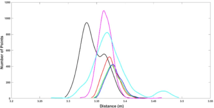
The laser is usually affected by the color of the target surface. In order to evaluate the LiDAR’s performances with respect to different colors, the three primary colors red, green, blue and two secondary colors black and white and also a shiny silver (high reflectivity) color were tested. Each of these 6 colored targets are all the same material of papers and were all fixed on exactly the same place during each test. The results, in the form of distance distributions, are presented in Figure 2.
Figure 2. Variation of distance measurement with respect to different colors. The color of the plots corresponds to the surface color except cyan represent white color and magenta shiny silver
color 3.3 Effect of Surface Material
Just like varying colors, the material of the target’s surface also has an effect on the reflection of the laser. In order to evalu-ate this effect, tests were conducted on three different mevalu-aterial target sheets. The three targets were all the same white color however the materials were different: concrete, metal and tis-sue cloth. The results are shown in Figure 3.
The variation in distance measurements observed due to differ-ent materials was not much. However, it could be seen that for the metallic surface the number of returns (reflected 3D points) were much higher.
3.4 Variation of Incident Angle
The effect of different incident angles on the range measure-ment accuracy was also studied. In all other experimeasure-ments/tests this angle was kept constant at 0°. The target (a 0.5 m × 0.5 m reflecting screen) was mounted on a precise rotary table and the central axis of the sensor and the rotation axis of the target were
Figure 3. Variation of distance measurement with respect to different materials
carefully aligned ensuring that the distance between the two re-mains constant. The target was rotated in both clockwise and anti-clockwise directions from −45° to +45°. We were not able to get reliable range measurements for angle superior to ±45° due to lack of reflected 3D points. The results are presented in Figure 4.
Figure 4. Variation of distance measurement with respect to different incident angles
It can be seen that the results are almost symmetric for the +ve and −ve angles and that the distance measurement is more ac-curate within ±30° incidence angle.
3.5 Influence of Luminosity (Ambient Light)
In order to evaluate the sensor’s performance at different lu-minosity levels, distance measurements of a fixed white target were taken. The luminosity levels were modified using a large external lamp. The corresponding luminosity levels were meas-ured using a LUX meter. The results presented in Figure 5 show that the sensor is quite robust to changes in luminosity as there is not much variation in distance measurements.
Figure 5. Variation of distance measurement with respect to different luminosity levels
3.6 Problem of Pixel Mixing
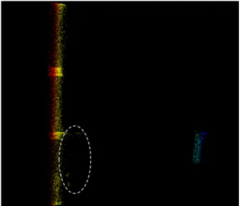
When a laser spot is located at the very edge of an object, the measured range is that of a combination of the foreground ob-ject and the background obob-ject, i.e., the range falls in between the distances to the foreground and background objects. This condition is called “mixed pixels” (Cooper et al., 2018). In order to evaluate this phenomenon, we placed a white target at about 3.1 m with a uniform background at about 5.0 m in front of the scanner as shown in Figure 6.
Figure 6. Side view of the 3D points belonging to the target (shades of blue) and uniform background. Circled in white, we
find few false points due to the problem of mixed pixels The number of false measurements (points) due to pixel mix-ing was found to be very few as shows in Figure 6 (encircled in white). These can be easily removed or filtered out in post processing.
3.7 Distance Analysis
In order to analyze the effect of target distance, we took the measurements of the same target surface at different distances (1 m to 20 m). The measured distances with respect to the ground truth are presented in Figure 7. The small measure-ment error with a standard deviation of 2.08 cm demonstrates the high precision of the sensor.
Figure 7. Measurement accuracy with respect to distance (range) 4. EXPERIMENTATION IN REAL APPLICATIONS Once the sensor data was characterized, it was also tested in real application environment. The sensor was mounted on a forklift
as shown in Figure 8. The tests were conducted in a large fact-ory shed with different types of objects placed/scattered on the factory floor. These included common objects such as cartons of different size, pallets, metallic poles, other forklifts, storage racks and pedestrian etc. The sensor mounted vehicle affected several known trajectory around these objects. The 3D point clouds obtained from the sensor were then processed to detect and classify these objects in each frame. In order to avoid the problem of ego motion the vehicle moved at slow speeds of 2 m/s, 1 m/s and 2.5 m/s.
Figure 8. The sensor mounted on top of a forklift In order to process the 3D point clouds, a state-of-the-art Super-Voxel based method (Aijazi et al., 2016) was employed. In this method the 3D points are first grouped together to form tetrahedral voxels of different sizes based on an R − NN and then properties are assigned to each of these voxels based on the constituting points. Using these properties the voxels are linked together along the three dimensions to form objects. The ground, assumed to be a large plane is extracted and then the remaining objects are classified using geometrical features. Al-though, the original work classified 5 different classes including cars and trees which are of less relevance in our application, we modified it to classify the point cloud into three main classes, i.e., “Ground”, “Building” and “Obstacles”. The main geomet-rical features used include size of bounding box, direction of surface normal and planarity, etc. All objects that could be an obstacle for the moving vehicle are included into the class called “Obstacles”. Some results are presented in Figure 9 and Table 2 shows the evaluation results using standard metrics like Accuracy (ACC) and F1 measure (F1) using (1) and (2)
re-spectively.
ACC = TP + TN
TP + TN + FP + FN (1)
where TP, TN, FP and FN are True Positives, True Negatives, False Positives and False Negatives, respectively.
F1 = 2 × Precision × Recall Precision + Recall (2) where Precision = TP TP+FP and Recall = TP TP+FN. In order
to evaluate these metrics, analysis was done using 3D points of the different object classes. The high accuracy results clearly demonstrate the applicability and suitability of the sensor for such type of applications.
5. CONCLUSION
In this paper we present the preliminary evaluation results of a solid state LiDAR sensor. Different aspects of this new type
ACC F1
Building 0.941 0.929 Ground 0.901 0.892 Obstacles 0.895 0.868 Table 2. Evaluation of classification results
of sensor are studied and their data are characterized for their effective utilization for object detection for the application of autonomous ground vehicles (AGV). The paper provides a set of evaluations to analyze the characterizations and perform-ances of such LiDAR sensors. After characterization of the sensor, the performance is also evaluated in real environment with the sensors mounted on top of a vehicle and used to de-tect and classify different objects using a state-of-the-art Super-Voxel based method. The highly accurate results (with ACC about 90%) clearly demonstrate the applicability and suitability of the sensor for such type of applications.
ACKNOWLEDGEMENTS
This work was sponsored by a public grant overseen by the French National Agency as part of the “Investissements d’Avenir” through the IMobS3 Laboratory of Excellence (ANR-10-LABX-0016), the IDEX-ISITE initiative CAP 20-25 (ANR-16-IDEX-0001) and by the Auvergne-Rhˆone-Alpes re-gion.
REFERENCES
Aijazi, A. K., Serna, A., Marcotegui, B., Checchin, P., Tras-soudaine, L., 2016. Segmentation and Classification of 3D Urban Point Clouds: Comparison and Combination of Two Approaches. D. S. Wettergreen, T. D. Barfoot (eds), Field and Service Robot-ics: Results of the 10th International Conference, Springer Tracts in Advanced Robotics, Springer International Publishing, Cham, 201–216.
Atanacio-Jim´enez, G., Gonz´alez-Barbosa, J.-J., Hurtado-Ramos, J. B., Ornelas-Rodr´ıguez, F. J., Jim´enez-Hern´andez, H., Garc´ıa-Ramirez, T., Gonz´alez-Barbosa, R., 2011. LIDAR Velo-dyne HDL-64E Calibration Using Pattern Planes. Interna-tional Journal of Advanced Robotic Systems, 8(5), 59. ht-tps://doi.org/10.5772/50900. Publisher: SAGE Publications. Chen, C.-Y., Chien, H.-J., 2012. On-Site Sensor Recal-ibration of a Spinning Multi-Beam LiDAR System Using Automatically-Detected Planar Targets. Sensors, 12(10), 13736– 13752. https://www.mdpi.com/1424-8220/12/10/13736. Num-ber: 10 Publisher: Multidisciplinary Digital Publishing Institute. Cooper, M. A., Raquet, J. F., Patton, R., 2018. Range Informa-tion CharacterizaInforma-tion of the Hokuyo UST-20LX LIDAR Sensor. Photonics, 5(2), 12. https://www.mdpi.com/2304-6732/5/2/12. Number: 2 Publisher: Multidisciplinary Digital Publishing In-stitute.
Hrabar, S., 2012. An evaluation of stereo and laser-based range sensing for rotorcraft unmanned aerial vehicle obstacle avoidance. Journal of Field Robotics, 29(2), 215–239. ht-tps://onlinelibrary.wiley.com/doi/abs/10.1002/rob.21404. Kahlmann, T., Remondino, F., Ingensand, H., 2006. Calibration for increased accuracy of the range imaging camera SwissRanger. Proceedings of the ISPRS Commission V Symposium ’Image En-gineering and Vision Metrology’, XXXVI Part 5, ISPRS, 136– 141. Accepted: 2019-10-10T07:15:05Z ISSN: 1682-1750. Khoshelham, K., Elberink, S. O., 2012. Accuracy and Resolution of Kinect Depth Data for Indoor Mapping Applications. Sensors,
(a)
(b) (c)
Figure 9. (a), (b) and (c) show the classification results. In blue are the 3D points classified as “Ground”, in green are the 3D points classified as “Building” and in red are the 3D points classified as “Obstacles”
12(2), 1437–1454. https://www.mdpi.com/1424-8220/12/2/1437. Number: 2 Publisher: Molecular Diversity Preservation Interna-tional.
May, S., Droeschel, D., Holz, D., Fuchs, S., Malis, E., N¨uchter, A., Hertzberg, J., 2009. Three-dimensional mapping with time-of-flight cameras. Journal of Field Robotics, 26(11-12), 934–965. https://onlinelibrary.wiley.com/doi/abs/10.1002/rob.20321. Muhammad, N., Lacroix, S., 2010. Calibration of a rotating multi-beam lidar. 2010 IEEE/RSJ International Conference on Intelligent Robots and Systems, 5648–5653. ISSN: 2153-0866. Okubo, Y., Ye, C., Borenstein, J., 2009. Characterization of the Hokuyo URG-04LX laser rangefinder for mobile robot obstacle negotiation. Unmanned Systems Technology XI, 7332, Interna-tional Society for Optics and Photonics, 733212.
Rudan, J., Tuza, Z., Szederk´enyi, G., 2010. Using LMS-100 laser rangefinder for indoor metric map building. 2010 IEEE Inter-national Symposium on Industrial Electronics, 525–530. ISSN: 2163-5145.
Ruskowski, J., Thattil, C., Drewes, J. H., Brockherde, W., 2020. 64x48 pixel backside illuminated SPAD detector array for LiDAR applications. M. Razeghi, J. S. Lewis, G. A. Khoda-parast, P. Khalili (eds), Quantum Sensing and Nano Electronics and Photonics XVII, 11288, International Society for Optics and Photonics, SPIE, 36 – 46.
Schleuning, D., Droz, P.-Y., 2020. Lidar sensors for autonomous driving. M. S. Zediker (ed.), High-Power Diode Laser Techno-logy XVIII, 11262, International Society for Optics and Photon-ics, SPIE, 89 – 94.
Stone, W. C., Juberts, M., Dagalakis, N., Stone, J., Gorman, J., 2004. Performance analysis of next-generation LADAR for man-ufacturing, construction, and mobility. Technical Report NIST IR 7117, National Institute of Standards and Technology, Gaithers-burg, MD.
Thrun, S., 2002. Robotic Mapping: A Survey. G. Lakemeyer, B. Nebel (eds), Exploring Artificial Intelligence in the New Mil-lenium, Morgan Kaufmann.
Thrun, S., Montemerlo, M., Dahlkamp, H., Stavens, D., Aron, A., Diebel, J., Fong, P., Gale, J., Halpenny, M., Hoffmann, G.,
Lau, K., Oakley, C., Palatucci, M., Pratt, V., Stang, P., Stro-hband, S., Dupont, C., Jendrossek, L.-E., Koelen, C., Markey, C., Rummel, C., Niekerk, J. v., Jensen, E., Alessandrini, P., Bradski, G., Davies, B., Ettinger, S., Kaehler, A., Nefian, A., Mahoney, P., 2006. Stanley: The robot that won the DARPA Grand Challenge. Journal of Field Robotics, 23(9), 661–692. ht-tps://onlinelibrary.wiley.com/doi/abs/10.1002/rob.20147. Wang, Z., Liu, Y., Liao, Q., Ye, H., Liu, M., Wang, L., 2018. Characterization of a RS-LiDAR for 3D Perception. 2018 IEEE 8th Annual International Conference on CYBER Technology in Automation, Control, and Intelligent Systems (CYBER), 564–569. ISSN: 2379-7711.
Ye, C., Borenstein, J., 2002. Characterization of a 2D laser scanner for mobile robot obstacle negotiation. Proceedings 2002 IEEE International Conference on Robotics and Automation (Cat. No.02CH37292), 3, 2512–2518 vol.3.