Allocation algorithms for real-time systems as applied to battle management

Allocation Algorithms for Real-Time Systems as

Applied to Battle Management

by

Kin-Joe Sham

Submitted to the Department of Electrical Engineering and Computer

Science

in partial fulfillment of the requirements for the degree of

Master of Engineering in Computer Science and Electrical Engineering

at the

MASSACHUSETTS INSTITUTE OF TECHNOLOGY

May 2002

©

Kin-Joe Sham, MMII. All rights reserved.

The author hereby grants to MIT permission to reproduce and

distribute publicly paper and electronic copies of this thesis document

in whole or in

part.

OF TECHNOLOGY

JUL

31

20j

LIBRARIES

A uthor

..

_{. .. ... ....}

_.

.. ..

...

..

_..

....

. ..

.

Department of Elec~ical Engineering and Computer Science

%\ May 24, 2002

Certified by

...

...

...

Dr. Leslie P. Kaelbling

Professor of Computer Science and Engineering, MIT

Thesis Supervisor

Certified by...

...

Dr. Michael E. Cleary

The Charles Stark Draper Laboratory, Inc.

Teclii6alj$upervisor

Accepted by ..

...

Dr. Arthur C. Smith

Chairman, Department Committee on Graduate Students

Allocation Algorithms for Real-Time Systems as Applied to

Battle Management

by

Kin-Joe Sham

Submitted to the Department of Electrical Engineering and Computer Science on May 24, 2002, in partial fulfillment of the

requirements for the degree of

Master of Engineering in Computer Science and Electrical Engineering

Abstract

The ability to distribute the proper number of weapons and planes depending on the available information and resources is crucial in a successful air strike campaign. Current algorithms for this problem domain such as Yost's hybrid approach and the Markov task decomposition (MTD) approach model the given problem using Markov decision processes, but only in minimal detail for computational feasibility. This thesis extends the MTD approach to more closely match realistic situations. The new technique introduces different weapon types and incorporates constraints on the number of planes available and the number of weapons each plane can carry. Although it is impossible to prove that solutions produced by the modified MTD approach are close to optimal for large-scale problems, tests have shown that the modified MTD approach generates solutions with higher expected utility compared to other heuristics. Experiments were also conducted to determine the effect of varying each element in an allocation problem on the algorithm's overall computation time. The results demonstrated that only the off-line phase significantly increases its running time due to the extension. Thus, real-time distribution analysis is possible since the on-line phase requires a negligible amount of time to execute.

Thesis Supervisor: Dr. Leslie P. Kaelbling

Title: Professor of Computer Science and Engineering, MIT Technical Supervisor: Dr. Michael E. Cleary

Title: Principal Member of the Technical Staff, The Charles Stark Draper Laboratory, Inc.

Acknowledgements

I would like to thank my Draper Laboratory supervisor, Dr. Michael E. Cleary, for

all his help and technical advices, which assisted me in completing my thesis. In addition, I am grateful to him for accepting me into the Draper Fellowship program and providing me an interesting topic to research on.

I would also like to thank my thesis advisor, Professor Leslie P. Kaelbling, for

the constant feedback and technical support that she offered. Without her expertise in the stochastic planning problem domain, my research would not have went as smoothly as it did.

Acknowledgements [continued]

This thesis was prepared at The Charles Stark Draper Laboratory, Inc., under the Internal Research and Development Program (Account #18556).

Publication of this thesis does not constitute approval by Draper Laboratory of the findings or conclusions contained herein.

stimulation of ideas.

(Author's signature)

It is published for the exchange and

Assignment

Draper Laboratory Report Number T-1428.

In consideration for the research opportunity and permission to prepare my thesis

by and at The Charles Stark Draper Laboratory, Inc., I hereby assign my copyright of

the thesis to The Charles Stark Draper Laboratory., Inc., Cambridge., Massachusetts,

--- --

512±J~

Contents

1 Introduction

15

1.1 Battle Management Scenario... . . . .. 16

1.2 General Statement of The Problem . . . . 16

1.3 Approaches . . . . . . . . . . 17

1.3.1 Linear Programming Approach . . . . 17

1.3.2 Partially Observable Markov Decision Process and Linear Pro-gramming Hybrid Approach . . . . 18

1.3.3 Markov Task Decomposition Approach with On-Line and Off-Line P hases . . . . . . . . . . . . 20

1.4 Experim ental Design . . . .. 21

1.5 Thesis Contributions . .. . . . . 22

1.6 Thesis Organization . . . .. 22

2 Technical Background

25

2.1 Markov Decision Process (MDP) . . . . 25

2.1.1 The M DP M odel . . . . 26

2.1.2 Value Iteration Solution Method . . . . 27

2.2 Markov Task Decomposition (MTD) . . . . 29

2.2.1 Off-line Value Table Calculations . . . . 30

2.2.2 Online Value Maximization . . . . 31

3 Markov Task Decomposition with Only a Global Constraint

33

3.1 M odel Formulation... . . . . . . . . 33

3.2 Modification to MTD Approach . . . . 3.3 Architecture Overview . . . .

3.4 Implementation Details . . . . 3.4.1 Damage State Model . . . . 3.4.2 Battle Management World . . . 3.4.3 Off-Line Value Function Tables 3.4.4 On-Line Policy Mapper . . . . .

3.5 Replication of Meuleau's Results . . . .

4 Mar

4.1 4.2 4.3

kovian Task Decomposition with Multiple

New Additions to the Modified MTD Approach Architecture Improvements . . . . Implementation Details . . . . 4.3.1 Weapon Types . . . .

4.3.2 Available Planes and Weapons per Plane

Constraints

Constraints

5 Experimental Results

5.1 Experimental Approach . . . . 5.2 Modified MTD Algorithm vs Other Heuristic

5.3 Effect of Model Changes . . . .

5.3.1 Additional Targets . . . .

5.3.2 Additional Target Types . . . .

5.3.3 Multiple Damage States . . . . 5.3.4 Additional Weapons . . . .

5.3.5 Additional Weapon Types . . . .

5.3.6 Additional Planes . . . .

6 Conclusions and Future Research Areas

6.1 Conclusions . . . . 6.2 Potential Applications . . . . 6.3 Future W ork . . . . 34 34 36 36 37 39 39 40

43

43 44 45 45 48

51

51 53 54 54 57 58 59

60

61

63

63 64 64 . . . . . . . . . . . .

List of Figures

1-1 Yost's Decomposition Algorithm [9] . . . .

19

3-1 Markov Task Decomposition Approach . . . . 35 3-2 An instance of optimal policy for single-target problem using Meuleau's

approach [8](left bars), or using the MTD approach (right bars) . . . 41

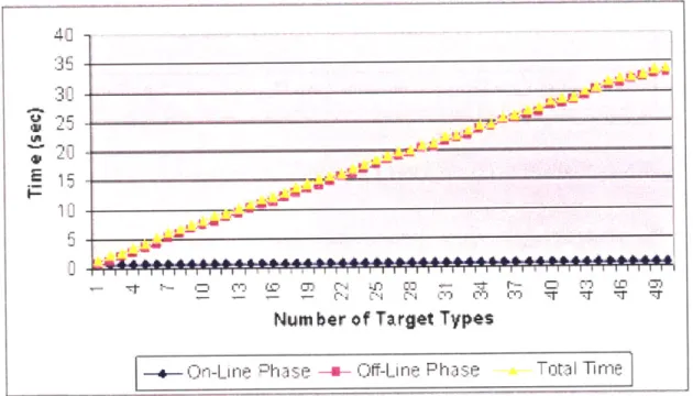
5-1 Comparison of the quality of policies generated by Modified MTD and Greedy Strategy for a 100-target problem . . . . 53 5-2 Modified MTD's running time with a varying number of targets. . . . 56 5-3 Modified MTD's running tirne with a varying number of target types. 57

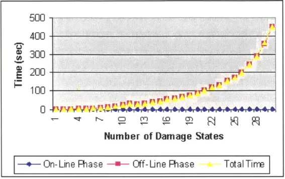
5-4 Modified MTD's running time with a varying number of damage states. 58

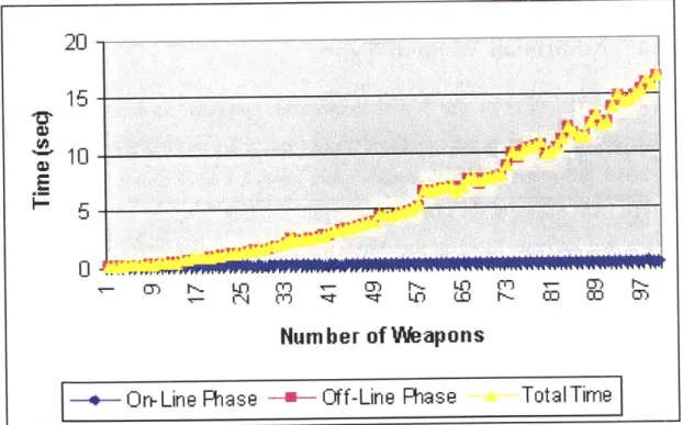
5-5 Modified MTD's running time with a varying number of weapons. . . 59 5-6 Modified MTD's running time with a varying number of weapon types. 61

List of Tables

5.1 A list of variables and their corresponding values for each experiment. 52 5.2 A summary of the resulting trends seen in the computation time by

Chapter 1

Introduction

Finding efficient ways to distribute limited resources is an problem that can be found in many different domains. Although techniques such as linear programming have already been used to tackle general deterministic allocation problems, they have not been successfully applied to allocation problems where allotting resources to objects can change the state of the object based on its stochastic model. This type of problem is illustrated in a range of areas, from distributing doctors within a hospital to running a successful business corporation. One of the places where this is a major problem, however, is in the military.

The ability to take appropriate actions depending on the available information and resources is crucial to the success of military campaigns. Typically, combat mission design will attempt to make good use of resources such as the limited number of fighting units and weapons. However, with so many different variables involved in a real battle, it is difficult to allocate the appropriate amount of resources and determine the best sequence of actions to maximize the enemy's damage while incurring the lowest associated costs. The work described herein is undertaken with the goal of making the process of allocating resources more effective by using miore sophisticated mathematical models of battle environments. Following a statement of the problem in section 1.2, several allocation methods are described in detail in section 1.3.

1.1

Battle Management Scenario

The particular resource allocation problem in a combat scenario that is being exam-ined can be described as follows. There are limited numbers of available weapons and strike aircraft with associated costs, which need to be assigned to attack a set of enemy targets within a finite time horizon that varies per target. Each target has two observable states, dead or alive. Furthermore, there is an a priori reward for a target being in each of the two states. At any given time interval t, a certain number of weapons and strike aircraft can be allocated to a target. The target's state in the next time interval t + 1 is determined by a probability function based only on the target's current state and the allocation given in time t. In this model, each target is independent of the other targets, thus changing the state of a target will not affect the outcome of other allocations.

1.2

General Statement of The Problem

The domain of the allocation problem described above has several important traits. First, there are fixed amounts of various resources (e.g., weapons and aircraft) and a finite set of objects (e.g., targets), where each object has a known number of states.

A limited set of actions, each of which consumes probabilistic amounts of available

resources, causes objects to change states. There is an a priori reward for having an object in each of its possible states. The total value of the solution at a given time step can be calculated by summing the expected rewards for each object. Time is divided into discrete intervals over a finite horizon and actions can be applied to each object in each time interval. Since every action uses resources, the actions performed on each object must be constrained so that in total they consume less than the total available resources at every time interval and over the entire time horizon. A global constraint is defined as a restriction that is enforced over the entire time horizon (e.g., the limited amount of resources). An instantaneous constraint is another type of constraint that can also be incorporated into the problem. The constraint must be

independently satisfied at each time interval (e.g.., the limited number of planes and the holding capacity of each plane). This problem domain is modelled with an Markov decision process (MDP) where actions change the states of objects probabilistically[7].

It is assumed that the objects are all independent of each other, implying that the Markov models are all independent. However, the overall problem cannot be solved without merging together the solution to each independent MDP because the objects are still competing for the same pool of resources. For further discussion of Markov models, see section 2.1.

1.3

Approaches

A feasible solution to the resource allocation problem can be obtained using known

heuristics [9] that determine reasonable weapon distributions. However, such meth-ods do not give information on the effectiveness of the allocation. Using a feasible solution derived from a heuristic could be sufficient in certain applications, but if a better solution is used. additional resources could be saved for future missions. Cur-rently., there are several different methods being researched to solve the problem in the battle management scenario. This section will describe three of the techniques being explored and demonstrate how each technique focuses only on part of the entire prob-lem. The three are the linear programming (LP) approach, the off-line POMDP and LP hybrid approach created by Yost, and the Markov task decomposition approach established by Meuleau. ct al.

1.3.1

Linear Programming Approach

Currently, the military applies methods such as linear programming (LP) [5] to al-locate resources in weapon/plane allotment problems similar to the problem within the battle management scenario. Linear programming is a commonly used approach because it maximizes or minimizes linear functions with many variables to obtain the desired optimal results within a finite set of constraints. However, these deterministic techniques do not capture the probabilistic elements in the problem, since a

determin-istic resource allocation does not take into account the damage state of the enemy targets and the probability that the weapons applied to the targets could miss or fail to damage them sufficiently. To incorporate these probabilistic elements and the sequential decision making into the model causes the problem to become immediately intractable for even simple problems [9].

For example, let's assume that each target can only be dead and alive and a global state of the model is a combination of each target's status, then the total number of global states |SI is |S| = 21TI where ITI is the number of targets. Thus, with each

target added to the model, the problem grows exponentially because the number of states ISI increases by a factor of two for each new target. This is assuming that total probabilities must be computed for all the possible combinations of alternatives to find the optimal solution to any probabilistic problem. Hence, even a reasonably small problem with a probabilistic model can take significant computation to solve using only linear programming [9].

1.3.2

Partially Observable Markov Decision Process and

Lin-ear Programming Hybrid Approach

Research has been done on ways to find the optimal solution for problems that re-quire allocating resources among activities that either gather information on different objects or take actions in an attempt to change the state of these objects [6]. The model described here can be directly applied to the battle management scenario by viewing the problem as a weapon and sensor allocation problem where sensors can observe targets and weapons can cause damage to the targets. As mentioned in the previous section, using linear programming to find the optimal answer will make even a small-scale problem intractable since every probabilistic combination must be examined.

To further complicate the problem, it may be impossible to get complete infor-mation about the state of the objects. Another way to say this is that the state of the objects is only partially observable

[7].

Such a problem can be modelled with one

large partially observable Markov decision process (POMDP) [2]. However, a POMDP is significantly more complicated than a MDP and becomes intractable much more quickly than the linear programming approach. In order to overcome this challenge, small independent POMDPs can be used to model the behavior of individual targets. Yost constructed a decomposition procedure shown in Figure 1-1 that combines linear programming (LP) and POMDPs to determine the resource allocation strategy, in addition to finding the optimal policy for each target [9]. A policy in this case is a sequence of sensor action and weapon usage.

Ini tial _{Current object values,}

Policies _{resource marginal costs}

MASTER LP POMDP

available resources

object constraints optimal policy for

current costs

Improving policies _improvi Quit when no_{ng policies} are found.

Figure 1-1: Yost's Decomposition Algorithm [9]

The approach uses linear programming to compute the marginal costs of resources, which is the cost for using one additional resource. Then each POMDP takes these costs to determine an optimal policy for allocating resources to the targets of its type. The resulting policies are sent back to the master LP which allocates these policies to targets and recalculates the marginal costs. The iterative loop is terminated once the overall optimal policy is discovered [9].

Although an exact solution can be found, the entire calculation process is ex-tremely time-consuming for a large-scale problem, so it is computed off-line.

There-fore, this method cannot be used for real-time analysis or decisions.

1.3.3

Markov Task Decomposition Approach with On-Line

and Off-Line Phases

To decrease the computation time for solving large-scale problems, Meuleau, et al.,

[8] created the Markov Task Decomposition approach to separate the solution process

into two phases, allowing the more time-consuming calculations to occur separately from the actual algorithm for allocating weapons. The result is a relatively fast technique that can find near-optimal solutions to distribute weapons for maximizing the targets' damage. Due to the stochastic nature of the objects' states, Markov decision processes (MDPs) are used to model individual targets in this approach. However, unlike the hybrid approach, the technique assumes that all information about the targets is completely observable, thus MDPs are used instead of POMDPs.

A MDP is created to model a system and is defined by a set of states and a set of

probabilistic rules that governs the object's state transitions. The model is applied to problems that describe a series of dependent trials such as a sequence of events and decisions made based on the current status at each time step [3]. The MDP model and solution process is explained in more detail in section 2.1.

If a large-scale problem is modelled with one MDP, then it would be intractable due

to the amount of computation needed in the traditional dynamic programming tech-nique [1] to solve the problem. Like the hybrid approach in section 1.3.2, Meuleau's method is to decompose the large MDP into a set of smaller MIDPs. However. in-stead of solving the set of smaller MDPs and constructing a global solution using LP all in a single computation process, Meuleau first calculates a set of value function tables off-line that correspond to each sub-MDP. These offline values represent the expected utility or reward for every action taken in every state that the target could be in at each time interval under various assumptions about how many weapons will be allocated to the target in the future. Using the value function tables, an on-line allocation algorithm will optimize the distribution of weapons among all the targets

in order to maximize the expected reward [8].

One advantage of this method is that it is able to analyze real-time situations, since the deterministic allocation algorithm that distributes weapons can be solved in a relatively short amount of time. This is because a significant portion of the calculation is from the value function formulation of the stochastic processes, which are done off-line. The real-time analysis uses the value tables created off-line to combine the results of all the sub-MDPs in a deterministic manner. Furthermore, once the value function tables have been created for the different weapon/target combinations, they can be reused if a similar situation occurs again.

Despite its tractability, Meuleau's model of the battle management scenario is very simple. It did not take into account more realistic constraints such as the fact that there is a limited number of available planes and that each plane can carry only a certain number of weapons. It also did not model more than one type of weapon. Therefore, future work can extend this promising weapon allocation technique to model a more practical scenario which is what this thesis is focusing on.

1.4

Experimental Design

To examine the tractability of the modified approach discussed in this thesis, exper-iments are conducted to test the effect of changing different aspects of the model. The following variables are increased incrementally in order to observe the change in computation time: " Targets " Target Types * Damage States " Weapons " Weapon Types * Planes

The solution time for the off-line phase will be compared to the time spent on the on-line phase in order to determine which phase needs to be improved upon in future work.

1.5

Thesis Contributions

The main goal of this thesis is to extend Meuleau's approach to more closely match real-life situations. The thesis makes the following contributions in the process of achieving the main objective:

* Introduction of different weapon types, which makes the model more realistic.

" New constraints, such as a limit on the number of bombs per plane and a cap

on the number of planes available, are incorporated.

" Development of a new greedy algorithm that incorporates the above constraints.

1.6

Thesis Organization

The remainder of this thesis is organized as follows:

Chapter 2 provides the technical background information including a detailed description of a Markov decision process (MDP) and an explanation of Meuleau's allocation algorithm.

Chapter 3 presents the infrastructure of the simulator and describes the imple-mentation of the entire system.

Chapter 4 examines the online and off-line components of the system including the various new constraints that were implemented to make the model mnore realistic. The allocation algorithm used to solve the different constraints are also explained in detail.

Chapter 5 describes the different scenarios used for testing the effect of varying different components of the model and the results of the simulations.

Chapter 6 presents conclusions drawn from this research., discusses potential

ap-plications of the techniques developed in previous chapters, and presents ideas for future work that could extend the work reported here.

Chapter 2

Technical Background

Since this thesis describes several extensions that were made to Meuleau's approach

[8]. it is important to have a clear understanding of his original allocation algorithm. Section 2.1 describes the Markov decision process (MDP), which is the model used for the weapon/plane allocation problem. In addition, the section also explains the value iteration method used to solve such a process. Section 2.2 discusses Meuleau's method, which divives the off-line value iteration method used for computing the value tables using dynamic programming and the on-line value maximization technique for allocating resources. Both phases are important, since the extensions in this thesis require modifications of the value table formulation and the value maximization algorithm.

2.1

Markov Decision Process (MDP)

Choices are made based on information that has uncertainty associated with it. As-suming that events exhibit some degree of regularity, their uncertainty can be de-scribed by a probability model. The Markov decision process (MDP) is a way of characterizing a series of dependent probabilistic trials that has an unique property in the way future events are dependent on past events, where the state of each ob-ject in the next time interval is only dependent on its current state and the current action [3]. A solution to a MDP is called a policy, which indicates the action that

needs to be performed depending on the current status of the MDP and past events that occurred [7]. The MDP model will be described in more detail in section 2.1.1. Although MDP can model a stochastic problem, a method is needed to solve it. The value iteration method is a common technique used for solving MDPs and will be explained in section 2.1.2.

2.1.1

The MDP Model

Consider an object that may be described at any time as being in one of a set of N

mutually exclusive states. For the state of an object to change, an action must be performed within a finite set of actions that is allowed to take place at the given state. When an action does take place, the object may undergo a state transition according to a set of probabilistic rules given by the transition matrix. In this formulation, he transition matrix is static, which means that the probabilistic rules are independent of time. A distinctive feature of any Markov process is that the transition probabilities for a series of dependent state transitions satisfy the Markov condition. This condition states that the conditional probability of the object being in state s at time t is only dependent on the state of the object at time step t,_1 [3]. In another words. the present state of the object encompasses all the historical information relevant to the future behavior of a MDP. Thus, the transition probability for state s to change to state s' due to an action a can be represented by Pr(s'la, s).

Formally, an MDP is defined by a 4-tuple, < S, A, T, R > where S is the set of discrete object states {si, 82 ... , sn} and A is the set of available actions

{at,

a2. ..., am}. Note that the set of available actions is the collection of existing

actions at the current state. A collection of probabilistic rules also known as the transition matrix is denoted as:

T = { Pr(s'la, s) : acA, scS, s'cS}, (2.1) which specifies the likelihood that the state of the object will change from s to s' due to action a. Finally, the set

R

=

{rs,.f : 8, s'ES}

(2.2)

represents the reward space of the process. In particular, r ,,, is the reward acquired when the object is in state s and transition to state s'. Note that the reward could have a negative value which would represent a positive cost.

2.1.2

Value Iteration Solution Method

An MDP, as specified in section 2.1.1, provides a mathematical model of a dynamic system, but not methods to determine the best course of actions for the system to take. A solution to such a model requires finding a policy, which is a rule for taking actions that maximizes the rewards received or minimizes the cost sustained. More formally defined, a policy for an MDP is a mapping from the current state to a set of actions for all time periods. Since the model only defines rewards for single transitions, but the aim is to maximize the expected reward attained at the end of the global finite time horizon H, a method for finding the optimal value of a state over time needs to be defined.

The optimal value of a state, V(s, 1), is the expected sum of rewards rt at time t that will be gained over the time horizon if the transitions follow the optimal policy

7r,

H

V(s, 0) := max E Y: rt .(2.3)

Since 7 is unknown, V(s, t) is determined by solving the simultaneous equations

V(s, t)

=

max K

[T(s, a, s')(V(s', t + 1) + R(s,

'))]

-

C(a)

,

VsES

(2.4)

where To is the transition probability represented in equation 2.1. R() is the transi-tion reward described in equatransi-tion 2.2 and C(a) is the cost of the actransi-tion performed. This function states that the value of state s at time t is the expected value at the

next time t + 1 minus the cost of taking the best available action when in state s, for

all possible states

[7].

For a given state s and a given time t, there exists an action that maximizes the value function. The optimal policy, therefore, is mapping of states to best available actions that satisfy the optimal value function in equation 2.4:

7r(s, t)

=

arg max

[Z[T(S,

a., s')(V(s', t + 1) + R(s, s'))]

- C(a)j

VsES,

(2.5)

where a can be any action that is available in state s at time t. The policy 7F is determined for every possible state over the entire time horizon H to formulate a table of actions that corresponds to the policy of the MDP. Equations 2.4 and 2.5 can be solved simultaneously so that when the maximum value at a given state and time is determined, the corresponding action that gave the maximum value is stored as the best available action in the policy.

To find the optimal value function for a finite time-horizon H, the simultaneous equations can be solved using dynamic programming through an iterative algorithm called value iteration. The value of being in any state at the final time is assumed to be zero,

V(s. H)

=

0. VscS,

(2.6)

because the MDP only models events up to the time-horizon and not events at the time-horizon or beyond. Thus, using equation 2.6, as the base case, the equations can be traversed backwards from H to time zero to calculate the optimal values. For example, since T(s, a,

s'),

_{R(s, s') and C(a) are all known, equation 2.4, at time H-i1,}

can be reduced to,

V(s, H

-

1)

=

max 1

[T(s, a, s')R(s,

s')] - C(a)j ,VSES

where all the values at time H - 1 are computable. This iteration will occur until

Equations 2.4 and 2.5 are observed to have a solution time that grows at an order of

O(1

A -. S12_{). This illustrates that the computation time grows linearly with} respect to the number of actions JAI and polynomially with respect to the number of states ISI, since each additional state introduces another equation in the simultaneous equations. However, when multiple objects are described by a single MDP, where a global state is a combination of each object's state, the computation time of the iteration value method will explode. This is due to the fact that the global state space grows exponentially with respect to the N number of objects such that O(IS N), as described in section 1.3.1. Because realistic descriptions of real-life problems involves many objects, the state space S can have countless number of global states, making computational tractability an issue. Therefore, new ways for solving MDPs have been explored such as the Markov Task Decomposition method.

2.2

Markov Task Decomposition (MTD)

Although MDPs are valuable in modeling stochastic planning problems such as weapon/plane allocation to targets, the computational time of the value iteration method grows

ex-ponentially when dealing with multiple objects, making large state and action spaces intractable. One technique for solving a large MDP is called the Markov Task De-composition method [8]. MTD separates a large MDP with concurrent processes into their own individual sub-MDPs and then merges the solutions to approximate a global solution. This dramatically reduces the solution time since each sub-MDP has exponentially smaller state and action spaces that can be solved in a relatively short amount of time compared to the full MDP. The tradeoff for using MTD is that the computed policy is not optimal. However, it has been shown empirically that MTD produces policies for small problems that are close to the optimal results [8].

The problem with MTD is the difficulty in combining the policies from each sub-MDP effectively. The rewards and transition probabilities of each concurrent process are assumed to be independent. This assumes that an assignment of resources to one task does not affect the expected utility of another task. However, this is sometimes

not the case since global or instantaneous constraints can tie the sub-MDPs together, making the algorithm to combine the local policies a non-trivial task. The MTD approach sacrifices optimality for faster computational time.

MTD is performed in two phases. An off-line phase (§2.2.1) solves the sub-MDPs associated with individual tasks by calculating the respective optimal value functions and the associated optimal policy using the value iteration method. An online phase (§2.2.2) uses the optimal policies determined in the off-line phase to maximize the overall value based on the current state. The resources that maximized the overall value are then assigned to each task, which would perform the best available action according to its local policy [8].

2.2.1

Off-line Value Table Calculations

The value of a state can vary, depending on the action that is performed at that state. To find the optimal value of a state, an action must be selected that would maximize the value at a given time with a given allocation by comparing values derived from each action. When an action a is taken at time t, a reward r is received for transitioning from the current state 5 to another state s'. In addition to the reward, the value V(s', t + 1. m - a) must also be considered, for being in s' at time

t + 1 with the remaining allocation after the action a is executed. The expected value

for going to the resulting state s' is the sum of the transition probability from s to s' due to action a multiplied by the reward plus the expected value of s'. Since taking an action will typically incur a cost, the final value is the expected value for the resulting state minus the cost of the action, as shown in equation 2.4.

Now consider a MDP that is separated into N individual tasks, each having its own sub-MDP. For task i where si is the current state of the task and rij is the amount of resources allocated to the task, the Bellman equation, for the optimal value function is:

Vi(si, t, mi)

=

imax [z

[T (si, a, s')(V (s', t + 1, riu

-

a) + R(si, s'))

-

c - a

(2.7)

where action a must be less than or equal to the allocation mi given to the target. This equation for a single task is derived from the more general value function, equation 2.4.

Since the process has a finite time-horizon where 0 < t < H, all the values at the

time-horizon H are assumed to be zero as explained in section 2.1.2. Using

V (sj,

H,rmn) = 0, VsjES, 0 < m <

M,

0 < i < N (2.8)

as the base case, one can use dynamic programming [5] to compute a sub-table of expected cumulative rewards for each task. The resulting ISI x H x AJ x N table, V, will consist of all the optimal values of each task for being in each state at each time when allocated 0 < m < MI resources.

Besides calculating the off-line value table, the off-line phase also creates a table of actions. Each task has its own optimal policy that is determined when computing the value function. The best action at a given state, time and allocation is the action that maximizes the value. When a maximum value for a set of variables is calculated, the corresponding action is extracted. Derived from equation 2.5, this can be formally stated as

ai

=

arg

max

[Ti(si.,

a, s)(V(s', t + 1, mi

-

a) +

J?(si.,

s))]

-

c - a ,VscS.

(2.9)

Thus, if one knows the current state of task i, and the resource mni allocated to it at time t, then it is possible to find the best available action ai associated to the optimal value,

V(si, t, mi). Notice that the off-line phase only takes into account one

resource type. In Chapter 4, multiple resource types will be considered.

2.2.2

Online Value Maximization

Using the table V constructed in the off-line phase, the online phase allocates the resources to each task accordingly., in order to maximize the total value of the process. From the declared set of allocations, and the optimal values of each task, a set of

actions A =< al, a2, ..., ai, ... > is extracted from the action table created in the off-line phase. There are many ways to perform this value maximization, however most algorithms are either sub-optimal or not computational feasible.

In this thesis, a greedy algorithm adopted from Meuleau's work is used for the online value maximization. Even though the algorithm does not promise an optimal solution, Meuleau gave empirical evidence that the solution is better than the solu-tions produced by other known heuristics

[8].

The greedy algorithm is adapted for a weapon-to-target allocation problem where a constraint on the number of weapons is present. Given the current state s _{of all targets, the number of weapons remaining M,}

and the time t, the objective is to choose mi, the number of weapons assigned to each target i with state si, so that the sum of 1K(si, mi, t) is maximized and E mi < M.

To solve the value maximization problem, the marginal utility AK of assigning an additional weapon to target

i

given that mi weapons have already been allocated to it is defined as

A V(si

mi,

t)

=

V(si

mi

+ 1, t)

-

(5i, mi,

t).

(2.10)

Weapons are assigned one by one to the target that has the highest A / for the current allocation of mi. Once a weapon is allotted to target

i,

an updated AV is computed for the next marginal utility with a new allocation of mi + 1. The method terminates when all M weapons have been distributed or AV(si, mi, t) < 0 for all

i.

This is a reasonable assumption because the marginal utility function for a given target is monotonically decreasing such that there is never a situation where adding an additional weapon will decrease the expected utility but adding six weapons will suddenly increase the utility. Because the process above is a gradient ascent on E Vi, it could be trapped in a local maximum, thus resulting in a sub-optimal allocation. Again, notice the greedy algorithm in this case is only adapted for one weapon type and no plane types or plane (instantaneous) constraints. The algorithm will be modified in Chapter 4 to handle these constraints.

Chapter 3

Markov Task Decomposition with

Only a Global Constraint

The Markov Task Decomposition approach established by Meuleau, et al, solves

weapon allocation problems with only a single global constraint. Section 3.1 de-scribes a representation of the battle management scenario that can be solved using the MTD approach. In order to apply this technique to air strike campaigns with different types of targets., changes were made to the original approach while maintain-ing the smaintain-ingle global constraint criteria. These adjustments are identified in section 3.2 and the system architecture of the modified MTD algorithm are described in 3.3. Furthermore, section 3.4 explains the various modifications made in the simulator implementation to accommodate for the changes in the MTD approach. The per-formance of the revised method is determined by comparing it to the original MTD technique's since the two approaches should arrive at the same solution when weapon allocation problem only has one target type. The result of this experiment will be discussed in section 3.5.

3.1

Model Formulation

The battle management scenario creates an environment for solving military campaign planning problems. Each target in the scenario is represented by an individual task

modelled with an independent sub-MDP. The global constraint in the problem is the total number of weapons available for the campaign. To solve the stochastic planning system, the online phase merges the policies of each sub-MDP sub-optimally without violating the global constraint. The overall policy determines the actions taken on each target, which have inherently probabilistic outcomes. The result is completely observable, meaning that the information received after an action is taken is accurate. The model formulation here is very flexible, thus additional amendments such as plane and instantaneous weapon constraints described in Chapter 4 can be made with little difficulty.

3.2

Modification to MTD Approach

Adjustments were made from Meuleau's approach to create a more realistic model of the battle management world under a global resource constraint. In the modi-fled model, there are different target types, where each type has its own transition probability matrix, reward for being destroyed, and number of damage states. These features will be discussed in more detail in section 3.4. Furthermore, multiple targets in the environment can be represented by the same target type. The battle manage-ment scenario allows targets to have windows of vulnerability within the time-horizon. The goal of the system created here is to produce a sub-optimal policy for distributing a limited number of weapons for attacking targets that appear within various time intervals within the finite time-horizon.

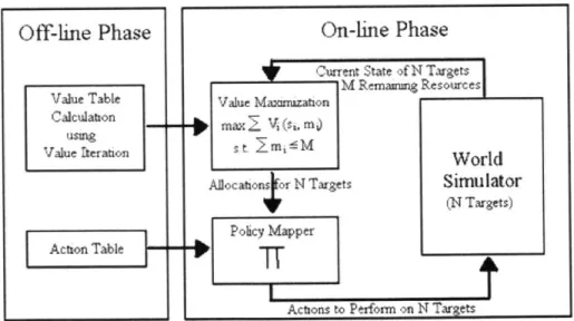
3.3

Architecture Overview

The system constructed with the changes stated in section 3.2 can be divided into three distinctive sections: the online phase, the value function tables, and the simu-lator. The value function tables for each target type are computed off-line using the value iteration method during the initialization of the system's environment. This procedure requires the transition matrix, reward for being destroyed, and the set

of damage states that describes the sub-MDP of each target type. Although

the

on-line value maximization looks up the value tables at every time step, the value

computations are only carried out once during the off-line phase. Thus, the off-line

section saves a significant amount of running time by not having to calculate a value

in real-time whenever the value is needed by the value maximization method.

After the table calculations are completed, the system begins its on-line simulation

with the world simulator. The simulator presents the current states of all the targets,

the current time step, and the remaining resources to the on-line value maximization

algorithm. The algorithm will then maximize the overall value greedily to establish

a good resource allocation. The results are passed into the policy mapper,

which

decides the action that needs to be taken on each target, in terms of the amount

of

weapon allocated to it. The actions that are taken on the active targets are passed

back to the world simulator. This allows the simulator to probabilistically determine

the resulting state of each active target after performing the assigned action. The

loop is repeated until the time step reaches the final time horizon. Figure 3-1 shows

a flow diagram that illustrates the operation of the system.

Off-line Phase

Value Table Calculatton USU19 Value rteraion Acbon Table

Figure 3-1: Markov Task Decomposition Approach

On-hne Phase

c twe=4 _{Id Remaa} State 4 1 Targets_Resources

Value Maxnuaton

2 May- V (i n)

21 MWorldIm

Allocabons Or N Targes Simulator

(N Targets) Poicy Mapper

3.4

Implementation Details

The implementation of the system described here requires several unique components. The simulator, called the battle management world, offers an environment for mod-elling existing targets. The means of interaction between the model and the real-time decisions made by the MTD approach are provided by the world simulator. For each target, a damage state model is used to determine the status of the target in a proba-bilistic manner. The most important parts of the system are the off-line value tables and the on-line policy mapper. These components are necessary for solving the large-scale stochastic planning problem. The sections below will describe each component in detail.

3.4.1

Damage State Model

The damage state model is used to describe the severity of the damage done to a target. The status of a target

i

is established as one of the states in the set of all possible damage states. This set of damage states is modelled mathematically by

Si = {u,

d

1

,

..., dN}, where u is undamaged, and d, to dN are the degree of harm

inflicted on the target with d, being the least damage done and dN being the most. If the target is damaged during its window of opportunity, the current state of the target is changed to the state representing the severity of damage, and a certain amount of reward is received, depending on the amount of damage done. When a change of state occurs, it can only go from a lesser damage state to a higher damage state.

A single weapon can damage a target

i,

causing a change in its damage status from state di to state dj, with a probability of P(di -- dj). The transition probability

matrix for one weapon is given in the initialization file. From this, a "noisy-or" model is assumed for multiple weapons, in which a single strike is sufficient to inflict damage on the target. More specifically, since individual weapons' strike probabilities are independent, when several weapons hit a target at one time step, they can all potentially cause different levels of damage to the target. It is assumed, however, that the damage status of the target is equivalent to the highest level of damage

triggered by one of the multiple weapons landed on the target. For example, if all three weapons cause the damage status to jump from d3 to d5 independently, then

the target's condition is equal to d5. However, if instead, one of the three weapons

causes the damage status to jump from d3 to d4, then the target's current state is

equal to d6.

The transition probability matrix for multiple weapons can be derived from the single weapon transition probability matrix that is given (luring the initialization of the system. Assuming PI(di -+ dj) is the probability of one weapon causing the

damage state to jump from di to dj then,

Pa(di

->

dj)

==

-

K

P (di -- d Pa(di a -+ d) (3.1)

k-imj+

This equation states that the sum of all the strike probabilities using a weapons starting from the initial state of di is equal to 1. To find the probability of Pa(di d).,

the probabilities of Pa(di -+ di) to Pa(di -> d_ 1 ) and Pa(di --4 dj tj) to Pa(di dIsI)

should be subtracted from 1. The expression, E -1 P (di -+ dk)]a, is the combination of all single weapon probabilities that causes the state to change from di to dk for 0 k

j-1,

which equals to the sum of probabilities of Pa(di -+ di) to Pa(di -> d-t). Subsequently, the expression., El,'

Pa(di

--> d,) is the sum of Pa(di -- dj I.1) to

aP

(di -

d~s).

To solve the equation above, dynamic programming is used. The base case is when

r

=

IS,

thus setting

z.<csta"

Pa(di -- dm) to 0. This leaves

Pa(di ->dIsl) = I - 1 PI(di - d )

i+

(3.2

k=0

which can be calculated from the information given at initialization. The loop will allow one to compute all the probabilities, Pal for every possible state transition.

3.4.2

Battle Management World

The battle management world is initialized at the beginning of a simulation. The world contains a set of distinct target types, a set of targets, the available resources

remaining, and the current time step. Targets with the same target type are indistin-guishable from each other since they are modelled by the same sub-MDP. However, all the targets exist at different window of availability which is the period of time when they are vulnerable to an attack. Thus, at a given time step, some targets can be attacked but others will not be available for an air strike. Each target type is initialized by computing its damage state model as shown in section 3.4.1. The target type also indicates the amount of reward received for causing a damage state change.

During the on-line simulation, the set of targets and the available resources are all updated at each time step. When the on-line phase of the MTD approach determines a set of action to be taken on the active targets, it is passed back into the simulator to update the world.

To find out the resulting state for a given target i, the vector of probabilities for transitioning from the current state di after taking an action ai is extracted V =<

Pa(di - di), ... , Pa(di -' dmaxgtate) >. Notice that the vector components add up to 1 as stated in the previous section. A random number generator picks a number between 0 and 1. If the number is between E k--I Pa(di -- dk) and Zdi/3 Pa(di - dk)

then the resulting state for the given target i is dj. For example, assume that there are 3 states and the target is currently in damage state dj, then the vector of transition

probabilities might look like, Vp =< 0. 0.2, 0.8 >. There is a zero probability to go

back to the undamaged state. a 0.2 probability for staying in the same state dj, and a 0.8 probability for the target to be completely destroyed d2. If the random number

generator picks a number between 0 and 0.2, then the resulting state is damage state dj. However, if the generator picks a number between 0.2 and 1.0, then the final state is damage state d2 (completely destroyed).

Besides updating the current state of the targets, the remaining resources also need to be computed. The new amount of resources is

wher = o - E a, _(3.3)

resources after taking the set of actions provided by the policy mapper.

3.4.3

Off-Line Value Function Tables

In this planning problem, the computation for value function tables can be noticeably simplified compared to the generic off-line value calculation discussed in section 2.2.1. Since every target of the same target type is indistinguishable from each other, only a single table is computed for each target type and not for each target. The only difference between the targets is their window of opportunity. For a target i whose window of availability is from t to t + k, then the value function for that target corresponds to the value function of its target type from H - k to H, where H is the

finite time horizon. Another simplification that can be made is that the value is 0 for every target type whose status is "destroyed". Thus, it is unnecessary to compute those values.

From the value tables, it can be shown that V(si., mi, t) increases monotonically with m until it plateaus at m*J. This is the point where the marginal utility of allocating one more weapon is zero and the marginal utility of using an additional weapon is negative. This implies that even when a weapon is allocated at this point, it will never be used because the cost of the weapon outweighs the benefit of using it. Since it is known that the values beyond m* remain constant, the off-line value calculations only need to be evaluated to that point. The values past that allocation should simply be set to the value at m*t,, instead of calculating the values using the value iteration method. This is another way to significantly decrease the computation

time of the off-line phase.

3.4.4

On-Line Policy Mapper

The policy mapper implements the value maximization algorithm specified in section 2.2.2 and searches to find a set of actions that maximizes the expected utility given a set of allocations. Using a greedy strategy, the on-line phase allocates weapons to each active target in order to maximize E V(si, mi, t). The weapon allocation is then

passed to the search command, which looks up the action ai to be taken on each target

i using V and mi as indices. Each action ai maximizes

V

given the current state,

the allocation and the time. The array of actions A =< a1, ..., an > is executed in the simulator which stochastically determines the resulting states S =< si, ... , s, >.

Note that it is never optimal to drop all the allocated weapons at once, which will be explained in the next section.

3.5

Replication of Meuleau's Results

In order to demonstrate that the MTD approach described in this chapter arrives at the same quality of policy as the original MTD approach, the same problem is given to the two models and the policies of the two approaches are compared. The problem consists of a single target that has a window of opportunity spanning over the entire time horizon where

U

= 10. In this case, the target can only be in two

states, either undamaged or danaged. Furthermore, the probability of hitting the target is pi = 0.25 and the reward received for damaging the target is ri = 90. Only one weapon type is available and the cost of using the weapon is c = 1. With the given scenario, the same number of weapons are sent at time t in both approaches assuming the target is still undamaged. Thus., the result verifies that the MTD approach described here produces the same quality of policy compared as Meuleau's approach.

In figure 3-2, the two approaches are shown to deliver an increasing number of weapons at each step as the window of opportunity comes to an end. Since the probability of damaging the target only depends on the number of weapons used at the time and not the order in which the weapons are used, the number weapons sent at each time step is increased since there is less time to damage the target in the future if the weapons sent at the next time step miss again.

Figure 3-2: An instance of optimal policy for single-target problem using Meuleau's

approach

[8](left

bars), or using the MTD approach (right bars)

12

S.

10-1

MeuIeau's

Approach

4

m

Modified WD

2

Approach

z

1

2 3 4 5 6 7 8 9

Tim

e

Chapter 4

Markovian Task Decomposition

with Multiple Constraints

In order to construct a more realistic model, several features and constraints are added to the MTD described in Chapter 3. Section 4.1 lists the modifications and explains how each one relates to a limitation seen in realistic situations. Minor changes are also made in the architecture of the simulator so that it can support the additional features. Furthermore, the algorithms used in the on-line and off-line phases of the MTD approach are extended from the previous chapter to include the new constraints. These changes are discussed in section 4.2 and section 4.3, respectively.

4.1

New Additions to the Modified MTD Approach

Several new features are introduced to more realistically model air strike campaigns. The ability to have different weapon types is included in the modified MTD approach to model the various weapons that could be used in an air strike. Each weapon type has different damage capabilities depending on the target type it hits. This concept is discussed in further detail in section 4.3.1. Another attribute added is that only a limited number of weapons can be delivered by one plane to attack a single target on a given time step. Specifically., there is a finite supply of planes, where each plane has a defined weapon capacity. Weapons are distributed among the targets by plane

loads. Once all the planes are assigned to the different targets at a given time, no extra weapon can be used for a strike at that instance even if it could increase the expected utility. The goal of the system created here is to produce a near-optimal policy for distributing a limited number of weapons carried by a specified number of planes for attacking targets that appear within the finite time-horizon the target's vulnerability window.

4.2

Architecture Improvements

The basic components of the system designed here are similar to the architecture described in Chapter 3. However, minor changes in the simulator, the on-line phase and the off-line phase are made in order to adapt the MTD model to the new scenario. Since the new model introduces multiple weapon types, the total number of weapons for weapon type j is stated as Mj. In this model, the simulator still assigns a weapon allocation to each target at every time step. The only difference is that a weapon allocation for target i is now comprised of an array of weapons Wi,

Wi =<w,'w 2, ... ,WK > , w <_ Wj

<

M1 f or 1 <

j

< K. (4.1)

where K is the number of weapon types, and W1 is the amount of remaining weapons of type

j.

The set of weapons that is dropped on a target is defined as the action A taken on a target i, which is characterized by

Ai

=< a,

a2,, aK > aj

< wj for

1

<j <

K, (4.2)

where wj is the number of weapons of type

j

allocated to target i and aj is the number of weapons being dropped. Note that a weapon allocation

Wi

is the number of weapons assigned to a target over the entire time horizon H, but an action assignment

Ai

_{is the number of weapons that is used on a target at a given time step. For example,}

if there is a total of 5 weapons of type I and 6 weapons of type II, then a possible weapon allocation for a given target i is

Wi

=< 2, 3 >. When action Ai =< 1, 2 >