HAL Id: hal-02955627
https://hal.univ-grenoble-alpes.fr/hal-02955627
Submitted on 11 May 2021HAL is a multi-disciplinary open access archive for the deposit and dissemination of sci-entific research documents, whether they are pub-lished or not. The documents may come from teaching and research institutions in France or abroad, or from public or private research centers.
L’archive ouverte pluridisciplinaire HAL, est destinée au dépôt et à la diffusion de documents scientifiques de niveau recherche, publiés ou non, émanant des établissements d’enseignement et de recherche français ou étrangers, des laboratoires publics ou privés.
Distributed under a Creative Commons Attribution - NonCommercial - NoDerivatives| 4.0 International License
Fault Detection and Isolation for Proton Exchange
Membrane Fuel Cell Using Impedance Measurements
and Multiphysics Modeling
G. Jullian, Catherine Cadet, S. Rosini, M. Gerard, V. Heiries, Christophe
Bérenguer
To cite this version:
G. Jullian, Catherine Cadet, S. Rosini, M. Gerard, V. Heiries, et al.. Fault Detection and Isolation for Proton Exchange Membrane Fuel Cell Using Impedance Measurements and Multiphysics Modeling. Fuel Cells, Wiley-VCH Verlag, 2020, 20 (5), pp.558-569. �10.1002/fuce.202000022�. �hal-02955627�
Fault detection and isolation for Proton Exchange Membrane
Fuel Cell using impedance measurements and multiphysics
modelling
G. Jullian1,2, C. Cadet2,* , S. Rosini1, M. Gérard1, V. Heiries3, C. Bérenguer2
1 Univ. Grenoble Alpes, CEA, LITEN, DEHT, F-38054 Grenoble, France
2 Univ. Grenoble Alpes, CNRS, Grenoble INP, GIPSA-lab, 38000 Grenoble, France
3 Univ. Grenoble Alpes, CEA, LETI, DSYS, F-38054 Grenoble, France
Abstract
This study proposes a model-based tool for fault detection and isolation for Proton Exchange Membrane Fuel Cell (PEMFC) for embedded applications that is robust to behaviour changes due to power demand fluctuations and stack ageing. The considered faults are the abnormal operating conditions that can shorten the fuel cell lifetime. The fault detection approach is based on residual generation using both voltage and high frequency resistance measurements and thus combining the advantages of knowledge-based model and EIS diagnosis approaches. To that end, a multi-physics fuel cell model has been used. This model computes not only the stack voltage but also the high frequency resistance in dynamic conditions. Additionally, the model is modified to take into account the ageing of the fuel cell. Validation is carried out on experimental characterizations during 1,000 hours ageing. The results on a new fuel cell stack show a score of 91% for fault isolation. However, this score drops dramatically while the stack is ageing. Finally, thanks to ageing modelling, diagnosis performances remain reliable during fuel cell stack ageing.
Keywords: PEM Fuel Cell, Fault Diagnosis, Electrochemical Impedance Spectroscopy (EIS),
1 Introduction
Fuel cell systems are very interesting devices for powering electrical vehicles with a range comparable to classical vehicle and without pollutant emission. While system’s powers are reaching the global targets for massive deployment, cost and durability remain the main issues of this technology. Degradation phenomena of fuel cell systems leading to performance losses are widely studied in literature [1,2] and their links with operating conditions have been demonstrated [3]. On one hand, poor water management dramatically increases the degradation rate and therefore shortens fuel cell lifetime [4]. Furthermore, the humidity level is either too high, occurring flooding of the channels and electrodes, or too low that causes membrane drying. On the other hand, fuel and air starvation also dramatically increases the degradation rate [5]. The fuel cell system ancillaries, composed of air compressor, valves, humidifiers, cooling system are used to control the stack operating conditions. These operating conditions (temperature, humidity and partial pressures) must be monitored and abnormal operating conditions must be identified as soon as possible and without any error. However, the fuel cell behaviour changes during ageing due to degradations. In order to maintain the fault detection performances during all the fuel cell lifetime, fault diagnosis methods need to take stack ageing into account. The faults to be detected can be defined as operating conditions that result in a decrease in the power delivered by the stack, which can cause significant damage to the fuel cell stack. Those faults can be the result of actuator faults, sensor faults, as well as system or stack components faults. Currently, various diagnostic approaches are being used [6,7] that can broadly be split into data-based and model-based methods. In model-based approaches [8-11], the model is the outcome of the comprehensive understanding of the stack and its inner phenomena which are expressed thanks to relations of different natures (electrochemical, thermodynamic, thermal, electrical and fluidic). In this approach, an on-line comparison between the real behaviour of the stack and the simulation of the dynamic model is conducted. In case of detecting a significant discrepancy (i.e. a non-zero residual) between the model and
the sensor measurements, the existence of a fault is assumed. An advantage of model-based methods is that they are robust against system modifications and the same method can be applied to different stacks. Additionally, as the model parameters have a physical meaning, simulation of ageing phenomena can be quite straightforward [12]. However, some points weaken the relevancy of this approach. Firstly, it is complicated to establish an accurate fault diagnosis model because of fuel cell complexity, and the diagnosis performance is highly dependent on the model accuracy. Secondly, knowledge-based models have high-computational demand, which can be a disadvantage for real-time embedded applications. These are the reasons why data-based methods are also developed. In data-based methods [13-19], an algorithm is trained to recognize default signatures using data collected on real fuel cell during a learning phase. The advantages of these methods are that there is no need of an accurate model of the fuel cell behaviour and that they are easy to implement. However, the performances are deeply linked to the quality and the quantity of the available collected data. In the search for fault indicators that are significantly sensitive to the faults, many measurements can be used, as pressure drop [20] or electromagnetic field [21] for example, but the majority of the approaches are based on electrochemical measurements, and more especially Electrochemical Impedance Spectroscopy (EIS) characterisation. Indeed, it is especially well adapted to evaluate many internal phenomena depending on the frequency of the stimulus signal [22,23]. These phenomena are of three kinds. In the low frequency part, the mass transport mechanisms have the most impact. For intermediate frequencies, the main phenomena are related to charge transfer. For high frequencies, the impedance can be assimilated to a resistance, mainly depending on membrane water content [24,25]. Firstly, equivalent circuit models have been developed so as to reconstruct the entire EIS characteristic [26,27], but as there are no direct relations between the proposed equivalent circuit elements and physicochemical properties of the fuel cell, interpretation reaches some limits [28]. That is why the current studies get interested in extracting features from EIS measurement [25,29,30].
However, a remaining lock is the difficulty to propose EIS measurements without disturbing the fuel cell operation, especially for low frequencies [28,31,32]. At last, a remaining obstacle is that there are no fault detecting algorithms for fuel cells that are robust to the change in impedance spectrum due to degradation [33] . A link between EIS characterisations and fuel cell ageing has been established, as in e.g. [34]. However, it is not desirable to use features that change with time, since the adaptation of the diagnosis algorithm becomes then difficult. In this work, we propose a fault detection and isolation tool for Proton Exchange Membrane Fuel Cell (PEMFC) for embedded application and robust to behaviour changes due to power demand fluctuations and stack ageing. To that aim, a multiphysics and multiscale model [12,35] is used. An advantage is that the validity of the model can be extended to the whole life, by adjusting parameters depending on the stack ageing. Besides, model-based approaches and EIS characterisations have not so far been used jointly together in diagnosis methods, though these tools are complementary. In our approach, in order to allow transposition of the tool in embedded situations with few adaptations, the measurements have been limited to only voltage and high frequency resistance that can also be simulated by the model. In fact, measuring fuel cell impedance for a large range of frequencies is difficult in real-time conditions because it takes a long time to record the signal, especially for low frequency. However, some reliable solutions have been proposed to characterize online the high frequency part of the impedance without disturbing the fuel cell operation [30,32]. Interestingly, the high frequency part of the impedance is linked with relative humidity, and it is also dependant on the electrochemically active surface area, whose variations are correlated with aging phenomena [28]. Finally, for the isolation step, a supervised classifier has been chosen as it can be used easily in real-time on an embedded system. However, the model is still used to train the algorithm offline, so that there is no need to embed the complete model itself, but only the classifier. In this way, the approach remains valid for ageing stages. Thus, the contribution of this work is the proposal of a complete fault detection and diagnosis tool, which is robust to power demand and stack ageing, and use
several diagnosis approaches [36]. The diagnosis tool is tested on five different faults that can greatly damage the fuel cell stack. These faults are related to a change in the temperature, relative humidity of the inlet gases, pressure and stoichiometry. In the following parts, the fault detection and isolation methods are described. The experiments carried out and the multiphysics model are then presented. Finally, the detection and the isolation results are displayed and discussed, first for a new fuel cell stack, and then for different ageing stages.
2 Experimental
2.1 Fault detection and isolation (FDI) method
2.1.1 Proposed approach
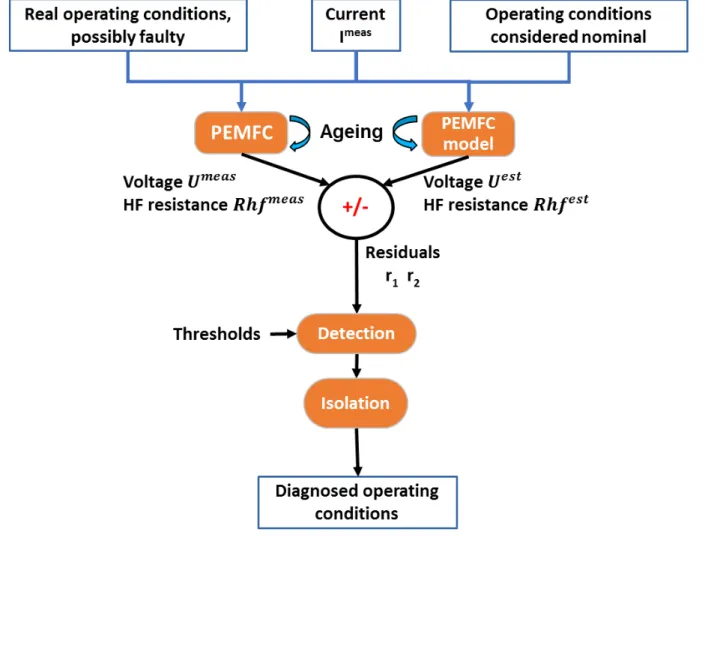
The classical model-based FDI [37] used in the present work is shown in Figure 1. This method consists of running a fixed model in parallel with the real system. Then, the outputs predicted by the model are subtracted from the same measured quantities of the real system to calculate the residuals. If the model and the real system receive the same inputs and the operating conditions are nominal, the residuals should be zero. However, it never happens because of modelling assumptions, model uncertainties and measurement noise. In addition, when a fault occurs the magnitude of one or more residuals increases. Thus, a fault is detected when the absolute value of one or more residuals is higher than a threshold value that has to be determined. The residuals which correspond to detected faults can be directly used to identify the faulty operating condition.
2.1.2 Residual generation
The originality of our proposed approach lies in the generation of the residuals. The model used in this work is the MEPHYSTO-FC [12,35], a complex multiphysics and multiscale model that has been designed to characterise fuel cells. It is a 2D+0D fuel cell model based on lumped and
bond graph approaches. It takes into account gas diffusion, two phases flow, heat transfer and electrochemistry. The complex in-plane serpentine flow field of the bipolar plates can be modelled in 2D. The through-plane species transports are modelled in 1D (no in-plane transport in the GDL and catalyst layer). MEPHYSTO-FC is used to calculate the local conditions and current distribution over the surface of the cell in response to dynamic operating conditions. Degradation mechanisms are added (by bottom-up of top-down approach) to calculate the fuel
cell lifetime under dynamic load cycles. The model can compute both the output voltage Uest,
and the high frequency resistance Rhf est. During operation, the fuel cell stack provides current to the load whereas its internal operating conditions (pressure, stoichiometry, temperature) are regulated by the stack system. Moreover during simulation, the model only takes into account the measured current provided to the load, all other operating conditions being considered as nominal. The other data that could also be collected, such as actuator or sensor values, are not used as model inputs because they can cause faulty operating conditions. The residuals r are defined as the difference between the measured values and the estimated using Eq.1 :
𝑟 = $𝑟𝑟! "% = &
𝑈#$%&− 𝑈$&' 𝑅ℎ𝑓 #$%&− 𝑅ℎ𝑓 $&',
(1)
where U is the cell voltage, Rhf the high frequency resistance, and exponents meas and est refer to measured and estimated values respectively.c
2.1.3 Detection step
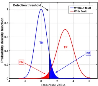
To evaluate whether the residual value indicates a faulty case or not, a threshold value has to be determined, indicating the limit between faulty and normal case. To that end, a Receiver Operating Characteristics (ROC) graph has been used. ROC graphs are useful for characterizing and visualizing the performance of a detection algorithm [38]. The principle of the method is given below. To account both for model uncertainties and measurement noise, the residuals have to be characterized by their probability density functions under the hypotheses of “fault” and “no fault”, as sketched for one residual in Figure 2. The blue curve represents the
probability density function in nominal operating conditions, whereas the orange one represents a faulty case. It can be seen that the supports of the two probability density functions (pdf) are not completely disjoint, leading to possible false decisions. Thus, to decide whether there is a fault or not, a threshold, represented by a black line, is used. The algorithm detects a fault when the absolute value of the residual is higher than the threshold value. The probability to detect correctly a fault is represented by the area below the pdf and above the threshold, noted TP or “True Positive” probability. However, above the threshold, there is also a part of the blue curve (i.e. the residual pdf for nominal conditions) that is non-zero, which leads to False Positive decisions, and the blue area represents the “False Positive” probability (FP). Similarly, below the threshold, the algorithm does not detect a fault. If there is indeed no fault, this leads to a “True Negative” event (TN) whose probability is given by the area under the blue pdf and below the threshold value. Otherwise, it is a False Negative (FN) event whose probability is represented by the orange area. Based on these probabilities, a ROC curve can be plotted (Figure 3). The ROC curve plots parametrically true positive probability (TP) versus false positive probability (FP) with threshold as a varying parameter [39]. The Area Under Curve (AUC) is computed to assess the efficiency of the detection. The best possible detection method would yield a point in the upper left corner or coordinate (0,1) of the ROC space, representing no false negatives and 100% true positives. A random guess would give a point along a diagonal line. Based on these considerations, it is thus possible (i) to assess the quality of a residual for fault detection purposes and (ii) to adjust the threshold values in order to obtain trade-off between benefits (true positives) and costs (false positives).
2.1.4 Isolation step
Once defaults are detected, they are isolated by a supervised classifier. The k Nearest Neighbours classifier (k-NN) [40] is chosen for several reasons. The first one is that in the residual space, the separations between classes are non-linear. Secondly, assumptions on the
repartition probability of the points in the residual space are difficult to make. Finally, k-NN algorithm is easy to implement because there is only one integer parameter (k) to set. The approach [41] achieves the classification goal by creating a residual space, with r2 on x-axis and
r1 on y-axis. All the training data are represented in this space. When a new data has to be
classified, the distances to all the training data are computed. Then, the k nearest instances are selected and the class that have the most instances in this group is chosen as the class of the new data. To be relevant, the database must be representative of all possible faults. To that end, it would have been possible to use part of the experimental measurements. But in that case, it would imply having sufficient data, which may not be relevant for on-line diagnosis. Moreover, the model would no more be used. Therefore, we have chosen to build the training database by simulating the model at different operating conditions. Consequently, the test date set, that is experimental data are completely different from the training data set, based on simulation, ensuring a strong evaluation of the procedure performance, and thus validating the method relevancy.The training data are labelled with faulty operating conditions as in Eq. 2:
𝑟(%)*'$&' = -𝑂
(%)*'$&' − 𝑂+$&'/ (2)
where 𝑂(%)*'$&' is the model output estimated in faulty conditions and 𝑂
+$&' the model output estimated in nominal conditions.
2.2 Experimentation and model 2.2.1 Experimentation
A PEM fuel cell stack designed for automotive application is used. The stack, based on stamped metallic bipolar plate, is composed of 20 cells with an active surface area of 220 cm². A test bench (Figure 4) is used to control precisely operating conditions during experiments such as humidity, stoichiometry, pressure and temperature. Impedance measurements are made using a commercial potentiostat (Autolab 302N form Ecochemie).
Considered faults
The nominal and abnormal operating conditions, considered as faults, are defined in Table 1. The five faulty operating conditions come from three sources:
(i) Stack temperature decrease.
(ii) Relative humidity of gases at the stack inlets (RH). A decrease leads to membrane drying whereas an increase to flooding. The relative humidity is supposed to be the same at the anode and cathode.
Partial pressure of reactive gases (P), with two cases (decrease or increase). This fault corresponds to either a change in stoichiometry at the anode (Sta) or at the cathode (Stc).
2.2.2 Data base at beginning of life
The new fuel cell stack was first characterized by polarisation curves and broad-range impedance spectroscopy for normal and faulty operating conditions. For polarisation characterisations, the current density range is from 0 to 0.85 A.cm-2, insuring cell voltage above 0.5V. EIS characterizations were carried out using an excitation sinusoidal current with amplitude variation of 10% around the DC current value. The frequency range was from 0.02Hz to 1kHz. Figure 5 shows Nyquist diagrams for three different relative humidity contents (RH), for a current density of 0.5 A.cm-2. The high frequency resistance Rhf meas is the impedance value measured when its imaginary part is zero. In the figure, one can verify that its value is sensitive to relative humidity variations, and that its value decreases when the relative humidity content (RH) increases: around 97 mΩ∙cm2.cell-1 for HR=25%, and 89 mΩ∙cm2.cell-1 for HR=50%. These measurements have been used for model parameter tuning and model
validation. In order to obtain a database to evaluate the diagnostics algorithm performances, these experiments have been repeated with different operating conditions. The mean stack voltage and the high frequency resistance have been measured for three DC current density values: 0.25, 0.5 and 0.65 A.cm-2 and each abnormal operating condition.
2.2.3 Experimental database on ageing stack
Fuel cell ageing is carried out through endurance testing by applying FD-DLC (Fuel cell Dynamic Load Cycle), which characterises the demand in current of a driving car. Each cycle is 1180s long, that is about 20 minutes. The 800 first seconds correspond to urban usage whereas the last 380 seconds to extra-urban usage as shown in Figure 6(a). The mean cell voltage response is given in Figure 6(b). The fuel cell was degraded by applying FD-DLC cycles during 1,000h with a current range from 0 to 1 A.cm-2 [35,42]. The resulting mean cell voltage is shown in Figure 7. During the first 100h, one can see the effect on voltage of the characterisations that have been previously conducted, which corresponds to the “beginning of life”. After this period, four ageing phases have been carried out and polarisation curves and EIS characterizations have been performed at the end of each one (300h, 600h, 800h and 1,000h). For each one, the mean stack voltage and the high frequency resistance have been measured for three DC current density values (0.25, 0.5 and 0.65 A.cm-2) and normal and abnormal operating conditions.
2.2.4 Model equations and validation at beginning of life Model equations
The MEPHYSTO-FC model [12,35] is designed as follows. A main modelling hypothesis is to consider all the phenomena in the different cells are identical. The model is constituted of a set of transport and balance equations (mass and enthalpy balance are solved in each nodes) of the channels, GDL, and membrane. In the GDL, the transport equations are based on Maxwell-Stefan equations for the gases and adding the formalism from [43] and Darcy equations for liquid water. Inside the membrane, the equations of water transport are based on diffusion and
electro-osmosis mechanisms. Thermal aspects are also considered by solving enthalpy balances in each node in all the domains of the stack (bipolar plate, MEA, cooling circuit, terminal plate). From these equations, the electrochemical response of a cell to dynamic operating conditions
can be determined. The voltage Uest is computed from the system of equation Eq. 3, derived
from a semi-empirical relation issued from the Butler-Volmer equation [12,35]. The current on each cell (I) is the sum of the currents on each mesh (im). It is assumed to be equipotential along the surface of the cell, it means the voltage value is the same for all the meshes.
0 𝐼 = 2 𝑖# ∀𝑚, 𝑈$&' = (𝑈 ,$- )#+ 𝜂#− (𝑅/0#)#⋅ 𝑖# (3) With 𝜂# = 2(𝑋#)1⋅ β1 2 13! and 𝑋!= #1 𝑇! 𝑇!⋅ 𝑙𝑛 ) 𝑖! 𝐸𝐶𝑆𝐴!/ 𝑇!⋅ 𝑙𝑛 11 𝑃"∗! 𝑃$3 ! 3 𝑇!⋅ 𝑙𝑛 11 𝑃%∗! 𝑃$3 ! 3 𝑇!⋅ 𝑙𝑛 11 𝑃%∗!" 𝑃$ 3 ! 3 𝑖! 𝐸𝐶𝑆𝐴! 𝜎! 5
Where the subscript m indicates that it is the local value on the mesh, 𝑈$&' is the cell potential (V), Urev is the reversible cell potential from the thermodynamic equilibrium (V), η is the overpotential (V) with η≤ 0, Rohm is the specific ohmic resistance of the cell (Ω.m2), T is the local temperature (K), 𝑃1∗ is the partial pressure of the species k (O
2, H2 or H2O) at the active layer interface (Pa), P0 is the standard pressure (Pa), I is the current (A), ECSA the ElectroChemical Surface Area (m2), σ is the protonic conductivity of the active layer (S.m-1). βk are semi-empirical coefficients (V or V.K-1 or m).
The values of these parameters are computed by the model, except the β1 parameters which
have to be tuned. To determine the value of the high frequency resistance, Uest is calculated first by the model, using the same excitation current signal as in experimentations. Then, the
amplitude (ΔU) of the signal Uest is computed using Fast Fourier Transform (FFT). Thus, the high frequency resistance is:
𝑅ℎ𝑓$&' = ?𝛥𝑈
𝛥𝐼A (4)
Model validation
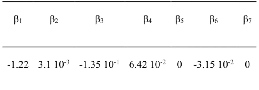
Polarisation curves measured on the new stack are used to fit the βk model parameters of the
fuel cell stack. The method used to fit the parameters is detailed in [35] and the estimated parameter values are listed in Table 2. Polarisation curves from model simulation and experimental measurements with different operating conditions are shown in Figure 8(a). It can be seen that the model closely matches experimental data at beginning of life. As a mean error of 5 mV.cell-1 and a standard deviation of 5 mV.cell-1 are obtained, the model is considered to be validated. In order to validate the ability of the model to estimate high frequency resistance, experimental and model resistances are compared for different operating conditions. In Figure 8(b) are plotted the experimental high frequency resistances against those obtained from the model. Nominal conditions are represented with green crosses and the faulty conditions by in red circles. The results show a mean difference of 0.003 Ω∙cm2.cell-1 with a standard deviation of 0.0065 Ω∙cm2.cell-1. Thus, the model can be used to estimate high frequency resistances.
2.2.5 Model adaptation and validation for ageing stack
The degradation of the fuel cell is modelled in order to predict the evolution of Uest during
ageing, using [44] as a reference. The idea is to replace the local ElectroChemical Surface Area (ECSAm) in eq. 3 by a degradation rate τdegr,m of platinum dissolution depending on time. The
new expressions of Xm(3) and Xm(7) of the model becomes then:
𝑋#(3,7) = D𝑇#𝑙𝑛 D 𝑖#
𝐸𝐶𝑆𝐴_𝑖𝑛𝑖 . 𝜏7$8,,#O ,
𝑖#
𝜎#⋅ 𝐸𝑆𝐶𝐴_𝑖𝑛𝑖. 𝜏7$8,,#O
(5)
τdegr= ECSA(t) ECSA_ini
(6) With ECSA(t) the surface area at time t and ECSA_ini the surface area at the beginning of life. To evaluate the evolution of ECSA(t) with respect to time, a law, taken from [44], dependant on dissolution speed with particle size, temperature, potential, oxygen and vapor partial pressures is used and given below:
Y 𝐸𝐶𝑆𝐴(𝑡) = 𝐸𝐶𝑆𝐴=+=− [ 𝜈7=&& ' > ν?@AA= k ⋅ e B! CD(FG&HFG'(')HFG*'+ ) (7) Where 𝜈7=&& is the dissolution speed, k is the direct reaction constant (𝑚𝑜𝑙 ⋅ 𝑚B"⋅ 𝑠B!), R the perfect gas constant (J.mol-1.K-1), T the temperature (K), ΔG
J is the variation of free enthalpy required for a platinum atom extraction (J) calculated by Discrete Fourier Transform (DFT).
ΔGKLKM = −2𝛼𝐹Δ𝜒 is the variation of free enthalpy required for a platinum atom oxidation (J)
with 𝛼 the transfer coefficient, F the Faraday constant (C.mol-1) and Δ𝜒 the local potential in the inner layer (V). ΔG?KA = −𝛽 𝐸NO(𝑟P') is the variation of free enthalpy required for leaching of Pt2+ (J) with 𝐸
NO the Gibbs Thomson energy that depends on the radius of the platinum
particle.
After the adjustment of the parameters of the degradation rate (distribution of platinum particles, initial radius of platinum particles), the validity of the model during aging is tested by the evaluation of the maximum power delivered by the stack. Figure 9 shows this experimental power and the model estimation during ageing. The decrease of the power is globally properly described by the degradation laws, although it is underestimated at the end.
3 Results and Discussion
3.1 Results for a fuel cell at beginning of life
In this part, the diagnosis methodology described in part 2 is applied.
3.1.1 ROC curves
The validated MEPHYSTO-FC model is now run with the three DC current density values:
0.25, 0.5 and 0.65 A.cm-2, in nominal operating conditions. Thus, the estimated mean voltage
and high frequency resistances are i𝑈$&' 𝑅ℎ𝑓$&'j = 𝑓(𝐼#$%&; 𝑇+; 𝑅𝐻+; 𝑃+; 𝑆𝑡
%+; 𝑆𝑡Q+)
where exponent est, and meas refer to estimated, nominal and measured respectively, and
subscripts and refer respectively to the anode and cathode.The residuals r1 and r2 are
defined as the difference between the measured values and the estimated ones (Equation 1): 𝑟 = $𝑟𝑟!
"% = &
𝑈#$%&− 𝑈$&' 𝑅ℎ𝑓 #$%&− 𝑅ℎ𝑓 $&',
where the measurements are issued from the experimental database taken at the beginning of the stack life (section 3.2).
In order to assess the detection performances, two ROC curves are built, one with the residual r1 and the other with the residual r2. In Figure 10a, the ROC curve is plotted for the residual r1. As can be seen from the graph, good detection performances can be expected, that is confirmed by the fact that the Area Under Curve (AUC) is equal to 0.93. The range of threshold values has been taken from 1.6 mV.cell-1 to 50 mV.cell-1. It can be noted that the curve rises vertically from the threshold value of 50 mV.cell-1 to 10 mV.cell-1, indicating that there is no probability of false alarm, for the analysed experiment. Then the direction of the curve changes by taking a slight slope up to the threshold value of 1.6 mV.cell-1 for which no fault would be detected. Thus, the optimal threshold value of 10 mV.cell-1, which corresponds to the case for which the probability of detection is the highest while having no probability of false alarm, is chosen. The ROC curve is now plotted for the second residual r2 in Figure 10b. The Area Under Curve
n
(AUC) is 0.89, showing a good detection performance. The threshold is chosen at 8.8 mΩ∙cm2.cell-1 in order to minimise the false positive probability.
3.1.2 Fault detection results
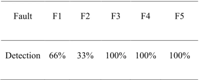
With the threshold values fixed previously, the probabilities of true detection for each faulty
condition and based on the residual r1 are shown in Table 3. It can be seen that some of the
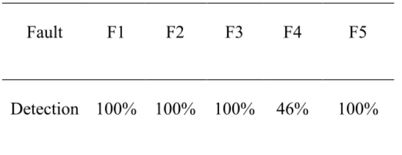
faults are perfectly detected, such as pressure modifications (F4, F5) and a decrease of the inlet humidity (F3). However, the faults that induce a flooding (F1, F2) are poorly detected. This can be explained by the fact that flooding has a weak impact on the stack voltage, and the residual r1 is thus not sensitive to these faults. Similarly, the probabilities of true detection for each faulty condition based on the residual r2 are shown in Table 4. For this residual, faults relating to humidity inlet and change of temperature (F1, F2 and F3) are perfectly detected, as well as F5, relating to an increase of partial pressure. However, the fault F4, relating to a decrease of partial pressure, is poorly detected. Consequently, none of the residuals can detect all the faults alone. But, considering both residuals together, the algorithm is able to detect 100% of the faults without any false alarm.
3.1.3 Classifier training
The chosen method to isolate the detected faults is the k-NN classifier. To implement it, the first step is to generate a training database. As detailed in section 2.4, residuals were generated by replacing experimental measurements with model simulations in faulty operating conditions for three density current values (0.25 ; 0.5 and 0.65 A.cm-2). The advantage of proceeding this way is there is no need to have large amounts of data or to embed the model. Additionally, since the experimental data will be only used to assess the fault isolation performances, this approach will allow validating the method relevancy. Then, the estimated residuals 𝑟(%)*'$&' were labelled with the five faulty operating conditions (F1 to F5) considered in our study. To be as close as possible from reality cases, the operating conditions are varied from the nominal conditions to the faulty operating conditions. For example, the fault F1 will take 10 temperature values,
beginning from 80°C to 60°C in steps of 2°C, so that faults can be isolated over a large validation domain. Consequently, 46 different operating conditions labelled with the five faults are thus considered that are detailed in Table 5. The resulting training data set is presented in the residual plane shown in Figure 11. In this figure, the residuals r2 are represented on the x-axis and the residuals r1 on the y-axis, so each estimated residuals 𝑟(%)*'$&' of the database is represented by a point in the plane. The origin of the axes, the point (0,0) corresponds to the nominal case. The white rectangle represents the cases that are under the thresholds, thus the residuals that are inside this area are not detected as faults. The k-NN algorithm is then trained with the detected residuals to define the classification rules, which are represented by the coloured areas.
3.1.4 Fault isolation results on real measurements
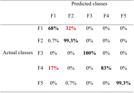
Once trained on simulated data, the k-NN algorithm can be used to classify the experimental points obtained from real measurements ; its performance can then be assessed with a test data set (based on real measurements) completely different from the training set (based on simulation), which guarantees a sound performance evaluation procedure for the proposed classifier. The resulting residual plane is shown in Figure 12. In this figure, the points corresponding to the nominal operating conditions are marked with green asterisks and are as expected in the non-detected area. It can be noticed that there is neither false alarm nor missed detection. As intended, the detection algorithm detects all the faults. Concerning fault isolation, it can be seen that the faults F3 and F5 are properly isolated, whereas the other faults, that are F1, F2 and F4, are not perfectly classified. To go further, the confusion matrix of the classifier is shown in Table 6. In this table, the columns represent the predicted or estimated classes whereas the rows represent the actual classes. All correct predictions are located in the diagonal of the table (highlighted in bold), so the prediction errors are represented by values outside the diagonal. The confusion matrix shows three very high levels of isolation. Indeed, F2, F3 and F5 are correctly classified on more than 99% of the data. However, F1 and F4 are not so well
isolated, with only 68% of isolation for F1 and 83% for F4. This means for the fault F4, which corresponds to the decrease of partial pressures, that 17% are classified as F1, which corresponds to temperature decrease. Similarly, for the data belonging to F1, 32% of the data are mistakenly classified as F2. This last confusion can be explained with a physical interpretation. In fact, both operating conditions (decrease of temperature and an increase in relative humidity of inlet gases) will induce flooding inside the cell. Therefore, the confusion between the two faults does not necessary be avoidable and the corrective action taken by the controller is expected to decrease flooding. At last, the global isolation average score is 91%, which can be thus considered as reliable.
3.2 Results for the aged fuel cell
3.2.1 Adaptation of the method to ageing
The diagnostic method can now be tested with experimental measurements of aged fuel cell stack. The classification results obtained at 300h without ageing modelling are shown in Figure 13. It can be seen that the residuals (even those obtained with the nominal operating conditions) all lie outside the nominal condition zone, which leads to the decision “fault detected” in each case, i.e. the probability of false alarm is 100%. In other words, this means that ageing modifies the fuel cell performances and that the model is thus no longer accurate enough for a correct detection. Thus, it is necessary to adapt the method. The model used is now the modified model for ageing stack and that includes the degradation rate tdegr, time-dependent value. The estimated mean voltage and high frequency resistances are computed with the adapted model for the three different DC current density values: 0.25, 0.5 and 0.65 A.cm-2, with nominal operating conditions. The measured mean voltage and high frequency resistances are taken from the entire experimental database, that is nominal and faulty operating conditions as well as at all ageing stages (beginning of life, 300h, 600h, 800h and 1,000h). Then, the new detection performances have to be characterized again and are thus visualized with ROC curves for both residuals r1 and r2. The ROC curve for the residual r1 is shown in Figure 14a. The Area Under
Curve (AUC) is now 0.75, which is lower than 0.93 at beginning of life. It can be seen on the figure that keeping the threshold value at 10mV will lead to 10% of false alarms. It is thus no longer appropriate and a value of 11mV seems more suitable, which decreases the number of false alarms to 5%. However, by doing this, the probability of true fault detection is reduced by
3%, from 54% to 51%. The ROC curve for the residual r2 is shown in Figure 14b. This time the
Area Under Curve (AUC) remains high with the value 0.93, showing that the detection still stands very good. Additionally, the threshold value can be kept at 8.8 mΩ∙cm2.cell-1, value that minimises the false positive probability, but with a detection score of 46% only. This detection score may be increased to 67% by choosing a threshold value of 5 mΩ∙cm2.cell-1, but this would induce some false alarms (2.5%). Finally, thresholds were reassessed at 11mV.cell-1 for r1 and kept at 8.8 mΩ∙cm2.cell-1 for r
2.
3.2.2 Detection results
With the previous threshold values, the detection algorithm is applied during ageing and the resulting detection performances are detailed in Table 7. It can be seen that during the entire lifetime of the fuel cell, the probability of false alarm is only 5%. Looking further at different stack ageing, there is no false alarm except at 1000h, where it raises to 33%. This can be interpreted by considering that the model is no more valid even under nominal conditions. It can be seen for the case with all experiments that the true detection probability is 100% for F3 and F5, but only 61% for F1 and 44% for F2. The probability of the algorithm to miss the detection of these faults is high. These performances could be easily improved by changing the threshold of r2 to 5mΩ∙cm2.cell-1. Then, the new probabilities of true detection would be 67% for F1 and 81% for F2. However, performance improvement is not only a threshold level issue and the way to improve the algorithm can be discussed. The first thing to do would be to exploit the fact that voltage and high frequency resistance are not independent and use it for fault detection. Another way would be to improve the model accuracy so as to enhance detection performances and thus to reduce the probability of missed detection. Finally, considering that
the chosen indicators, i.e. voltage and high frequency resistance, are not sufficiently sensitive to faults F1 and F2, new features may also be found. However, the purpose of this study is to explore a new methodology, and in that way the results are sufficient to validate the relevancy of the approach.
3.2.3 Isolation
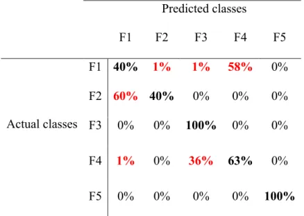
The detected faults are now isolated thanks to the same k-NN classifier used at the stack beginning of life. The resulting residual plane is shown in Figure 15. It should be noted that the nominal case as well as some faults F1 and F2 are in the non-detected area, which is consistent with the detection results. Moreover, as for the beginning of stack life, the classifier correctly identifies the faults F3 and F5, but not F1, F2 and F4. More precise results are shown in Table 8, which represents the confusion matrix obtained for the entire data. The results shown in Table 8 are consistent with those at beginning of life (Table 6). It can be seen that faults F3 and F5 are again properly isolated with a high-level score. The F1 and F4 faults, which had previously the worst isolation scores, have now an even worse score compared with the beginning of life (true positive from 68% to 40% for F1 and 83% to 63% for F4). Moreover, the F2 fault is also poorly isolated with a true positive score of 40%. Thus, the table highlights three confusions on fault isolation: F1 considered as F4 fault, F2 as F1 and F4 as F3. However, confusion between the faults F2 and F1 was already present at the beginning of the stack life, and as both will induce flooding inside the cell, this does not necessary have to be avoided. However, the two other confusions, F1 taken for F4 and F4 taken for F3, are more inconvenient and a wrong decision on the stack may worsen the fault.
4 Conclusions
In this work, a model-based methodology for fault detection and isolation robust to dynamic operating conditions and stack ageing was proposed. The methodology is divided into three steps (residual generation, fault detection and fault isolation) which have been developed first
for fuel cell at beginning of life and then adapted for ageing fuel cell. Performances were estimated for five abnormal operating conditions considered as faults thanks to experimentations that were carried out during 1,000h, with periodically characterisations in abnormal operating conditions. Following the model-based fault detection method, the MEPHYSTO-FC model is used to compute the residuals based on voltage and high frequency resistance. At the fuel cell’s beginning of life, the ROC curves allowed setting the thresholds so that there is no false alarm. The results on the detection probabilities show that faults F1, F2 and F4 are the least well detected and that the two residues must be used to obtain 100% detection. These detected faults are then isolated by the classifier. The results gives that no false alarm occurs and fault isolation is perfect (100%) except for F1 (68%) and F4 (83%). During ageing, experimental results show that without any adaptation, detection drops dramatically to 0% right from 300h. Consequently, the model is used with ageing mechanisms and the thresholds are adjusted. Thanks to these improvements, probability of false alarm remains globally very low (5%). Faults F3 and F5 were properly detected and isolated during the whole life of the stack. Fault F4 was detected on 86% of the whole data and properly isolated in more than 60% of the detected cases. However, faults F1 and F2 were poorly diagnosed with large confusion between these faults. However, this confusion can be physically explained. The other confusions (F1 taken for F4 and F4 taken for F3) have to be avoided, and to that aim, two kinds of research could be developed, that are model improvement and new indicators seeking. Notwithstanding these points of improvement, this method has however proved its robustness towards ageing and it can be concluded that the proposed approach is reliable for fault detection and isolation in dynamical and ageing conditions.
References
[1] T. Ous, C. Arcoumanis, J. Power Sources, 2013, 240, 558. [2] T. Zhang, P. Wang, H. Chen, P. Pei, Appl. Energy, 2018, 223, 249. [3] W. Schmittinger, A. Vahidi, J. Power Sources,2008, 180, 1, 1.
[4] N. Yousfi-Steiner, P. Moçotéguy, D. Candusso, D. Hissel, A. Hernandez, and A. Aslanides, J. Power Sources, 2008, 183, 1, 260.
[5] N. Yousfi-Steiner, P. Moçotéguy, D. Candusso and D. Hissel, J. Power Sources, 2009,
194, 1,130.
[6] A. Benmouna, M. Becherif, D. Depernet and F. Gustin, Int. J. Hydrogen Energy, 2017,
42,2, 1534.
[7] R. Salim, H. Noura and A. Fardoun, Conference on Control and Fault-Tolerant Systems
(SysTol), 2013, Nice, October 9-11.
[8] R. Petrone, Z. Zheng, D. Hissel, M. Péra, C. Pianese, M. Sorrentino, M. Becherif and N. Yousfi-Steiner, Int. J. Hydrogen Energy, 2013, 38, 17, 7077.
[9] A. Rosich, R. Sarrate et F. Nejjari, Appl. Math. Model., 2014, 38, 2744.
[10] J. Liu, W. Luo, X. Yang and L. Wu, IEEE Trans. Ind. Electron., 2016, 63, 5, 3261. [11] P. Polverino, E. Frisk, D. Jung, M. Krysander and C. Pianese, J. Power Sources, 2017,
357, 26.
[12] C. Robin, M. Gerard, M. Quinaud, J. d Arbigny et Y. Bultel, J. Power Sources, 2015,
326, 417.
[13] Z. Zheng, R. Petrone, M. Péra, D. Hissel, M. Becherif, C. Pianese, N. Yousfi Steiner and M. Sorrentino, Int. J. Hydrogen Energy, 2013, 38, 21, 8914.
[14] H. Lu, J. Chen, C. Yan and L. H., J. Power Sources, 2019, 430, 233.
[15] M. Stepančič, D. Juričić et P. Boškoski, Energ Convers Manage., 2019, 195, 76. [16] J. Liu, Q. Li, W. Chen, Y. Yan and X. Wang, IEEE Trans. Transport. Electrific., 2016,
5, 1, 271.
[17] Z. Li, R. Outbib, D. Hissel and S. Giurgea, Control Eng. Pract., 2014, 28, 1.
[18] E. Pahon, N. Yousfi Steiner, S. Jemei, D. Hissel and P. Moçoteguy, Appl. Energy, 2016,
165, 748.
[19] R. Petrone, E. Pahon, F. Harel, S. Jemei, D. Chamagne, D. Hissel and M. Pera, IEEE
Vehicle Power and Propulsion Conference, VPPC 2017, 2017, Belfort, France,
december 11-14.
[20] P. Pei, Y. Li, H. Xu and Z. Wu, Appl. Energy, 2016, 173, 366.
[21] Z. Li, C. Cadet and R. Outbib, IEEE Trans. Energy Convers., 2019, 34, 2, 964.
[22] G. Mousa, F. Golnaraghi, J. DeVaal and A. Young, J. Power Sources, 2014, 246, 110. [23] S. Tant, S. Rosini, P.-X. Thivel, F. Druart, A. Rakotondrainibe, T. Geneston and Y.
Bultel, Electrochim. Acta, 2014, 135, 368.
[24] S. Labiri, K. Mammar, M. Hamouda and Y. Sahli, Int. J. Hydrogen Energy, 2016, 41,38, 17093.
[25] P. Ren, P. Pei, Y. Lia, Z. Wua, D. Chena and S. Huanga, Appl. Energy, 2019, 239, 785. [26] N. Fouquet, C. Doulet, C. Nouillant, G. G. Dauphin-Tanguy and B. Ould-Bouamama, J.
Power Sources, 2006, 159, 905.
[27] A. Hernandez and D. Hissel, IEEE Trans. Energy Convers., 2010, 25, 1, 148. [28] S. Rezaei Niya and M. Hoorfar, J. Power Sources, 2013, 240, 281.
[29] Z. Zheng, M. Pera, D. Hissel, M. Becherif, K. Agbli et Y. Li, J. Power Sources, 2014,
271, 570.
[30] A. Miege, F. Steffen, T. Luschtinetz, S. Jakubith and M. Freitag, Energy Procedia, 2012,
[31] I. Halvorsen, I. Pivac, I. Bezmalinović, F. Barbir and F. Zenith, Int. J. Hydrogen Energy,
2020, 45, 2, 1325.
[32] D. Ritzberger, M. Striednig, C. Simon, C. Hametner and S. Jakubek, J. Power Sources,
2018, 405, 150.
[33] C. Jeppesen, S. Araya, S. Sahlin, S. Thomas, S. Andreasen and S. Kær, J. Power Sources,
2017, 359,.37.
[34] R. Onanena, L. Oukhellou, D. Candusso, A. Same, D. Hissel and D. Aknin, Int. J.
Hydrogen Energy, 2010, 35, 15, 8022.
[35] C. Robin, M. Gerard, J. d'Arbigny, P. Schott, L. Jabbour and Y. Bultel, Int. J. Hydrogen
Energy, 2015, 40, 32, 10211.
[36] K. Tidriri, N. Chatti, S. Verron and T. Tiplica, Annu Rev Control., 2016, 42, pp.63. [37] R. Isermann, Fault-diagnosis systems - an introduction from fault detection to fault
tolerance, Springer, 2006.
[38] T. Fawcett, Pattern Recognit. Lett., 2006, 27,.861.
[39] H. Van Trees, K. Bell and Z. Tian (with), Detection Estimation and Modulation Theory,
Part I: Detection, Estimation, and Filtering Theory, 2nd Edition, New York Chichester:
Wiley, April 2013.
[40] C. Bishop, Pattern Recognition and Machine Learning, Springer, 2006. [41] N. Altman, Am Stat, 1992, 46, 3, 175.
[42] G. Tsotridis, A. Pilenga, G. De Marco et T. Malkow, EU Harmonised Test Protocols for PEMFC MEA Testing in Single Cell Configuration for Automotive Applications, JRC
Science for Policy report, EUR 27632 EN, 2015.
[43] J. Young, B. Todd, Int. J. Heat Mass Transf., 2005, 48, 125-26, 5338.
Figure Captions
Figure 1: Diagnosis method
Figure 2 : Probability density function of a residual under nominal and faulty condition Figure 3 : ROC curve - True positive probability against false positive probability for
different threshold values
Figure 4: Fuel cell test stack on the test bench
Figure 5: EIS at 0.5A.cm-2 for nominal and faulty relative humidity values
Figure 6 : FD-DLC cycle applied to the stack (a) Driving current demand (b) Mean voltage response
Figure 7 : Mean cell voltage during the 1000h-long experiment and characterization times Figure 8: Validation of the model: (a) polarization curves during faults F4, F5 and nominal
conditions at beginning of life (b) comparison between model and experimental high frequency resistances
Figure 9 : Validation of the aging dependency of the model
Figure 10: ROC curve - Performance of residuals to detect faulty conditions based on (a) the first residual r1 and (b) the second residual r2
Figure 11 : Training data and classification areas
Figure 12: Detection residual space and residuals obtained during the experiments Figure 13: Isolation without ageing modelling at 300h
Figure 14 : ROC curve with aged data (a) the first residual r1 and (b) the second residual r2 Figure 15 : Isolation results for all data
Table Captions
Table 1. Nominal and faulty operating conditions Table 2. Electrochemical parameters of the model
Table 3. Detection probabilities based on the residual r1 for each faulty condition Table 4. Detection probabilities based on the residual r2 for each faulty condition Table 5. Operating conditions of training data
Table 6. Confusion Matrix : fault isolation results
Table 7. Detection probabilities during ageing (r1=11mV.cell-1; r2=8.8 mΩ∙cm2.cell-1) Table 8. Confusion Matrix for the aged data
Table 1 Nominal and faulty operating conditions.
Fault Name Faulty Operating Conditions
Nominal: T=80° C, RH=50%, P=1.5 105 Pa, Sta = 1.5, Stc = 2
F1 Temperature decrease T=60°C
F2 Flooding RH=75%
F3 Drying RH=25%
F4 Partial Pressure decrease P=1.2 10
5 Pa, St
a = 1.2 P=1.2 105 Pa, Stc = 1.5
F5 Partial Pressure increase P=2.5 10
5 Pa, St a = 2 P=2.5 105 Pa, Stc = 2.5
Table 2. Electrochemical parameters of the model
β1 β2 β3 β4 β5 β6 β7
Table 3. Detection probabilities based on the residual r1 for each faulty condition
Fault F1 F2 F3 F4 F5
Table 4. Detection probabilities based on the residual r2 for each faulty condition
Fault F1 F2 F3 F4 F5
Table 5. Operating conditions of training data
Fault Faulty value Operating conditions interval Step
F1 T = 80°C T = [60°C ; 80°C] 2°C F2 RH = 75% RH = [50% ; 80%] 5% F3 RH = 25% RH = [20% ; 50%] 5% F4 Sta = 1.2 Stc = 1.5 Sta = [1.2 ; 1.5] Stc = [1.5 ; 2] 0.05 F5 Sta = 2 Stc = 2.5 Sta = [1.5 ; 1.2] Stc = [2 ; 2.5] 0.05
Table 6. Confusion Matrix : fault isolation results Predicted classes F1 F2 F3 F4 F5 Actual classes F1 68% 32% 0% 0% 0% F2 0.7% 99.3% 0% 0% 0% F3 0% 0% 100% 0% 0% F4 17% 0% 0% 83% 0% F5 0% 0.7% 0% 0% 99.3%
Table 7. Detection probabilities during ageing (r1=11mV.cell-1; r2=8.8 mΩ∙cm2.cell-1) Nominal F1 F2 F3 F4 F5 All 95% 61% 44% 100% 86% 100% 0h 100% 79% 100% 100% 100% 100% 300h 100% 45% 33% 100% 50% 100% 600h 100% 67% 29% 100% 100% 100% 800h 100% 61% 32% 100% 100% 100% 1,000h 67% - 33% 100% 100% 100%
Table 8. Confusion Matrix for the aged data Predicted classes F1 F2 F3 F4 F5 Actual classes F1 40% 1% 1% 58% 0% F2 60% 40% 0% 0% 0% F3 0% 0% 100% 0% 0% F4 1% 0% 36% 63% 0% F5 0% 0% 0% 0% 100%
Figure 2 - Probability density function of a residual under nominal and faulty condition -4 -2 0 2 4 6 Residual value 0 0.2 0.4 0.6 0.8 1
Probability density function
Without fault With fault TN TP FN FP Detection threshold
Figure 3 - ROC curve - True positive probability against false positive probability for
different threshold values
0 0.1 0.2 0.3 0.4 0.5 0.6 0.7 0.8 0.9 1
False positive rate
0 0.2 0.4 0.6 0.8 1 1.2
Figure 5 - EIS at 0.5A.cm-2 for nominal and faulty relative humidity values
0 0.1 0.2 0.3 0.4 0.5 0.6 0.7
Real part of impedance / cm2cell-1
-0.15 -0.1 -0.05 0 0.05 0.1 0.15 0.2 0.25 0.3
Imaginary part of impedance /
cm 2 cell -1 Nominal F2HR=75% F 3HR=25% 0.08 0.1 0.12 0.01 0.02 0.03
Figure 6 - FD-DLC cycle applied to the stack (a) Driving current demand (b) Mean voltage response 0 200 400 600 800 1000 1200 Time / s 0 0.2 0.4 0.6 0.8 1 Current density / A cm -2 Urban Extra-urban a) 0 200 400 600 800 1000 1200 Time / s 0.6 0.7 0.8 0.9 1 Mean voltage / V Voltage at OCV b)
Figure 8 - Validation of the model: (a) polarization curves during faults F4, F5 and nominal
conditions at beginning of life (b) comparison between model and experimental high frequency resistances 0 0.2 0.4 0.6 0.8 1 Current Density / A cm-2 0.5 0.55 0.6 0.65 0.7 0.75 0.8 0.85 0.9 0.95 Cell voltage / V Nominal, experiment Nominal, modeled F4, experiment F4, modeled F5, experiment F5, modeled a) 0.08 0.1 0.12 0.14
Model high frequency resistance / cm2cell-1
0.07 0.08 0.09 0.1 0.11 0.12 0.13 0.14 0.15 E xper imenta l h igh frequency resistance / cm 2 cell -1 Nominal F1T=60°C F2RH=75% F3RH=25% F4P=1.2 105Pa F5P=2.5 105Pa y=x 15%error
b)
Figure 9 - Validation of the aging dependency of the model 0 200 400 600 800 1000 1200 1400 Ageing time / h 0.52 0.54 0.56 0.58 0.6 0.62 0.64 Maximum power P max / W cm -2 Experimental values Model estimation
Figure 10 - ROC curve - Performance of residuals to detect faulty conditions based on (a) the
first residual r1 and (b) the second residual r2
0 0.2 0.4 0.6 0.8 1
False positive rate 0 0.2 0.4 0.6 0.8 1
True positive rate
Residual method Random detection Threshold = 10 mV cell-1 Threshold = 50 mV cell-1 Threshold = 1.6 mV cell-1 a) 0 0.2 0.4 0.6 0.8 1
False positive rate 0 0.2 0.4 0.6 0.8 1
True positive rate
Residual method Random detection Threshold = 48 m cm2cell-1 Threshold = 8.8 m cm2cell-1 Threshold = 3 m cm2cell-1 b)
Figure 14 - ROC curve with aged data (a) the first residual r1 and (b) the second residual r2
0 0.2 0.4 0.6 0.8 1
False positive rate 0 0.2 0.4 0.6 0.8 1
True positive rate
Random detection Residual method Threshold = 11 mV Threshold = 10 mV a) 0 0.2 0.4 0.6 0.8 1
False positive rate
0 0.2 0.4 0.6 0.8 1 T rue pos it ive rate Random detection Residual method Threshold = 8.8 m cm2 0.025 Threshold = 5 m cm2 0.46 0.67 b)