HAL Id: hal-03031319
https://hal.archives-ouvertes.fr/hal-03031319
Preprint submitted on 30 Nov 2020
HAL is a multi-disciplinary open access
archive for the deposit and dissemination of sci-entific research documents, whether they are pub-lished or not. The documents may come from teaching and research institutions in France or abroad, or from public or private research centers.
L’archive ouverte pluridisciplinaire HAL, est destinée au dépôt et à la diffusion de documents scientifiques de niveau recherche, publiés ou non, émanant des établissements d’enseignement et de recherche français ou étrangers, des laboratoires publics ou privés.
An MRI-based articulatory characterization of Kannada
coronal consonant contrasts
Alexei Kochetov, Christophe Savariaux, Laurent Lamalle, Camille Noûs,
Pierre Badin
To cite this version:
Alexei Kochetov, Christophe Savariaux, Laurent Lamalle, Camille Noûs, Pierre Badin. An MRI-based articulatory characterization of Kannada coronal consonant contrasts. 2020. �hal-03031319�
1
An MRI-based articulatory characterization of Kannada coronal consonant contrasts
Submitted to
Laboratory Phonology, the Journal of the Association for Laboratory Phonology
Alexei Kochetov
1,2, Christophe Savariaux
2, Laurent Lamalle
3, Camille Noûs
4, Pierre Badin
21 Department of Linguistics, University of Toronto, Toronto, Canada 2 Univ. Grenoble Alpes, CNRS, Grenoble INP, GIPSA-lab, 38000 Grenoble, France
3 Inserm US 17 - CNRS UMS 3552 - Univ. Grenoble Alpes & CHU de Grenoble, UMS IRMaGe, France 4 Cogitamus laboratory
1 Abstract
This paper investigates production mechanisms of a complex set of coronal consonant contrasts in Kannada, with the goals of (i) testing previous theoretical distinctive feature approaches to coronals and (ii) documenting this relatively phonetically under-studied Dravidian language.
An extensive corpus of articulations was collected by static MRI midsagittal from two female speakers, including a full set of Kannada place and manner contrasts in five vowel contexts. Articulatory modelling was used to determine a small set of components responsible for the implementation of various consonant classes, including the place sets of dentals, retroflexes, and alveolopalatals, and manner sets of stops, fricatives, nasals, liquids, and glides. Overlaid average contours were used for the traditional phonetic classification of consonants, while dispersion ellipses were employed to capture consonants’ susceptibility to vowel coarticulation.
The results provide evidence for some of the distinctive feature characterizations of coronals (e.g. constriction location and tongue body height distinctions for dentals and retroflexes), while disconfirming others (tongue dorsum backing for retroflexes). They also largely confirm previous descriptive phonetic accounts of Kannada consonants (including the merger of retroflex and alveolopalatal sibilants), while at the same time identifying somewhat unexpected articulatory patterns (such as dorsal constrictions for /ʋ/, /h/, and /r/).
All the images and articulatory contours are made publicly available.
Keywords
2
2 Introduction
A rapid development of various articulatory methodologies over the last few decades has revolutionised the fields of phonetics and phonology, considerably enriching our understanding of the variation observed in the production of sounds within and across languages. Yet, the majority of articulatory work done so far has focused on a handful of languages, most of which are native to Europe. Thus, among articulatory phonetic studies published in major journals between 2000 and 2019, more than one third focus on English, and more than two thirds focus on Indo-European languages spoken in Europe (with the bulk being major Germanic and Romance languages) (Kochetov, 2020). Given this linguistic bias, it remains to be shown whether empirical findings and theoretical generalizations obtained based on major European languages can extend to a wider range of sound pattern types. As part of our general effort to document articulatory structures of less studied languages, we have developed a static MRI corpus of sounds in Kannada, a Dravidian language spoken in India. Apart from being phonetically under-documented, Kannada is phonologically interesting in having a robust set of coronal phonemic contrasts, with dentals and retroflexes in particular, occurring with various manners of articulation. Articulatory mechanisms involved in the production of retroflexes as well as their phonological representations are topics of an ongoing debate (as reviewed below). An important goal of this work, therefore, is to shed light on the production mechanisms of Kannada consonant contrasts, focusing on coronals of different places and manners of articulation. This is done by employing recent MRI techniques and computational modelling (Labrunie et al., 2018). This work thus aims to add significantly to the insights obtained in recent articulatory research on Kannada retroflexes (Kochetov et al., 2014; Irfana, 2017) and similar contrasts in other related (Narayanan et al., 1999; Scobbie et al., 2013) and unrelated languages (Tabain, 2012; Tabain et al., 2018).
2.1 Coronal consonant contrasts and distinctive features
Coronal place contrasts, such as distinctions between dentals, alveolars, retroflexes, and alveolopalatals, have been a major focus of the distinctive feature theory in phonology for several decades (e.g. Lahiri et al., 1984; Paradis et al., 1991; Hall, 2011). The main goal of this theory is to supply a minimal set of articulatory (or auditory) parameters that (i) distinguishes phonemic contrasts within and across languages and (ii) accounts for respective sounds’ phonological patterning (distribution within a word, alternations with other sounds, etc.). Considering various articulation-based distinctive feature proposals, researchers generally agree that retroflexes are more distinct from dentals than from alveolopalatals (Chomsky et al., 1968; Sagey, 1986; Hamilton, 1996); Gnanadesikan, 1994; Arsenault, 2008). That is, the number of distinctive feature differences is generally greater for the dental-retroflex contrast than for the retroflex-alveolopalatal contrast.
Among the key characteristics noted to distinguish dentals and retroflexes are (i) the location of the constriction along the palate: the binary feature [+anterior] for dentals and [-anterior] for retroflexes (Chomsky et al., 1968; Sagey, 1986; Hall, 1997); the privative features [dental], [postalveolar], [palatal], often combined with underspecification for some of them (Hamilton, 1996; Gnanadesikan, 1994); (ii) the spatial extent of the
3
constriction between the tongue and the roof of the mouth [+distributed] for dentals and [-distributed] for retroflexes (Chomsky et al., 1968; Hall, 1997); (iii) the part of the tongue making the constriction – whether it is the tip, the blade, or the underside ([apical], [laminal], or [sublaminal] (Hamilton, 1996; Gnanadesikan, 1994); (iv) the orientation of the tongue tip ([tip up] for retroflexes and [tip down] for dentals (Gafos, 1999; Hamann, 2003); and (v) the shape of the front portion of the tongue ([tongue middle down] for retroflexes, Hamann, 2003); or [convex] for dentals and [concave] for retroflexes, Arsenault, 2008). Further, some researchers proposed that retroflexes are characterised by (i) a distinct involvement of the posterior portion of the tongue: a backing of the tongue body: features [dorsal] or [back] (Bhat, 1974; Gnanadesikan, 1994; Hamann, 2003; Arsenault, 2008) and (ii) a raising of the tongue dorsum: [high] (Hamann, 2003), as well as (iii) a concomitant lowering of the tongue body for sublaminal retroflexes in particular: [low] (Arsenault, 2008). Finally, retroflexes were noted to be consistently produced with a sublingual cavity, although this is considered to be a consequence of their characteristic tongue tip curling (Hamann, 2003).
Many of the noted features are also relevant for the distinction between retroflexes and alveolopalatals. Specifically, unlike retroflexes, alveolopalatals can be classified as [+distributed] (given their extensive tongue-palate contact: Chomsky et al., 1968; Hall, 1997), [laminal] and [tip down] (given the involvement of the blade and the direction of the tip: Hamilton, 1996; Gnanadesikan, 1994; Gafos, 1999; Hamann, 2003), and [convex] (given the overall shape of the tongue body: Arsenault, 2008). Further, alveolopalatals were noted to be distinguished by a configuration of the posterior portion of the tongue, which could be the reverse of retroflexes: a fronting and/or raising of the tongue body: [-back] and [high] (Hall, 1997; Arsenault, 2008). The two types of consonants, however, are assumed to share an important characteristic – the general location of the constriction, as reflected in the feature specifications [-anterior] (Chomsky et al., 1968; Sagey, 1986) and [postalveolar] or [palatal] (Hamilton, 1996; Gnanadesikan, 1994). This characteristic distinguishes retroflexes and alveolopalatals from dentals (and alveolars). In addition, alveolopalatals are distinguished from dentals by their specification for the tongue body configuration [-back] and [high] (Hall, 1997; Arsenault, 2008), while sharing with the latter other features ([+distributed], [laminal], and [convex]). Overall, these differences amount to alveolopalatals being either equally distinct from retroflexes and dentals (Chomsky et al., 1968; Sagey, 1986; Hall, 1997) or less distinct from retroflexes than from dentals (Hamilton, 1996; Gnanadesikan, 1994; Arsenault, 2008).
Overall, phonological proposals reviewed above agree in some respects and differ in others in identifying crucial distinguishing characteristics of coronal places, as well as relative amounts of these differences. An important goal of the current study is therefore to test some specific predictions of distinctive feature theories about the dental (/t̪ n̪ s̪ l̪/), retroflex (/ʈ ɳ ʂ ɭ/), and alveolopalatal (/ʨ ɲ(ɖ) ɕ/) contrasts as produced by two speakers of Kannada. In particular, we will investigate which articulatory characteristics are important to distinguishing these contrasts – by both speakers and across five vowel contexts (/i e a o u/). We are also interested in speaker-specific strategies or differences in the realization of the contrasts, as well as in, presumably, non-essential articulatory differences
4
among consonants involving non-lingual articulators (the jaw, the lips, the velum, the larynx, etc.). Differences involving non-lingual articulators have been reported for coronal contrasts in other languages (as reviewed below). With respect to the manner of articulation, it should be noted that distinctive feature theory proposals generally assume that place specifications are the same for consonants – whether they are stops, nasals, laterals, or fricatives. That is, for example, the retroflexes /ʈ, ɳ, ʂ, ɭ/ would share the same feature specification for place ([coronal, -anterior, -distributed]: Chomsky & Halle (1968), while differing in manner-specific features (such as [sonorant, nasal], etc.). Whether this is true in general, and for our Kannada speakers specifically, is an open question, as previous articulatory studies have revealed manner-specific lingual and non-lingual differences in Kannada and other languages (as reviewed below).
2.2 Kannada consonants
2.2.1 Phonetic descriptions
Kannada is a Dravidian language spoken natively by over 43 million people, mostly in the southern Indian state of Karnataka (Census, 2011). Together with Tamil and Malayalam, it belongs to the Southern branch of the Dravidian language family (Krishnamurti, 2003).
The consonant inventory of Kannada is given in Table 1, based on previous reference grammar descriptions of the language sounds by Nāyaka (1967), Upadhyaya (1972), Schiffman (1983), and Sridhar (1990). Appendix F provides a summary table of these descriptive sources of Kannada phonology. In cases when the sources disagreed with their descriptions of consonants, we mostly followed Upadhyaya (1972), as the most detailed descriptive phonetic work, except for a few cases noted below.
Stops/affricates in Kannada contrast at five places of articulation: bilabial, dental, retroflex, (alveolo-)palatal, and velar, with three of the places being coronal (produced with the front or middle part of the tongue). Among these, /ʨ ʥ/ (also occasionally transcribed as /ʧ ʤ/) are classified as alveolopalatal affricates by most authors, and as palatal stops (/c ɟ/) by Nāyaka (1967). The full inventory of the literary (standard) Kannada also includes aspirated and breathy voiced stops. These sounds, however, are largely limited to Indo-Aryan loanwords, and are often neutralised with plain voiceless and voiced stops respectively (e.g. Schiffman, 1983). We, therefore, do not include them in Table 1.
Nasals occur phonemically at a small subset of these places – bilabial, dental, and retroflex. Alveolopalatal and velar nasals are also possible, yet non-phonemically, occurring before the corresponding stops/affricates: in [ɲʨ], [ɲʥ], [ŋk], and [ŋɡ] (with square brackets indicating the non-phonemic status of the sequences).1 Note that our
classification of /n̪/ as dental is consistent with Nāyaka (1967)but not with the other sources. The latter, including
5
Upadhyaya (1972), classify the sound as alveolar (apical or laminal), and different from the nasal occurring before dental stops ([n̪t̪] and [n̪d̪]). As we will see, however, these differences are not observed in our data.
Descriptions of Kannada fricatives typically include a 3-way sibilant contrast among the anterior /s̪/ and the posterior /ʂ/, and /ɕ/. However, the contrast between the latter two – the retroflex and the alveolopalatal – is reported to be frequently neutralised to either [ʂ] or [ɕ], at least in some dialects (Schiffman, 1983; Sridhar, 1990). In anticipation of our results, we place the anterior sibilant in the dental column, even though all previous descriptions classify it as alveolar. The other phonemic fricative is the glottal /h/ (or /ɦ/ according to Nāyaka (1967). (The table does not include the fricatives /f/ and /z̪/, which occur exclusively in recent Urdu and English loanwords).
The language has a single rhotic, which is typically realised as a tap, or a trill when geminated. We will refer to it as /r/. There are two laterals – the dental /l̪/ and the retroflex /ɭ/. Our classification of the former sound as dental is consistent with Nāyaka (1967) and Sridhar (1990), but is different from Upadhyaya (1972) and Schiffman (1983), who refer to it as alveolar.
Finally, the approximants (glides) are /ʋ/ and /j/. The former sound is reported to be realised as the bilabial [w] before non-front vowels (/a, aː, o, oː, u, uː/), at least for some speakers.
It should be noted that all retroflex stops and nasals are considered in the literature as sub-laminal post-alveolars/palatals – that is, produced with the underside of the tip behind the alveolar ridge. The details of the realization of the fricative /ʂ/ are less clear; but at least Sridhar (1990) mentions that the sound is apical, rather than sub-apical.
Most consonants can be geminated, with geminate versions occurring only between vowels. All consonant phonemes can occur word-medially between vowels (where consonants can occur as singletons or geminates). All but /ɳ/ and /ɭ/ can occur word-initially. None of the consonants occur word-finally (with vowel epenthesis used to avoid final consonants). There is a small number of onset consonant clusters and hetero-syllabic sequences; however, these are mainly limited to loanwords from Sanskrit or English, or arise due to vowel deletion in conversational speech (Upadhyaya, 1972; Sridhar, 1990).
Kannada has 11 phonemic vowels: short /i e æ a o u/ and long /iː eː aː oː uː/, with the status of /æ/ being marginal (Schiffman, 1983).
6
Table 1. The ‘core’ consonant inventory of Kannada based on previous descriptions
Labial Coronal Dorsal Glottal
Bilabial Labiodental Dental Alveolar Retroflex Alveolopalatal Palatal Velar
Stop p b t̪ d̪ ʈ ɖ k ɡ Affricate ʨ ʥ Nasal m n̪ ɳ [ɲ] [ŋ] Fricative s̪ ʂ (or ʂ ~ ɕ) ɕ h Trill/tap r Lateral approximant l̪ ɭ Approximant ʋ [ʋ/w] j 2.2.2 Articulatory studies
Unlike other major Dravidian languages, Kannada has received relatively little attention in articulatory phonetic studies. To our best knowledge, there exist no X-ray or static palatography data on the language. This is in contrast to Tamil, for which there have been a number of such studies: X-ray with or without static palatography by Švarný et al. (1955), Balasubramanian (1972), and Ladefoged et al. (1983), as well as static palatography by Ramasubramanian et al. (1971), Balasubramanian et al. (1972), and Balasubramanian (1972). More recent articulatory investigations of Tamil sounds made use of electropalatography (EPG Krull et al., 1996), EPG and static palatography (McDonough et al., 2009), MRI (Smith et al., 2013), and a combination of MRI, articulography (EMA), and static palatography (Narayanan et al., 1999). While considerably less numerous, studies of Malayalam have made use of static palatography (Dart et al., 1999) and ultrasound (Scobbie et al., 2013; Irfana, 2017). Contrary to this, articulatory investigations of Kannada have been largely limited to the work by the first author and colleagues – a series of studies using an ultrasound and EMA dataset from 10 Kannada speakers collected in Mysore, India. These studies investigated the production of voiceless geminate dentals, retroflexes, and (alveolo-)palatals (Kochetov et al., 2014; Kochetov et al., 2016; Kochetov et al., 2018), exploring tongue shape differences among the consonants in terms of place and manner of articulation.
Overall, these studies confirmed the robust contrasts between dentals and retroflexes typical of Dravidian languages (Švarný et al., 1955; Ladefoged et al., 1983), as well as between dentals and alveolopalatals. One interesting finding was that the production of Kannada retroflexes did not involve the backing of the tongue body/dorsum, as is commonly assumed of retroflexes (Bhat, 1974; Hamann, 2003; Arsenault, 2008; see above) or retroflex-like articulations (like the North American English /ɹ/: Narayanan et al., 1997). In fact, the tongue dorsum for the Kannada /ʈ/ in Kochetov et al. (2014) was in a more front position compared to /t̪/ or to the rest position,
7
suggesting that the tongue backing is not obligatory for retroflexes. A similar lack of the tongue dorsum retraction was observed for Kannada nasals and laterals in Kochetov et al. (2018). Another finding was that tongue shapes for coronals differed somewhat depending on the manner of articulation. For example, the nasals /n̪, ɳ/ tended to be produced with a more advanced or lower tongue dorsum compared to the laterals /l̪, ɭ/ and stops /t̪, ʈ/, and more so for dentals than retroflexes. These differences presumably reflected different aerodynamic requirements involved in the production of distinct manner classes and their interactions with requirements imposed by the place contrasts.
However, these and other observations made using ultrasound should be taken with caution, as they rely on an inherently partial view of the tongue and limited information about other articulators (as discussed further below). Such information, however, is important, as the involvement of the jaw and other non-lingual articulators have been noted to be important for certain place contrasts and their variation across manners. For example, Tabain (2012) found that retroflexes and alveolopalatals in Arrernte (Australian Aboriginal) were produced with a lower and higher jaw, respectively, compared to each other, as well as compared to their dental and alveolar counterparts. Presumably, the jaw lowering facilitates the curling of the tongue tip towards the hard palate for retroflexes, while the jaw raising assists with producing an extensive laminal contact with the palate for alveolopalatals. While combining ultrasound imaging with EMA can partly resolve some of these limitations (by tracking the lips and the jaw, as done by Tabain, 2012), we are still faced with a rather limited sampling of the sagittal section vocal tract.
2.3 Predictions
Based on descriptive accounts and articulatory studies of Kannada, reviewed above, we expect coronal articulations to fall into three major places with respect to the linguopalatal constrictions and tongue shapes (dentals/alveolars, retroflexes, and (alveolo)palatals). The dental-retroflex contrast is expected to exhibit more articulatory differences than the retroflex-alveolopalatal and dental-alveolopalatal contrasts. Specifically, we may expect to find the former contrast to be distinguished by a set of properties, among which are: the location and extent of the constriction between the tongue and the roof of the mouth (dental vs. post-alveolar or palatal), the part of the active articulator involved (apical, laminal, or sublaminal) and its shape or direction (the tongue middle down or not, convex or concave, tip-up or tip-down), the involvement of the posterior portion of the tongue (backing and lowering of the tongue body and raising of the tongue dorsum) and presence or absence of a sublingual cavity.
Within each coronal place, subtler differences in the tongue shape/constriction are expected across different manners of articulation, and most particularly between stops and nasals or laterals. Oral and nasal sounds would inherently differ in the position of the velum; they may also show some differences in other articulators, such as the jaw, the lips, and/or the tongue (Keating et al., 1994; Mooshammer et al., 2006; Tabain, 2012; see also Kochetov et al., 2018). The need to channel air through the sides for laterals, as opposed to seal off the airflow for stops, would result in inherently different tongue shapes and jaw positions for these two types of consonants.
8
Considering retroflexes in particular, we predict these to be produced with a constriction behind the alveolar ridge and without a tongue dorsum/root backing (as observed in the ultrasound studies (Kochetov et al., 2014; Kochetov et al., 2018)). An exception to this can be presented by the fricative, which may not be distinguished by our speakers from the alveolopalatal fricative. Given some inconsistencies in the literature, a closer attention will be paid to the articulation of /n̪/, /s̪/, and /l̪/ (which have been described as either dental or alveolar), as well as non-coronals /ʋ/ (described as labiodental or bilabial-velar, depending on the vowel context) and /h/ (described as lacking a lingual constriction). Finally, we also predict consonants to show different degrees of coarticulation to adjacent vowels. Specifically, some tongue fronting and backing, expected next to front and back vowels respectively, is likely to be lesser for coronal consonants, and especially those with extensive linguopalatal contact (alveolopalatals and sublaminal retroflexes or those constrained by aerodynamic requirements, namely the trill and sibilant fricatives), compared to noncoronals that either lack a lingual constriction (labials and /h/) or share the primary articulator with vowels (velars) (Recasens, 1999).
3 Methodology
In this section, we present the methodological approach used in the present study to document and characterise the articulatory strategies implemented to produce the various contrast of interest in Kannada. We provide the pertinent information concerning the speakers, the corpus and the recording procedure. We then describe the pre-processing of the MRI images, namely the semi-automatic segmentation of the articulators, including head tilt correction. Next, we introduce the methods used to make sense of these data: comparison of mean consonant contours by overlay, illustration of the dispersion due to vocalic coarticulation and use of articulatory modelling to represent the contours in a compact interpretable way.
3.1 Speakers
The participants were two female native speakers of Kannada from the state of Karnataka, South India. Karnataka is the only state where Kannada is an official language and the main medium of instruction in schools. The speaker KMU was 25 years old, born and raised in the city of Mysore. At the time of the recording, she was a recent graduate of the University of Grenoble, having spent in France a total of 3 years. Apart from Kannada, she reported speaking Sanskrit, Hindi, English, and French. The speaker KD was 26 years old, born and raised in the city of Kalasa. She was a student at the University of Grenoble, having spent in France 2 years. She reported speaking English and Hindi as second and third languages. Both participants mentioned using their first language on a daily basis.
3.2 Recording setup
Magnetic Resonance Imaging (MRI) is a medical imaging technique that allows to observe all the speech articulators and the entire vocal tract, including the sublingual cavity, which is important for retroflex consonants (e.g. Narayanan et al., 1999). While being constrained by participant sample size and other limitations, the MRI
9
method has some important advantages over the more commonly used in phonetics point-tracking or imaging methods. Indeed, although ultrasound tongue imaging has been used increasingly in studies of coronal consonant contrasts, the method does not provide enough reliable information about lingual constrictions made with the tongue tip or tongue underside/sublingual cavity (which are particularly important for retroflexes). Moreover, ultrasound usually provides very limited information about the palate, and the rest of the vocal tract (beyond the surface of the tongue), including the articulators such as the jaw, the lips, and the velum, which all are likely to be recruited in the production of coronal place and manner contrasts. It was therefore important for our purposes to use MRI in order to acquire images offering a larger coverage of articulators, for better characterising the articulatory strategies used to achieve robust consonantal contrasts, and analysing the interplay between place and manner of articulation and comparing the resistance to vocalic coarticulation between consonants.
Real-time MRI can nowadays easily generate large amounts of images (e.g. Narayanan et al., 2014), but processing them to obtain a reliable segmentation of all speech articulators is still an arduous problem (e.g. Labrunie et al., 2018). Therefore, we chose to record static single slice mid-sagittal images. We operated with a Philips Achieva 3.0T dStream scanner equipped with a 20 channel head-neck coil at the IRMaGe MRI facility, Grenoble, France. Turbo Spin Echo mode was used, with 85% half scan factor, no SENSE acceleration, 80° flip angle, shortest TR and TE (leading to actual values of 731 – 864 ms for TR and of 12 – 10 ms for TE), minimum water-fat shift, and a TSE factor of 38. The acquisition time was in the range of 6.58 – 6.95 s per image. This sequence produced single slice mid-sagittal images with a thickness of 4 mm covering a 192256 mm2 field of view with an isotropic 1 mm
in-plane resolution. The image was framed to include the glottis and the main skull sinus regions (sphenoidal and frontal) in the vertical direction and the nose and the neck regions in the horizontal direction. This ensured to include the complete vocal tract as well as enough of the skull structures to allow the automatic tracking of its movements (cf. below for details).
Thus, although limited to data from two speakers, our corpus represents articulatory behaviour of these individuals in a considerable detail, and through this serves to document articulatory patterns of Kannada to an extent rarely available in the current literature.
The speakers were lying comfortably in a supine position on the MRI scanner bed. In order to minimise head movement, MRI-compatible foam cushions were wedged between the speakers’ head and the MRI receiver coil. The speakers could watch a screen displaying the corpus items thanks to a mirror attached to the coil support.
3.3 Corpus and procedure
While focusing on the above-mentioned coronal contrasts, the recorded corpus was designed to include Kannada consonants of all places of articulation (including labials, velars, and laryngeals, see Table 1), occurring in the same five vowel contexts. This was necessary in order to develop comprehensive articulatory models of coronal consonants, taking into account the full range of articulatory positions (Badin et al., 2002). Specifically, the corpus
10
contained 17 consonant phonemes /p t̪ ʈ k ʨ s̪ ɕ ʂ h m n̪ ɳ l̪ ɭ r ʋ j/ (excluding the voiced cognates that are difficult to sustain) embedded in symmetric V_V contexts with the five short vowels /i e a o u/. This produced 85 nonsense items, five for each consonant (e.g. [aʈa], [iʈi], [uʈu], [eʈe], and [oʈo]).2 To further explore place differences in
nasals, we included 25 items with sequences of homorganic nasals and stops/affricates: [mb n̪d̪ ɳɖ ɲʥ ŋɡ] (e.g. [aɲʥa], [iɲʥi], [uɲʥu], [eɲʥe], [oɲʥo]), which will be referred to below as /m(b) n̪(d̪) ɳ(ɖ) ɲ(ʥ) ŋ(ɡ)/. Although limited to data from two speakers, our corpus represents articulatory behaviour of these individuals in a considerable detail, and through this serves to document articulatory patterns of Kannada to an extent rarely available in the current literature.
The wordlist was prepared in consultation with both participants prior to the first recording session. The words were transcribed using the Kannada orthography and presented on a computer screen, seen by the speaker lying in the MRI machine via a mirror. Immediately before the recording sessions, the speakers were asked to read through the list aloud several times, to ensure that they were comfortable producing all words in the MRI machine. Task performance was monitored through audio communication standardly available on the MRI scanner, complemented with MRI-compatible audio recording to allow later checking. As well, reconstructed images were displayed immediately after each recording and could be inspected to check their quality and their relevance. For the recordings, the speakers were instructed to repeat the utterances twice in a natural manner and then to freeze the consonant in the last repetition for the 6.9 s duration of the scan.3 The scan was launched as soon as the
operator heard that the consonant articulation was being maintained. This protocol ensured that the consonant was truly coarticulated with the vowel. A single recording was made for each item, except for items with the affricate /ʨ/. There, two recordings were made: one during the occlusion (designated as /t(ʨ)/) and one during the frication portion (/ɕ(ʨ)/) of the sound. Altogether, 110 tokens were recorded (one for each non-affricate item and two for each affricate item).
In order to retrieve the contours of the teeth, which cannot be distinguished from the air on MRI, a few additional reference articulations where the soft tissues are in contact with the teeth were recorded: upper lip rolled around the upper incisors, lower lip rolled around the lower incisors, tongue pressed against the incisors. These images allowed us to determine the contours of the teeth to appear in contrast to the soft tissues.
2 Short rather than long vowels were used, given the lesser frequency of the latter in words and phonotactic
restrictions on sequences of two long vowels (N. Sreedevi, p.c., November 2018).
3 The relative length of the scanning time was the reason not to include voiced stops/affricates, as it is hardly
possible to maintain voicing for the 6.9 seconds. It was assumed that the voiced and voiceless counterparts would have very close articulations.
11
3.4 Semi-automatic contour segmentation
Semi-automatic segmentation of the main speech articulators (jaw, lips, tongue, velum, etc.) from the MRI images was performed according to the method described in Labrunie et al. (2018). First, the boundaries of the upper teeth and hard palate as well as those of the lower teeth and jaw bone were manually outlined on the reference images, using B-splines and control points, in order to serve as reference rigid contours. Besides, the unwanted head movements of translation parallel to the midsagittal plane and of rotation around the left-right direction were automatically determined and counterbalanced for all images, in order to realign the skull structures and in particular the hard palate on the same chosen reference image; this was realised by an automatic procedure that minimises the average difference of pixel intensities in the skull region between the reference image and the aligned image (cf. Labrunie et al. (2018) for details).
A set of 60 images was then automatically selected by means of unsupervised ascending hierarchical clustering to optimally represent the whole corpus (cf. Labrunie et al., 2018). All contours were manually segmented for these images. The rigid contours (jaw and hyoid bone) were positioned by means of rotation and translation, while deformable contours were edited using B-splines. In addition, specific anatomical landmarks were located by the expert in order to determine coherent extremities for some of the articulators (e.g. tongue tip, junction of tongue root and epiglottis, subnasale for the upper lip or submentale for the lower lip (cf. Bishara et al., 1995). The processing of each image took about 10-15 minutes for the trained MRI expert phonetician to perform.
The data were subsequently used to train modified Active Shape Models that could predict the contours from the images for the rest of the corpus (Labrunie et al., 2018). All contours were finally checked and manually corrected if needed. In addition, three anatomical landmarks were positioned by the expert: N2 for the upper limit of the upper lip, LL for the lower limit of the lower lip, and TT for the extremity of the tongue. Figure 1 illustrates the resulting contours for one of our speakers, as well as these landmarks. The contours converted to centimetres were all aligned on the same hard palate and each resampled with a number of points fixed for each articulator, using the landmarks as extremities when needed. This resampling ensures the possibility to reliably compare contours and build models based on methods requiring a fixed number of variables, such as Principal Component Analysis (PCA). Appendix A provides individual images with overlaid contours as exemplified in Figure 1 for all phones for both speakers.
12
Figure 1: Articulator contours superimposed on a midsagittal image of /ɭ/ in /aɭa/ (speaker KD). Resampled contours are identified by different colors, in a clockwise rotation along the vocal tract walls: upper lip, palate, velum, naso-oropharyngeal wall, laryngeal articulator (in reference to the laryngeal articulator Model, Esling (2005 ), Esling et al. (2019)4), epiglottis (though it is not an active articulator, cf. Esling et al. (2019)), hyoid bone, tongue, jaw, and lower
lip. The original contours available for the image are traced in yellow lines. The three anatomical landmarks are displayed with white dots. Two red thick lines have been added to facilitate the interpretation of the laryngeal region: the
aryepiglottic folds (top) and the vocal folds (bottom) that cannot be seen in such a midsagittal image correspond to the extremities of the epilaryngeal tube.
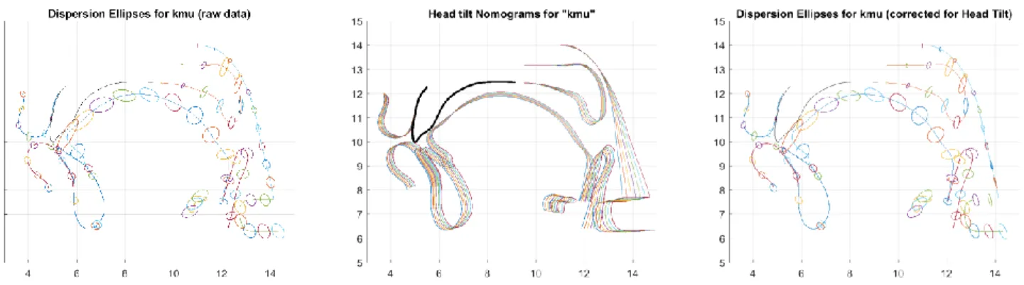
3.5 Head tilt correction
The automatic procedure mentioned above aligns images on the reference image so as to make sure that the skull structures coincide, but it cannot fully control for the change of head tilt, i.e. the angle between the skull and a p parallel to the spine or posterior wall of the pharynx. As we found, the head tilt had a fairly large influence on the shape of all articulators. We have therefore implemented a head tilt correction procedure, based on linear articulatory modelling, considering the head tilt movement as an articulatory component (cf. section 3.7 for a
4 Note that what we call here ‘laryngeal articulator’ for convenience corresponds to the contours of the variable
region of contact of the rear structures of the larynx in the midsagittal plane, namely the transverse and oblique arytenoid muscles and the aryepiglottic folds. During phonation, the laryngeal constrictor mechanism may tighten these muscles slightly, reinforcing the lateral cricoarytenoid contraction necessary to bring the vocal folds into line (Esling et al., 2019). Concomitantly, the visible contact region in the midsagittal plane increases with increasing constriction, whereas it may be considerably reduced during breathing. The horizontal movements of the anterior edge of this region are thus related to vocal fold adduction and to constriction, while its vertical movements are related to vertical movements of the larynx (usually upwards with constriction and downwards during breathing or breathiness). Tracking this contour can thus provide information about laryngeal position and vocal fold state.
13
definition of articulatory models), though not directly related to speech. The head tilt PhTilt was estimated as the z-scored horizontal coordinate of the intersection of the pharyngeal wall measured along a fixed horizontal line just above the larynx region. The contribution of this articulatory variable to the (x / y) coordinates of all articulators was then modelled by a linear regression on PhTilt. Figure 2 displays the nomogram of this component, i.e. the changes in contours when PhTilt varies from -3 to +3): we can observe that the influence of PhTilt decreases from the back to the front of the vocal tract. The head tilt correction then consisted in removing this contribution from the original data. Appendix B illustrates the effects of this head tilt correction for some extreme cases. Further analysis or modelling of the whole set of contours was finally performed on the resulting residues. Note that we checked that all the analyses were actually not much influenced by this correction.
Note also that sometimes the speaker's head was not fully aligned with the mid-sagittal plane – due to subsequent motion of the speaker, which produced parallax errors that could not be compensated for, and which resulted in slight deformations visible in the front region (nose, lips and incisors).
Figure 2. Illustration of the head tilt correction. Left: dispersion ellipses of raw contours plotted for every 15th point;
middle: nomogram of the effect of the head tilt variation; right: dispersion ellipses of the corrected contours (speaker KMU).
3.6 Analysis methods
This section presents the various analytical and modelling methods developed and used in this study, namely display of dispersion ellipses, superposition of individual or mean contours, and articulatory modelling.
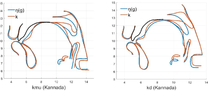
3.6.1 Superposition of contours
The simplest – though very useful – approach to comparing articulations and characterising coarticulatory effects consists in superposing various contours on the top of each other. Though this approach is speaker dependent, since normalising articulatory contours across different speakers is difficult (e.g. Serrurier et al., 2019), the superposition of individual or mean contours for each speaker is very meaningful, as exemplified in Figure 3. Note that the alignment of the images insures that the articulator shapes can be directly compared to each other for a
14
given speaker. For example, we can see in the Figure 3 that velars /k/ and /ŋ(ɡ)/ are produced with roughly the same lingual gesture – a tongue dorsum closure at the boundary between the hard and soft palates (but extending slightly further back for /k/). The positions of the jaw and the lips are relatively similar too. The differences, on the other hand, are in the position of velum/uvula (high for /k/ and low for /ŋ(ɡ)/), as well as the hyoid bone, and, less consistently, the epiglottis and the glottis.
Figure 3. Sample midsagittal mean contours superposition (speaker KD). 3.6.2 Dispersion ellipses
One aim of the work being to characterise the robustness to vocalic coarticulation and compare this robustness between consonants, it was interesting to go one step further from the simple comparison of contours by superposition, and to find ways to estimate the variance of the contours. One classical approach to determine this variance for the tongue is Smoothing Spline ANOVA(SS-ANOVA) (e.g. Davidson, 2006 or Mielke, 2015): this method, applied to contours extracted from ultrasound images, aims to determine confidence interval around the average of contours over several repetitions of the same articulation, and then to compare the different articulations. In practice, the number of repetitions for each item largely amounts to a dozen [8 for Davidson, and apparently more than 20 for Mielke, counting from his Fig. 2], and the variance of the repetitions of the same articulations is low. Besides, the method is useful for contours without large bends – which is the case for contours extracted from ultrasound images where the tip and the root of the tongue are not well visible and thus not taken into account. In its version working with Cartesian X/Y coordinates of the contours (Davidson, 2006), SS-ANOVA works only if Y = f(X) is an injective function of X, i.e. each Y has no more than one corresponding X. As this is not the case of all regions of the tongue due to the large curvature of the vocal tract, Mielke (2015) developed an SS-ANOVA method based on polar coordinates. It is indeed more suitable, but still cannot properly work for
15
retroflex articulations. The extensive contours that we have obtained from our MRI data have complex shapes that cannot be dealt with using SS-ANOVA; moreover, since we aim to study vowel coarticulation, the variance of the repetition of the consonants for the five vowels is large; finally, we have unfortunately only five items for each consonant, which is not suitable for proper statistical analysis.
As we were not able to use SS-ANOVA for our contours, we resorted to a less sophisticated approach to present vocalic coarticulation effects on a consonant in a comprehensive way, as proposed in Badin et al. (2019): we display the mean of the articulations of the same consonant over all vocalic contexts of interest, with a representation of the associated dispersion of contour points, by means of dispersion ellipses drawn at 2 standard deviations around the mean points. This display is illustrated in Figure 4 where we can observe that the tongue tip for /n̪/ has a low variance, whereas the tongue blade region is much more variable.
Appendix C provides the dispersion ellipses for all consonants for both speakers, which can serve as reference.
Figure 4. Example of dispersion ellipses around the points of the mean contour for /n̪/ (speaker KD). Left: only one point every 15th is selected in order to better illustrate the method; right: all points are selected, which allows to see the outlines
of the 2 standard deviations region.
3.7 Articulatory modelling
3.7.1 Principles of articulatory modelling
Due to their complexity, the articulatory contours are difficult to characterise in a meaningful and relevant manner for speech. Articulatory modelling obviously constitutes a way to deal with this issue, as it offers the possibility to boil down the apparent articulatory complexity to a few basic components. As reviewed in Serrurier et al. (2019), linear articulation models based on principal component analysis (PCA) have been successfully used for long to extract and characterise the basic articulatory components of a speaker (e.g. Lindblom et al., 1971 or Serrurier et al., 2008). Such an approach allows to exploit correlations between different shapes of speech organs observed in the tasks in order to determine the independent degrees of freedom (DoF) of the articulators. These DoF correspond to the simple gestures that are linearly uncorrelated and can be performed independently of each other by the
16
articulators (cf. Beautemps et al., 2001). In this study, we used guided PCA which aims to take into account the sole correlations related to biomechanisms while excluding correlations clearly related to pure control strategies (Beautemps et al., 2001). Note that Silva et al. (2016) proposed the “use of objective measures to compare the configurations assumed by the vocal tract during the production of different sounds”; for each speaker, they measured distances in the midsagittal plane at a number of specific locations and normalised them by the maximal distance for each speaker. While this approach might be suitable for normalization purposes, it tends to miss the proper semantics of articulatory parameters.
For each speaker, we have built articulatory models of all segmented organs following the approach described by Badin et al. (2002) or Serrurier et al. (2019). The jaw control parameters, JH (jaw height) and JA (jaw advance), are the z-scored values of the vertical and horizontal coordinates of the lower incisors. Parameter JH is also used as the first control parameter of the tongue. Its main effect is a tongue rotation around a point in the back of the tongue (see Figure 5). The next two parameters, tongue body TB, and tongue dorsum TD, are extracted by PCA from the tongue contour coordinates, excluding the tongue tip region, from which the JH contribution has been removed. They control respectively the front/high vs. back/low and flattening vs. arching/bunching movements of the tongue (see Figure 5). The last two parameters, tongue tip fronting TTF, and tongue tip height TTH, are extracted by PCA from the tongue contour coordinates from which the TB and TD contributions have been removed (see Figure 5). For the upper and lower lips, the z-scored values of the protrusion (ULP, LLP) and height (ULH, LLH) measurements have been used as control parameters in complement to the JH component. This approach leads to somehow lower performances than using the first two PCA components of the JH residue (cf. section 3.7.2 and Table 2), but ensures a better interpretation of these components in terms of phonetics. The models of the other organs (velum, pharynx, hyoid, epiglottis and laryngeal articulator) are simply controlled by their first two PCA components.
To illustrate the general behaviour of these models, we generated articulatory nomograms, i.e. displays of the articulator shapes across the range of control parameters of the model. Figure 5 displays nomograms associated with the components of the various articulators. As we can see in the first two images, the TD parameter controls the arching movement of the posterior region of the tongue towards the velum, accompanied by some lowering of the tongue blade. The second two images show that the TTF parameter is responsible for the lowering of the middle region of the tongue and the fronting of its back region, which seems to be crucial for the raising and retraction of the tongue tip during retroflexion.
18
Figure 5. Nomograms of all articulators for both speakers (left KMU, right KD). Articulatory nomograms of jaw, tongue, lips and velum are displayed as the variations of their shapes for control parameters varying from -3 to +3 by 0.5 steps. Mean contours are drawn in black lines, contours for negative parameter values in green, and those for positive values in
red. Every 10th point is displayed with dots to illustrate the movements of the models points.
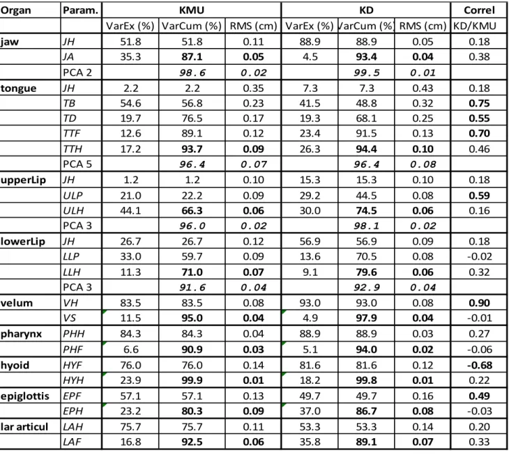
3.7.2 Assessment of the articulatory models
The models have been evaluated in terms of cumulative relative variance explained (VarCum) and of Root Mean Square contour reconstruction Error (RMSE). Table 2 displays the results of the evaluation. These results are consistent with previous similar models elaborated on another speaker (Badin et al., 2006). Overall, the model reconstruction is accurate, with an explained variance between 66 and 98 % (99.8% for the hyoid), and an RMSE between 0.02 and 0.10 cm. Table 2 displays also the performances of the raw PCA models with the same number of parameters as in the guided models for each organ: we observe that the guided models are suboptimal, with a loss of performance with respect to the PCA models between 2.0 and 29.7 %, and 0.02 to 0.04 cm RMSE. The lower performance for the lips may be ascribed to the slight lack of accuracy in the position of the submentale marker (see 3.7.2.1).
19
In order to assess the similarity of articulatory strategies, the Pearson correlation coefficient between the two speakers was estimated for all parameters. Values in Table 2 show that the tongue strategy is rather similar (0.75 for TB, 0.55 for TD, up to 0.70 for TTF, though the jaw is not as much correlated; see the column “Correl.”). Other important similarities are found for the velum (0.90 for VH) or for the upper lip (0.59 for ULP). These similarities are confirmed by the nomograms in Figure 5.
3.7.2.1 Analysis of robustness to extremities errors for the articulatory models
For three specific organs, i.e. the tongue and both lips, the resampling process may introduce errors due to the uncertainty of the localisation of extremities by means of the anatomical landmarks (N2, LL, TT). In order to assess this problem, we have simulated pointing errors for these points and determined the consequences. The projections of the three points N2, LL and TT on the manually edited contours, which are used as anchor points for the resampling of the contours, have been shifted along the contours by an amount randomly chosen in a given range (from 0.1 to 0.5 cm) for the whole corpus. In addition to the original contour data (i.e. no shift), we have obtained another five data sets with increasing error ranges. We have then applied the standard guided PCA modelling approach to each of the six sets articulations, for speaker KD.
We have then made various comparisons of the models obtained from the five datasets with the original one: (cumulated) relative variance explained by each component (VarExCum), RMS reconstruction errors, informal observations of the nomograms, correlations between the articulatory parameters for the different sets.
We observed a very negligible influence of the random shifts of TT on the tongue models and performances. Oppositely, a larger influence of extremities was observed for the lip models. The model on the original data reaches a variance explanation of 94.0% and 92.4% respectively for the upper and lower lips with RMS of 0.026 and 0.038 cm respectively.
Another interesting comparison is the correlation, over the whole corpus, of the articulatory parameters. We have observed that for the lips models a general decrease of the correlations when the extremities shift range increases. The correlations are higher than 0.94 for the 0.1cm range, and higher than 0.66 for the 0.2cm range. We note that for higher ranges some of the correlations are swapped: ULP for the 0.2cm range is correlated with ULH at 0.94, or LLH is correlated with LLP at -0.96. This reflects the fact that the variance of the data, which has been increased by the random shifts, is distributed differently between the first two PCA components.
This was also reflected in the nomograms. A careful inspection of these figures revealed the approximate continuity of semantics (protrusion or height movements) of the components for the different datasets with little dispersion of the markers, and some swaps between some of the components. In conclusion, there are no problems for the tongue, while lips models start to be less reliable for shift ranges greater than 0.3cm, which are not likely to be produced by the expert.
20
Table 2. Performances of the articulatory models by organ parameter (Param.) and speaker (VarEx = relative variance explained by the component; VarCum = cumulative explained variance); figures for the total number of parameters used in the models for each organ are marked in bold. The correlations between KMU and KD parameters are given in the last column; correlations above 0.50 are indicated in bold. In the extra lines for articulators processed with the guided PCA, the performance of the raw PCA model with the same number of parameters is given in non-italics.
Organ Param. Correl
VarEx (%) VarCum (%) RMS (cm) VarEx (%) VarCum (%) RMS (cm) KD/KMU
jaw JH 51.8 51.8 0.11 88.9 88.9 0.05 0.18 JA 35.3 87.1 0.05 4.5 93.4 0.04 0.38 PCA 2 98.6 0.02 99.5 0.01 tongue JH 2.2 2.2 0.35 7.3 7.3 0.43 0.18 TB 54.6 56.8 0.23 41.5 48.8 0.32 0.75 TD 19.7 76.5 0.17 19.3 68.1 0.25 0.55 TTF 12.6 89.1 0.12 23.4 91.5 0.13 0.70 TTH 17.2 93.7 0.09 26.3 94.4 0.10 0.46 PCA 5 96.4 0.07 96.4 0.08 upperLip JH 1.2 1.2 0.10 15.3 15.3 0.10 0.18 ULP 21.0 22.2 0.09 29.2 44.5 0.08 0.59 ULH 44.1 66.3 0.06 30.0 74.5 0.06 0.16 PCA 3 96.0 0.02 98.1 0.02 lowerLip JH 26.7 26.7 0.12 56.9 56.9 0.09 0.18 LLP 33.0 59.7 0.09 13.6 70.5 0.08 -0.02 LLH 11.3 71.0 0.07 9.1 79.6 0.06 0.32 PCA 3 91.6 0.04 92.9 0.04 velum VH 83.5 83.5 0.08 93.0 93.0 0.08 0.90 VS 11.5 95.0 0.04 4.9 97.9 0.04 -0.01 pharynx PHH 84.3 84.3 0.04 88.9 88.9 0.03 0.27 PHF 6.6 90.9 0.03 5.1 94.0 0.02 -0.06 hyoid HYF 76.0 76.0 0.14 81.6 81.6 0.12 -0.68 HYH 23.9 99.9 0.01 18.2 99.8 0.01 0.22 epiglottis EPF 57.1 57.1 0.13 49.7 49.7 0.16 0.49 EPH 23.2 80.3 0.09 37.0 86.7 0.08 -0.03
lar articul LAH 75.7 75.7 0.11 53.3 53.3 0.14 0.20
LAF 16.8 92.5 0.06 35.8 89.1 0.07 0.33
KD KMU
3.7.3 Radar display of articulatory parameters
We have seen that the articulatory parameterization allows to characterise each articulation with a small number of articulatory parameters. Ideally, we would have applied ANOVA to these articulatory parameters to assess the differences between consonants. Unfortunately, each consonant is available in only five vowel contexts, which prevents a pertinent use of ANOVA. Therefore, inspired by Silva et al. (2014), we use a spider or radar chart to
21
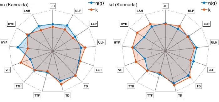
display the main articulatory parameter values simultaneously in a compact way: the superposition of two or three sets of such displays allows a comparison of articulations in terms of main articulatory components, as illustrated in Figure 6. In such plots, values for each component are the means over five vowel contexts; along each radius, the values increase from the minimum on the inner polygon (corresponding to the green contours on the nomograms, Figure 5) to zero on the intermediate polygon, to the maximum on the outer polygon (corresponding to the red contours in the nomograms). For instance Figure 6 shows that the differences between /ŋ(ɡ)/ and /k/ for KMU are mainly related to the velum height (VH, /k/ > /ŋ(ɡ)/), hyoid bone fronting (HYF, /ŋ(ɡ)/ > /k/), and to a lesser degree to other components, including the laryngeal articulator height (LAH), jaw height (JH), upper lip protrusion (ULP, /ŋ(ɡ)/ > /k/), upper lip height (ULH, /k/ > /ŋ(ɡ)/), and the tongue dorsum (TD, /k/ > /ŋ(ɡ)/). For KD, the main differences are in the velum height, the hyoid bone height (HYH), and to a lesser degree in the upper lip protrusion (all /k/ > /ŋ(ɡ)/).
Figure 6. Example of radar charts (KMU left, KD right).
4 Results
The presentation of results is organised by place differences (Section 4.1), manner differences (Section 4.2), and patterns of coarticulation (Section 4.3). Within the first two sections, the results are further sub-divided by types of contrast – by manner, place, or both.
22
4.1 Place differences within manner classes
4.1.1 Place contrasts in stops/affricates
4.1.1.1 Contrasts among coronals
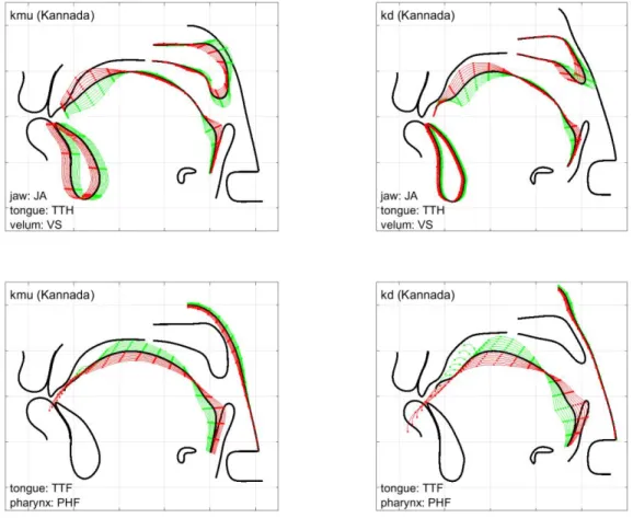
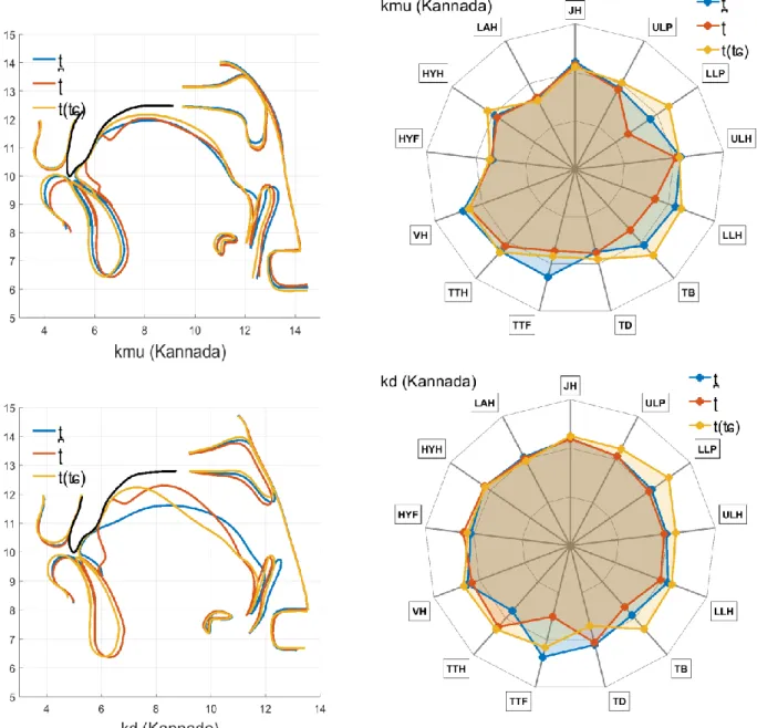
The results for coronal stops/affricates are presented in Figure 7, separately by speaker. Overlaid average articulator contours are displayed on the left, while radar displays are presented on the right. In each case, we begin by providing general descriptions of three articulations represented in overlaid contours, and follow by a review of differences in articulatory parameters based on radar displays. In articulatory descriptions, we are using the delineation of upper and lower articulator areas from Catford (1988).
For KMU, we can see that /t̪/ can be described as an apico-laminal denti-alveolar/post-alveolar stop, as the constriction is produced by both the tip and the blade, and extends over a large area from the upper teeth to the post-alveolar region. The consonant is produced with an overall convex tongue, a somewhat raised tongue body, and a slightly more retracted lower posterior part of the dorsum. The second consonant, /ʈ/, is an apical/sublaminal post-alveolar stop, as it is apparently produced with both the tip and the underside in the postalveolar area. Its tongue shows a small concavity between the blade and the tongue body; the tongue body and the tongue dorsum are convex, and overall similar to /t̪/. Among other characteristics of this consonant are the considerably lowered/retracted jaw, a lowered/less protruded lower lip, and a small sublingual cavity. The third consonant, the affricate /t(tɕ)/ is produced as an apico-laminal denti-alveolar/post-alveolar stop, with the constriction being similar to /t̪/, but extending slightly further back. Its tongue is convex and considerably raised (palatalised) compared to the other stops; the posterior portion of the tongue (its tongue dorsum) is similar to that of /ʈ/ (and more fronted than for /t̪/, while the root is fronted compared to the other two consonants. In addition, the affricate is produced with a lowered larynx, and both lips being considerably protruded. The somewhat higher/more front position of the hyoid bone appears to reflect the raising of the tongue body. Turning to articulatory parameters illustrated in the radar plot, differences among the three consonants are mainly related to the components TTF (the tongue tip is the most front for /t̪/, compared to /ʈ/ and /t(ʨ)/), TB (the tongue body is the highest for /t(ʨ)/ and the lowest for /ʈ/), and LLP and LLH (the lower lip is most protruded and highest for /t(ʨ)/ and least protruded and lowest for /ʈ/).
For KD, /t̪/ can also be classified as an apico-laminal denti-alveolar stop; it has a relatively flat/weakly convex tongue shape, a raised/retracted dorsum, and a slightly retracted root. /ʈ/ is an apical/sublaminal post-alveolar/prepalatal stop (thus showing a contact somewhat further than for KMU), with a concavity between the blade and the tongue body, and a convex tongue body/middle, and a somewhat flattened/fronted tongue dorsum. It also shows a slightly lower/retracted jaw, a sublingual cavity, and a weaker velopharyngeal port closure, compared to the other consonants. /t(tɕ)/ is an apico-laminal denti-alveolar/post-alveolar stop, which is strongly palatalised (showing a considerably raised and fronted, strongly convex tongue body). The tongue middle and the dorsum for this consonant are flattened, while the jaw is fronted and the lips are protruded. The tongue-palate
23
contact for /t(ʨ)/ is quite extensive. Considering articulatory parameters in the radar plot, differences are mainly related to TTF (the tongue tip is most retracted for /ʈ/), TTH (the tongue tip is the lowest for /t̪/), TB (the tongue body is the highest for /t(ʨ)/), TD (the tongue dorsum is the least arched for /t(ʨ)/), and LLP (the lower lip is most protruded for /t(ʨ)/).
Figure 7. Overlaid average contours (left) and radar displays of articulatory parameters (right) for stops/affricate at the dental /t̪/ vs. retroflex /ʈ/ vs. alveolopalatal /t(ʨ)/ places for both speakers (top KMU, bottom KD).
24
Overall, both speakers consistently distinguish the dental vs. retroflex contrast by the fronting/backing movement of the tongue tip and the raising/lowering movement of the tongue body, while differing in their use of additional components to implement this contrast.
Note that some between-speaker differences in the components used to implement the dental vs. retroflex contrast can be attributed to somewhat different articulatory targets for both sounds. As seen in Figure 7 (left column), the /t̪/ constriction is more posterior for KMU (the tongue blade contact extending from the upper teeth to the alveolar ridge) than for KD (primarily the tip touching the upper teeth). For /ʈ/, the patterns are reversed: the constriction is more anterior for KMU (the tip touching the alveolar/post-alveolar region) than for KD (the tip or the under-side contact extending further into the post-alveolar region). Somewhat unexpectedly, one of the tokens of /ʈ/ (/iʈi/) was produced by KD with a lower velum (as would be expected for /ɳ/): this is possibly a strategy for maintaining the voicing – that is a secondary cue to retroflexion in Kannada – during the sustained consonant. Interestingly, similar nasalization of the retroflex /ʈ/ was observed in a separate MRI dataset from two Malayalam speakers.
It is also worth noting that neither speaker produces /ʈ/ with a noticeable backing of the tongue dorsum or tongue root, relative to /t̪/, as might be expected of retroflexes (see Section 1). In fact, the opposite is observed for KD. This is consistent with observations made by Kochetov et al. (2014) based on ultrasound data. The considerably higher tongue body and – for KD – the more front tongue dorsum/root than for /t̪/ is consistent with ultrasound results reported by Kochetov et al. (2016). Importantly, however, the MRI data further show that these contrasts are not limited to differences in tongue posture, but involve other parameters, such as small-scale adjustments of the lips and the velum.
4.1.1.2 Other contrasts
While our focus here is on coronal contrasts, it is worth considering articulatory parameters distinguishing coronals from non-coronals. Among other place contrasts in stops, both speakers differentiated the bilabial /p/ from the lingual /t̪/ primarily by ULH (a lower position of the upper lip). They differentiated /k/ from /t̪/ by TD (a higher tongue dorsum for the velar) and TTF (a more retracted tongue tip for the velar). It should be also noted that the velar stop was produced by both speakers with a fairly front constriction – in the posterior palatal, rather than the velar region. KD in particular, produced /k/ with the fronting of the entire tongue and the epiglottis, as well as some raising of the hyoid bone and the laryngeal articulator. Additional figures can be found in Appendix D.
4.1.2 Place contrasts in nasals
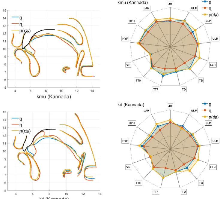
4.1.2.1 Contrasts among coronals
The results for coronal nasals – dental, retroflex, and alveolopalatal (phonetic) – are presented in Figure 8. For KMU, /n̪/ can be described as an apico-laminal denti-alveolar nasal, produced with a weakly convex tongue body, and convex tongue dorsum. /ɳ/ is an apical/sublaminal post-alveolar (and possibly prepalatal) nasal, with
25
a concavity between the blade and the tongue body, a convex front portion of the tongue body, and a flattened tongue dorsum. It also shows somewhat less protruded lips and a sublingual cavity. /ɲ(ʥ)/ is an apico-laminal denti-alveolar nasal, which is weakly palatalised (showing a convex and slightly raised tongue body). The tongue dorsum is convex as well, while being very similar in shape to /n̪/; the jaw is somewhat raised/fronted, while the lips are more protruded. All three nasals, as expected, show a widely open velopharyngeal port. In the radar plot, we can see that the differences among three nasals are mainly related to TTF (the tongue tip is most posterior for /ɳ/, compared to /n̪/ and /ɲ(ʥ)/), TB (the tongue body is the least front/high for /ɳ/, at least in its posterior region, however, also related to a concomitant retraction of the tip region, as can be seen in the TB nomogram in Figure 5), and to a lesser degree in TD (the tongue dorsum is somewhat less arched for /ɳ/ at the mid and lower further back) and LLP (the lower lip is most protruded for /ɲ(ʥ)/ and least protruded for /ɳ/).
For KD, /n̪/ is an apico-laminal denti-alveolar nasal, with a relatively small area of contact. The tongue shows a slight concavity between the blade and the tongue body, a moderately convex tongue body and the tongue dorsum. /ɳ/ is a sublaminal prepalatal/palatal nasal (with the contact produced by a strongly curled tongue in a fairly posterior portion of the palate). The tongue-palate contact is extensive. The tongue shows a substantial concavity between the blade and the tongue body, while the tongue body middle is convex and the tongue dorsum is flattened/fronted. Other characteristics of the consonant include a somewhat lowered/backed jaw, a slightly retracted tongue root, a lowered larynx, and a large sublingual cavity. /ɲ(ʥ)/ is an apico-laminal denti-alveolar nasal, which is palatalised (produced with a raised convex tongue body); the tongue dorsum is moderately convex (being similar to /n̪/ and more posterior than for /ɳ/), while the jaw is raised/fronted, and the lower lip slightly protruded. The higher position of the hyoid bone for /ɲ(ʥ)/ seems to reflect the raising/fronting of the tongue body, while the lower position of this organ (as well as the larynx) for /ɳ/ is likely due to the lowering of the tongue dorsum. All three nasals are produced with a widely open velopharyngeal port. As seen in the radar plot, parameter differences among three nasals are mainly related to TTF (the tip is the most posterior for /ɳ/), TB (the tongue body is the most retracted/lowest for /ɳ/ and the most advanced/highest for /ɲ(ʥ)/), and LLH (the lower lip is the higher for /ɲ(ʥ)/). In addition, we can notice a general lowering of the hyoid bone and the laryngeal articulator for the retroflex /ɳ/ (seen on HYH and LAH).
Thus, both speakers make use of TTF and TB to distinguish the dental vs. retroflex contrast in nasals, while showing smaller and less consistent differences between the alveolopalatal and the dental (mainly involving articulators other than the tongue). Note that the retroflex /ɳ/ is produced with a considerable tongue tip curling behind the alveolar ridge (sub-apical postalveolar/palatal), and more so for KD than KMU. Both speakers also show some fronting/lowering of the tongue dorsum for /ɳ/, compared to the other two articulations (and this difference is more extensive than was observed for stops). Unexpectedly, the alveolopalatal nasal is produced by KD with a more extended upper teeth contact than the dental nasal. Note also that the constriction location for the
26
alveolopalatal nasal, as produced by both speakers, is less extensive than we observed for the palatal affricate, and hardly overlaps with that of the retroflex counterpart.
Among other coronal contrasts involving nasals, no difference was observed between /n̪/ and /n̪(d̪)/, nor between /ɳ/ and /ɳ(ɖ)/. The lack of the former difference is in contrast with previous descriptions, which attribute to these consonants distinct places – alveolar and dental respectively (Upadhyaya (1972): /n/ vs. /n̪(d̪)/).
Figure 8. Overlaid average contours (left) and radar displays of articulatory parameters (right) for nasals at the dental /n̪/ vs. retroflex /ɳ/ vs. alveolopalatal /ɲ(ʥ)/ places for both speakers (top KMU, bottom KD).
27
4.1.2.2 Other nasal contrasts
Among place contrasts involving non-coronal stops, /m/ was differentiated from coronal nasals by ULH (a lower position of the upper lip for /m/). /ŋ(ɡ)/ was different from /n̪/ primarily in TD (a higher tongue dorsum), and TTF (a more retracted tongue tip). These differences are fully expected for contrasts between coronals and labials/velars. No difference was observed between /m/ and a nasal in the nasal+stop cluster (/m(b)/). Further additional figures can be found in Appendix D.
4.1.3 Place contrasts in fricatives
4.1.3.1 Contrasts among coronals
The results for coronal fricatives – the phonemically dental, retroflex, and alveolopalatal sibilants – are presented in Figure 9.
For KMU, /s̪/ is a laminal denti-alveolar fricative, with a flattened anterior portion of the tongue body (and a very weak concavity between the blade and the tongue body). The middle of the tongue is fairly convex, while the larynx is lowered. /ʂ/ is a laminal alveolar/post-alveolar fricative, with the entire tongue raised and convex. It also shows a slightly fronted jaw and a raised/protruded lower lip. The constriction and the tongue shape for /ɕ/ are almost identical to /ʂ/, with the differences being in a slightly more protruded tongue tip and more fronted jaw for the former. Both /ʂ/ and /ɕ/ show a relatively extensive constriction area and a small sublingual cavity. In terms of parameters shown in the radar plot, differences between the fricatives are mainly related to TTH (the tip is the lowest for /s̪/ compared to /ʂ/ and /ɕ/) and TTF (the tip is the most advanced for /s̪/). The posterior sibilants /ʂ/ and /ɕ/ show hardly any differences in the tongue parameters, while exhibiting some minor difference in LLH (a somewhat higher lower lip for /ɕ/).
For KD, /s̪/ is an apico-laminal denti-alveolar fricative, with a very flat tongue behind the constriction, a somewhat raised and convex tongue dorsum, a slightly retracted tongue root, and lowered larynx. /ʂ/ is a laminal alveolar/post-alveolar fricative, which is strongly palatalised (with a substantially raised and fronted tongue body, which is strongly convex). The tongue dorsum is flattened, while the tongue root is slightly fronted, and lips are protruded. As for the other speaker, the articulation of /ɕ/ by KD is near-identical to /ʂ/, with the difference being mainly in a slightly more protruded tongue tip and a higher lower lip for the alveolopalatal. Both consonants show relatively extensive constriction areas. Most parameter differences, based on the radar plot, are between /s̪/ on the one hand and /ʂ/ and /ɕ/ on the other. Primarily, these differences are in TTH (the tongue tip is the lowest for /s̪/), TTF (the tongue tip is the most advanced for /s̪/), TB (the tongue body is least front/lower for /s̪/), and TD (the tongue dorsum is most arched for /s̪/). In addition, both lips show the least protrusion for /s̪/ compared to the other two sibilants (LLP and ULP). Differences between /ʂ/ and /ɕ/ are essentially absent, with the exception of the relatively minor ones involving LLH and HYF (the lower lip is slightly higher and the hyoid being more back for /ɕ/ than /ʂ/).