Large-scale confinement and small-scale clustering of floating particles in stratified turbulence

HAL Id: hal-01386444

https://hal.archives-ouvertes.fr/hal-01386444

HAL is a multi-disciplinary open access archive for the deposit and dissemination of sci-entific research documents, whether they are pub-lished or not. The documents may come from teaching and research institutions in France or

L’archive ouverte pluridisciplinaire HAL, est destinée au dépôt et à la diffusion de documents scientifiques de niveau recherche, publiés ou non, émanant des établissements d’enseignement et de recherche français ou étrangers, des laboratoires

Large-scale confinement and small-scale clustering of

floating particles in stratified turbulence

Alessandro Sozza, Filippo de Lillo, Stefano Musacchio, G Boffetta

To cite this version:

Alessandro Sozza, Filippo de Lillo, Stefano Musacchio, G Boffetta. Large-scale confinement and small-scale clustering of floating particles in stratified turbulence. Physical Review Fluids, American Physical Society, 2016, 1 (5), pp.052401(R). �10.1103/PhysRevFluids.1.052401�. �hal-01386444�

Large-scale confinement and small-scale clustering of floating

particles in stratified turbulence

A. Sozza1

, F. De Lillo1

, S. Musacchio2

and G. Boffetta1 1

Department of Physics and INFN, Universit`a di Torino, via P. Giuria 1, 10125 Torino, Italy

2

Universit´e de Nice Sophia Antipolis, CNRS, LJAD, UMR 7351, 06100 Nice, France

(Dated: October 24, 2016)

Abstract

We derive a simple model, valid within the Boussinesq approximation, for the dynamics of small buoyant particles in stratified turbulence, in presence of a mean linear density profile. By means of extensive direct numerical simulations, we investigate the statistical distribution of particles as a function of the two dimensionless parameters of the problem. We find that vertical confinement of particles is mainly ruled by the degree of stratification, with a weak dependency on the particle properties. On the contrary, small scale fractal clustering is found to depends on the particles relaxation time and is only slightly dependent on the flow stratification. The implications of our findings for the formation of thin phytoplankton layers are discussed.

Particles of density different from that of the surrounding fluid do not follow the motion of fluid particles, and generate inhomogeneous distributions even in incompressible flows [1]. This phenomenon is crucial in a variety of instances, from cloud formation in the atmosphere, to the dynamics of plankton in the ocean and lakes, to industrial applications [2–4]. The formation of inhomogeneous distributions in turbulent flows is also interesting from a theoretical point of view and, in recent years, analytical, numerical and experimental studies led to significant advances in the understanding of this process [5–10]. Most of the studies have considered the case of inertial particles which accumulate in regions of high vorticity (light particles) or high strain (heavy particles) [5, 7, 11], as a consequence of the accelerations induced by the flow. Recent works have studied the interaction between gravity and turbulent accelerations in the dynamics of heavy particles. In particular, it has been shown that turbulence can increase their settling velocity with respect to still fluid, by pushing particles in regions of downward flow [12, 13]. In presence of density fluctuations, gravity also affects the flow itself as in the case of stratified turbulence, which finds many applications in natural flows [14, 15], e.g. ocean dynamics in the presence of the pycnocline resulting from temperature and salinity variations [16, 17]. Little is known about the distribution of floating particles in stratified turbulence, in spite of its relevance for applications. Recent works have studied the effect of stratification on the clustering of heavy [18] and light [19] particles, the formation of tangling clustering in stratified turbulence [20, 21] and the effect of a vertical confinement in homogeneous turbulence [22].

One of the most remarkable examples of confinement of particles in the ocean is the for-mation of the so-called thin phytoplankton layers (TPL): aggregations of phytoplankton and zooplankton at high concentration with thickness from centimeters to few meters, extending up to several kilometers horizontally and with timescale from hours to days [23]. Among the possible mechanisms of formation of TPLs, convergence to a depth of neutral buoyancy has been proposed for non-swimming species and aggregates, such as diatoms and marine snow, which are often observed to accumulate in presence of strong stratification [24].

In this work we investigate, by means of direct numerical simulations (DNS), the distri-bution of small buoyant particles transported in a turbulent stratified flow in the regime in which gravity dominates over the fluid acceleration. In this regime we consider a simple model for the particle motion which neglects inertial acceleration and balance the Stokes drag with the buoyancy forces. We study both the large scale vertical distribution and the

small scale clustering of particles as a function of the relevant parameters. We find that small scale (fractal) clustering is determined by the particles relaxation time with a weak dependency on the degree of stratification. Conversely, the vertical confinement of particles is found to be mostly controlled by stratification. When rescaled to the typical parameters in the ocean, our results predict a fractal distribution for particles of few millimeter size.

FIG. 1. (Color online). Isopycnal surfaces θ = z corresponding to the density ρ0 for a run at F r = 0.2. The points represent the (fractal) distribution of bouyant particles with τ = 0.1 in the stationary state.

We consider a fluid linearly (and stably) stratified in the direction z of gravity g = (0, 0, −g) with a constant mean density gradient dρ/dz = −γ. Within the Boussinesq approximation, the motion for the incompressible velocity field u(x, t) is ruled by

∂u ∂t + u · ∇u = − 1 ρ0 ∇p + ν∇2 u− N2 θˆz + f (1) ∂θ ∂t + u · ∇θ = u · ˆz + κ∇ 2 θ (2)

together with ∇ · u = 0. The scalar field θ(x, t), which in the above equations has the dimension of a length, represents the deviations of the local density from the linear vertical profile, ρ = ρ0 − γ(z − θ). ν is the kinematic viscosity, κ the density diffusivity and N =

(γg/ρ0) 1_/2

to sustain turbulence. In the inviscid, unforced limit (ν = κ = f = 0) equations (1-2) conserve the total energy, sum of kinetic and potential contributions, E = 1

2h|u| 2 i +1 2N 2 hθ2 i where h...i denotes the average over the domain.

The velocity v of a small inertial particle transported by the flow u generated by (1) evolves according to [27] dv dt = β du dt − v− u τp + (1 − β)g (3)

where β = 3ρ/(ρ + 2ρp) is the density ratio (ρp is the density of the particle of radius a) and

τp = a 2

/(3νβ) is the viscous (Stokes) time. By introducing the covelocity w = v − u [7] we can rewrite (3) as dw dt = −(1 − β) du dt − w τp + (1 − β)g . (4) Without loss of generality, we fix the particle density ρp = ρ0 and, consistently with the

Boussinesq approximation in (1-2), we neglect the first term in the r.h.s of (4) (as (1 − β) ≃ (ρ0− ρ)/ρ0 is a small parameter). Moreover, having in mind the dynamics of plankton in

the ocean, we have that typical turbulent accelerations are much smaller than g. We remark that additional terms (e.g. the Basset history term) are in general present in (3) but they would give a negligible contribution within the above approximation [25]. Considering now the limit of small particles we obtain at the first order in τp an explicit expression for the

velocity of the floater v whose position x evolves according to dx

dt = v = u − 1

τ(z − θ)ˆz (5)

where we have used the fact that (1 − β)g ≃ 2 3N

2

(z − θ) and we have introduced the particle relaxation time τ ≡ 3/(2N2

τp) to the isopycnal surface of density ρ0. This surface, defined

implicitly by the relation z = θ(x, y, z), will be denoted as h(x, y), keeping in mind that in general it can be multivalued. The model (5) which, to our knowledge has never been studied before, represents the simplest model for the dynamics of floaters in stratified flows and physically represents the balance between the Stokes drag and the buoyancy forces. A similar model has been developed and studied in [21]. Its validity is based on the assumptions of small density fluctuations (i.e. validity of the Boussinesq approximation) and small Stokes time of the particle. More general models, starting from the complete equation (3) can be considered, at the price of increased complexity and number of parameters [19].

Although the fluid velocity u is incompressible, the velocity field transporting the floaters is not since ∇ · v = −(1 − ∂θ/∂z)/τ which is in general nonzero. This expression represents

the rate of contraction of the phase space (here the configuration space) under the dynamics. When it is negative we expect that trajectories of floaters will collapse on a (dynamical) fractal attractor in the phase space. Examples of the attractor are displayed in Fig. 1 which shows that the large scale confinement in the vertical direction coexists with a small scale clustering with fractal distribution on the isopycnal surface.

-L/2

0

L/2

0

L/2

L

-L/2

0

L/2

0

L/2

L

-L/2

0

L/2

0

L/2

L

-L/2

0

L/2

0

L/2

L

FIG. 2. (Color online). Vertical (x, z) sections of isopycnal surfaces h (black points) for F r = 0.3 (upper row) and F r = 1.0 (lower row) together with the positions of bouyant particles (green points) with relaxation numbers R = 1.0 (left column) and R = 60.0 (right column).

We have integrated the Boussinesq equations (1-2) in a cubic domain of size L = 2π with periodic boundary conditions by means of a fully parallel pseudo-spectral code at resolution up to M = 256. Turbulence is generated by a δ-correlated in time, isotropic forcing f which is active on a spherical shell of wavenumber around kf = 2π/Lf and which

pumps energy at the fixed rate ε. These parameters define, together with the Brunt-V¨ais¨al¨a frequency, the Froude number F r ≡ ε1_/3

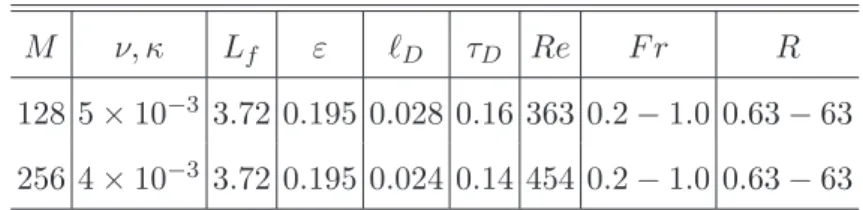
M ν, κ Lf ε ℓD τD Re F r R 128 5 × 10−3 3.72 0.195 0.028 0.16 363 0.2 − 1.0 0.63 − 63 256 4 × 10−3 3.72 0.195 0.024 0.14 454 0.2 − 1.0 0.63 − 63

TABLE I. Parameters of the simulations. N resolution, ν and κ kinematic viscosity and diffusivity, Lf = 2π/kf forcing scale, ε energy input rate, ℓD = (ν3/ε)1/4 Kolmogorov scale, τD = (ν/ε)1/2 Kolmogorov timescale, Re = L4_f/3ε1_/3

/ν, F r = ε1_/3

k_f2/3/N and R = τ /τD. The actual range of R depends on the value of F r. All the simulations are performed at Schmidt number Sc = ν/κ = 1.

Another relevant parameter in stratified turbulence is the buoyancy Reynolds number Reb =

ε/(νN2

) defined in terms of the ratio of the buoyancy (Ozmidov) scale ℓB = ε 1_/2

/N3_/2

to the dissipative scale ℓD = ν3/4/ε1/4 as Reb = (ℓB/ℓD)4/3, in analogy to the usual Reynolds

number Re = (Lf/ℓD)4/3. These three numbers are not independent since Reb ∝ F r2Re and

Reb = 1 discriminates between stratified-viscous flow (Reb < 1) and stratified turbulence

(Reb > 1) [28]. Our simulations are mostly within the turbulent regime, with Reb in the

range 2 ≤ Reb ≤ 72. We remark that in stratified turbulence the energy dissipation rate

is in general different from the injection rate ε as a fraction of the input is converted into potential energy [26]. In our simulations this difference is small and therefore, following the literature [28], we use the injection rate to define small scale quantities.

Together with (1-2), we integrated equation (5) for the particle motion for a set of 10 classes of floaters characterized by different values of τ in the range 0.1 ≤ τ ≤ 10.0. In presenting the results, this time will be made dimensionless with the Kolmogorov time τD = (ν/ε)

1_/2

by introducing the relaxation number R ≡ τ /τD. We remark that R is

proportional to the inverse of the usual Stokes number St ≡ τp/τD which is based on

the particles Stokes time τp [7]. Table I reports the most important parameters of the

simulations.

In Figure 2 we show vertical sections (at y = 0) of the isopycnal surface h (obtained from the solution of z = θ(x, y, z)) together with positions of the particles on the same sections, for different values of the parameters F r and τ . It is evident that the isopycnal surface h is almost flat for strong stratification and it becomes more bent (and multivalued) as F r increases. Figure 2 shows also the effect of the relaxation time τ on the particles. When R = τ /τD < 1 the floaters are practically attached to the isopycnal surface, while their

positions depart from the surface h by increasing τ .

0.2

0.4

0.6

0.8

1

1.2

1.4

0.2

0.3

0.4

0.5

0.6

0.7

0.8

0.9

1

σ

Fr

R=1.3

R=3.1

R=6.3

R=31

R=63

FIG. 3. (Color online). Standard deviations σz of the PDFs of particle vertical position as a function of F r for different values of R at Re = 363. The solid black line represents the standard deviation σh of the isopycnal surface. Inset: slope γ of the standard deviations obtained from the fit σz = σ0+ γF r as a function of R.

The distribution of the vertical displacement z of particles with respect to their equi-librium position in the absence of turbulence, z = 0, is found to be Gaussian in the wide range of parameters investigated. The standard deviations σz of these vertical distributions

of particles for different values of F r and R are shown in Fig. 3. We obtain a linear scaling of σz on F r, with a coefficient γ which shows a (weak) dependency on R. For stronger

stratification, F r ≤ 0.3, the standard deviation is almost independent on R and the slope converge to γ ≃ 0.84, a feature which can be understood by looking at the plots in Fig. 2. The effect of the relaxation term in (5) is to allow the particle to detach from the level z = θ and to remain “suspended” for a time of order τ before feeling the vertical velocity towards

the isopycnal surface. Because in stratified turbulence vertical velocity is suppressed [28], there is no mechanism which ejects particles far from the surface. Therefore, as shown by Fig. 2, the vertical region visited by particles (measured by σz) reflects the vertical extension

of the isopycnal surface (given by its standard deviation σh) which, by definition, is

inde-pendent on τ . The linear dependence of σh on F r shown in Fig. 3 can be understood within

the framework of stratified turbulence, as a manifestation of the presence of the so-called vertical shear layers [29] and the associated vertical correlation scale of velocity Lv.

Phys-ically this scale represents the vertical displacement for converting injected kinetic energy into potential energy and can be estimated dimensionally as Lv ≃ U/N (U is a typical large

scale velocity) and therefore one obtains Lv ∝ F r, i.e. the linear scaling shown in Fig. 3.

10

10

10

10

10

10

-10

-5

0

5

10

p(

ζ

)

σ

ζ

/

σ

FIG. 4. (Color online). Probability density functions of the variable ζ = z −θ computed on particle positions for Re = 454, F r = 1.0 and R = 1.4 (red line with square), R = 7.0 (blue line with circle) and R = 70 (pink line with triangle). The black line is a Gaussian.

of the variable ζ = z − θ computed along particle trajectories. The dynamics of ζ is given by the time evolution of the field θ along the trajectory of a floater and gives (neglecting the diffusive term) d(z − θ)/dt = −(z − θ)(1 − ∂θ/∂z)/τ . In the absence of fluctuations (θ = 0) this equation would simply represent the linear relaxation of particles towards the isopycnal layer z = 0 [22]. This is not achieved since the term ∂θ/∂z is fluctuating without a definite sign. Figure 4 shows the normalized PDF of the variable ζ for three different values of τ at F r = 1.0. It is evident that the statistics is neither Gaussian nor scale invariant and the PDF develops large tails for small relaxation times [31]. These large fluctuations are due to the folding of the isopycnal surface. In correspondence of a fold the stratification is inverted, (1 − ∂θ/∂z) changes sign and (z − θ) grows exponentially (assuming that the field θ is quenched) until the particle reaches the nearest branch, above or below, of the isopycnal. This mechanism, which is enhanced at large F r, produces large fluctuations of the distance between the particles and the isopycnal surface, and causes the development of large tails in the PDF of ζ.

As already discussed, floating particles moving according to (5) are transported by a compressible velocity field and are therefore expected to relax on a (dynamical) fractal subset of the physical space, as shown in the examples of Fig. 1. In order to characterize this subset, and its dependence on the parameters, we have measured the correlation dimension D2 of particle distribution, defined as the scaling exponent of the probability of finding two

particles at distance less than r: P (|x1− x2| < r) ∝ rD2 as r → 0 [30]. The maximum value

D2 = 3 denotes uniformly distributed particles, while D2 < 3 indicates fractal patchiness

with smaller D2 corresponding to more clustered distributions and increased probability of

finding pairs of particles at close separation. Figure 5 shows D2 as a function of R for

different values of F r. As the model (5) has been derived under the assumption of small τp/τD, its validity is guaranteed above a minimum R which depends on F r. In Fig. 5 we

plot the values of D2 corresponding the parameter space which satisfies the above condition.

In the limit R ≫ 1, for which v → u in (5), floaters move as fluid particles in an incom-pressible velocity and therefore remain uniformly distributed in the volume with D2 = 3.

We remark that this limit is equivalent to taking τp → 0 in the general model of inertial

particles (3). For smaller values of R the fractal dimension decreases and reaches a value D2 ∼ 1 for the stronger stratifications and the smallest relaxation time. This value

1

1.5

2

2.5

3

1

10

D

R

Fr=0.2

Fr=0.3

Fr=0.4

Fr=0.6

Fr=1.0

FIG. 5. (Color online). Correlation dimension D2 versus relaxation time R for different values of stratification parameter F r. The error bars represent the fluctuation of the local scaling exponent in the fitting range of scales (0.1η ≤ r ≤ 10η). Inset: the correlation dimension D2 plotted as a function of F r for different values of R.

in Fig. 1).

The dependence of the fractal dimension on the degree of stratification is shown in the inset of Fig. 5. We observe that, in general, D2 is virtually independent on F r for F r ≥ 0.5.

This is in contrast with the (large scale) vertical confinement shown in Fig. 4 which displays a strong (linear) dependence on F r and a weak dependence on St.

In order to test the applicability of our results to the formation of TPLs we provide a simple example using the typical values observed for diatom-dominated marine snow [24]. Let us assume an energy dissipation rate ε ≃ 10−8 m2s−3 (τ

D ≃ 10 s) and a Brunt-V¨ais¨al¨a

frequency N ≃ 0.1 s−1. The Froude number corresponding to N ≃ 0.1 s−1 in our simulations

the size of the particles (see Fig. 3). Conversely, the distribution of the particles within the layer can be very different. Aggregates of size a ≃ 0.5 cm have a relaxation time τ ≃ 18 s which corresponds to R = 1.8, at which we observe clustering at small scales with D2 < 2 (Fig. 5). Smaller aggregates or single cells of size a = 0.1 cm correspond to

R ≃ 45 and, according to our results, would distribute almost homogeneously (with a fractal dimension close to 3) within the thin layer. Our model allows estimating the characteristic time for the formation of TPLs. In particular, in the case of strong stratification in which the isopycnals are almost flat, our model predicts that the floaters converge exponentially toward the isopycnal ρ = ρp, with a relaxation time τ = 3/(2N2τp). Further field and

laboratory experiments could provide evidence of this stratification-induced patchiness in thin phytoplankton layers.

Beside the applications to thin layers, our results are of general interest as they describe quantitatively and for the first time how the combination of turbulence and stratification generates both large scale confinement and small scale fractal patchiness in a suspension of buoyant particles.

ACKNOWLEDGMENTS

This article is based upon work from COST Action MP1305, supported by COST (Eu-ropean Cooperation in Science and Technology).

[1] M.W. Reeks, Flow Turbulence Combust. 92, 3 (2014).

[2] W.W. Grabowski, and L.P. Wang, Growth of cloud droplets in a turbulent environment, Annu. Rev. Fluid Mech. 45, 293 (2013).

[3] S. Post, J. Abraham, Modeling the outcome of dropdrop collisions in Diesel sprays, J. Multi-phase Flow 28, 997 (2002).

[4] J. Seinfeld, Atmospheric Chemistry and Physics of Air Pollution, J. Wiley and Sons (1986). [5] K.D. Squires and J.K. Eaton, Preferential concentration of particles by turbulence, Phys.

Fluids A 3, 1169 (1991).

turbulent flows, Phys. Rev. Lett. 86, 2790 (2001).

[7] J. Bec, Fractal clustering of inertial particles in random flows, Phys. Fluids 15, L81 (2003). [8] G. Boffetta, F. De Lillo and A. Gamba, Phys. Fluids 16, L20 (2004).

[9] J. Bec, L. Biferale, M. Cencini, A. Lanotte, S. Musacchio, and F. Toschi, Heavy particle concentration in turbulence at dissipative and inertial scales, Phys. Rev. Lett. 98, 084502 (2007).

[10] I. Fouxon, Distribution of Particles and Bubbles in Turbulence at a Small Stokes Number, Phys. Rev. Lett. 108, 134502 (2012).

[11] L.P. Wang and M.R. Maxey, Settling velocity and concentration distribution of heavy particles in homogeneous isotropic turbulence, J. Fluid Mech. 256, 27 (1993).

[12] J. Bec, H. Homann and S.S. Ray, Gravity-driven enhancement of heavy particle clustering in turbulent flow, Phys. Rev. Lett. 112, 184501 (2014).

[13] K. Gustavsson, S. Vajedi and B. Mehlig, Clustering of particles falling in a turbulent flow, Phys. Rev. Lett. 112, 214501 (2014).

[14] D. Lilly, Stratified Turbulence and the Mesoscale Variability of the Atmosphere, J. Atmos. Sci. 40, 749 (1983).

[15] J. Riley and M. Lelong, Fluid motions in the presence of strong stable stratification, Annu. Rev. Fluid Mech. 32, 613 (2000).

[16] S.A. Thorpe, “An Introduction to Ocean Turbulence”, Cambridge Univ. Press (2007). [17] R.G. Williams and M.J. Follows, “Ocean Dynamics and the Carbon Cycle”, Cambr. Univ.

Press (2011).

[18] M. van Aartrijk and H.J.H. Clercx, Preferential concentration of heavy particles in stably stratified turbulence, Phys. Rev. Lett. 100, 254501 (2008).

[19] M. van Aartrijk and H.J.H. Clercx, Vertical dispersion of light inertial particles in stably stratified turbulence: The influence of the Basset force, Phys. Fluids 22, 013301 (2010). [20] A. Eidelman, T. Elperin, N. Kleeorin, B. Melnik and I. Rogachevskii, Tangling clustering of

inertial particles in stably stratified turbulence, Phys. Rev. E 81 056313 (2010).

[21] T. Elperin, N. Kleeorin, M. Liberman and I. Rogachevskii, Tangling clustering instability for small particles in temperature stratified turbulence, Phys. Fluids 25 085104 (2013).

[22] M. De Pietro, et al, Clustering of vertically constrained passive particles in homogeneous isotropic turbulence, Phys. Rev. E 91, 053002 (2015).

[23] W.M. Durham and R. Stocker, Thin phytoplankton layers: characteristics, mechanisms, and consequences, Annu. Rev. Marine Sci. 4, 177 (2012).

[24] A.L. Alldredge, et al, Occurrence and mechanisms of formation of a dramatic thin layer of marine snow in a shallow Pacific fjord , Mar. Ecol. Prog. Ser. 233, 1 (2002).

[25] S. Olivieri, F. Picano, G. Sardina, D. Iudicone and L. Brandt, The effect of the Basset history force on particle clustering in homogeneous and isotropic turbulence, Phys. Fluids 26 041704 (2014).

[26] A. Sozza, G. Boffetta, P. Muratore-Ginanneschi and S. Musacchio, Dimensional transition of energy cascades in stably stratified forced thin fluid layers, Phys. Fluids 27, 035112 (2015). [27] M.R. Maxey and J.J. Riley, Equation of motion for a small rigid sphere in a nonuniform flow,

Phys. Fluids 26, 883 (1983).

[28] G. Brethouwer, P. Billant, E. Lindborg, J.M. Chomaz, Scaling analysis and simulation of strongly stratified turbulent flows, J. Fluid Mech. 585, 343 (2007).

[29] P. Billant, J.M. Chomaz, Self-similarity of strongly stratified inviscid flows, Phys. Fluids 13, 1645 (2001).

[30] G. Paladin and A. Vulpiani, Anomalous scaling laws in multifractal objects, Phys. Rep. 156, 147 (1987).

[31] D.A. Birch, W.R. Young, P.J.S. Franks, Plankton layer profiles as determined by shearing, sinking, and swimming, Limnol. Oceanogr. 54, 397 (2009).