Multi-Class Leveraged $k$-NN for Image Classification

HAL Id: hal-00664606

https://hal.inria.fr/hal-00664606

Submitted on 31 Jan 2012

HAL is a multi-disciplinary open access

archive for the deposit and dissemination of

sci-entific research documents, whether they are

pub-lished or not. The documents may come from

teaching and research institutions in France or

abroad, or from public or private research centers.

L’archive ouverte pluridisciplinaire HAL, est

destinée au dépôt et à la diffusion de documents

scientifiques de niveau recherche, publiés ou non,

émanant des établissements d’enseignement et de

recherche français ou étrangers, des laboratoires

publics ou privés.

Paolo Piro, Richard Nock, Frank Nielsen, Michel Barlaud

To cite this version:

Paolo Piro, Richard Nock, Frank Nielsen, Michel Barlaud. Multi-Class Leveraged k-NN for Image

Classification. Proceedings of the 10th Asian Conference on Computer Vision, ACCV 2010, November

8-12, 2010, Queenstown, New Zealand, 2010, Queenstown, New Zealand. �hal-00664606�

Multi-Class Leveraged k-NN

for Image Classification

Paolo Piro1_{, Richard Nock}2_{, Frank Nielsen}3_{, and Michel Barlaud}1

1 _{University of Nice-Sophia Antipolis / CNRS, France} 2 _{CEREGMIA, University of Antilles-Guyane, France}

3 _{Sony CSL / LIX, Ecole Polytechnique, France}

Abstract. The k-nearest neighbors (k-NN) classification rule is still an essential tool for computer vision applications, such as scene recognition. However, k-NN still features some major drawbacks, which mainly reside in the uniform voting among the nearest prototypes in the feature space.

In this paper, we propose a new method that is able to learn the “relevance” of

prototypes, thus classifying test data using a weighted k-NN rule. In particular,

our algorithm, called Multi-class Leveraged k-nearest neighbor (MLNN), learns the prototype weights in a boosting framework, by minimizing a surrogate expo-nential risk over training data. We propose two main contributions for improving computational speed and accuracy. On the one hand, we implement learning in an inherently multiclass way, thus providing significant computation time reduc-tion over one-versus-all approaches. Furthermore, the leveraging weights enable effective data selection, thus reducing the cost of k-NN search at classification time. On the other hand, we propose a kernel generalization of our approach to take into account real-valued similarities between data in the feature space, thus enabling more accurate estimation of the local class density.

We tested MLNN on three datasets of natural images. Results show that MLNN significantly outperforms classic k-NN and weighted k-NN voting. Furthermore, using an adaptive Gaussian kernel provides significant performance improve-ment. Finally, the best results are obtained when using MLNN with an appro-priate learned metric distance.

1 Introduction

In this paper, we address the task of image categorization. This task aims at automati-cally classifying images into a predefined set of scene categories, like the natural scenes represented in Fig.1. (See Sec.3.1for a detailed description of the databases we used in our experiments). Despite lots of works, much remains to be done to challenge hu-man level perforhu-mances, not only because there is a huge number of natural categories that should be considered in general. In fact, images carry only parts of the informa-tion that is used by humans to categorize, and parts of the informainforma-tion available from images may be highly misleading: for example, natural image categories may exhibit high intra-class variability (i.e., visually different images may belong to the same cat-egory) and low inter-class variability (i.e., distinct categories may contain images that are visually similar).

highway tall building open country mountain

inside city street coast forest

Fig. 1. The first dataset we used in our experiments consists of 8 categories of natural scenes [1]. k-nn DatasetBoosting Dataset Query 1 Query n (PS) k-nn SVM SVM Query n Query 1 k-nn Classes 1 Classes n Classes 1 Classes n k-nn

Fig. 2. Optimizing k-NN via MLNN (up, blue) and SVM-KNN [2] (down, green). MLNN uses a boosting algorithm before being presented any query, while SVM-KNN learns support vectors after each query is presented. Bold rectangles indicate induction steps (PS = prototype selection; see text for details).

For the purpose of automatic classification of images, the k-NN classification has shown to be very effective [3]. Its use is supported by a wide spectrum of arguments, ranging from the field of philosophy to that of mathematics [2]. The simplicity of the method — use the labeled neighbor(s) of a query to predict its class — makes it a good candidate for further improvements, desirable in part because of statistical and compu-tational drawbacks [2]. So far, the literature has favoured two main ways to cope with these issues: improve classification accuracy by means of local classifiers [2,4,5,6], or filter out ill-defined examples [7], with intermediate approaches [8]. Many of these algo-rithms can be viewed as primers to improve the (continuous) estimation of class mem-bership probabilities [9], but none has completely succeeded in this task. This problem has been reformulated by Marin et al. [10] as a strong advocacy for the formal trans-position of boosting to k-NN classification. This issue is challenging as k-NN rules are indeed not induced, whereas formal boosting algorithms combine two induction steps,

inducing so-called strong classifiers by combining weak classifiers (also induced). Pre-viously, Athitsos and Sclaroff [11] had already proposed an approach to bring the boost-ing principle into the k-NN classification framework. However, their method consisted in “boosting” the distance measure, i.e., learning a combination of metric distances that could improve the generalization of classifier. Furthermore, their classification frame-work was not intrinsically multiclass, as they formulated the problem as binary learning on random triplets of training data.

In this paper, we tackle the issue of integrating k-NN in a boosting framework from a different perspective. In particular, our algorithm, called MLNN, induces a multiclass leveraged k-nearest neighbor rule that generalizes the uniform k-NN rule, using the ex-amples directly as weak hypotheses (that we also call prototypes). Our MLNN method does not need to learn a distance function, as it directly operates on the top of k-nearest neighbors search. Furthermore, it does not require an explicit computation of the feature space, thus preserving one of the main advantages of prototype-based methods. Com-pared to the well-known SVM-k-NN local learning approach [2], MLNN also speeds up query processing: instead of learning a local classifier for each query, MLNN per-forms learning upwards, once and for all, and does not need to be run again or updated depending on queries (Fig.2). Finally, the most significant advantage of MLNN lies in its ability to find out the most relevant prototypes for categorization, allowing to filter out the remaining less reliable examples. Experimentally, significant data reductions are observed with a simultaneous increase in categorization performances.

In Sec.2we present our MLNN approach, along with the statement of its theoretical properties. In order not to laden the paper’s body, the proofsketches of the results have been postponed to an appendix. Then, Sec.3displays the behavior of MLNN on three standard databases of real-world image categorization. Finally, we conclude with some observations (Sec.4).

2 Method

2.1 Problem statement and notations

In this paper, we address the task of multiclass image categorization. It consists in as-signing an image to one of several predefined categories (or classes, or labels). Instead of splitting the multiclass problem in as many one-versus-all (binary) classification problems — a frequent approach in boosting [12] — we directly tackle the multiclass problem, following Zou et al [13]. For a given query image, we compute its

classifica-tion score for all categories. While we basically use this vector for single-label

predic-tion using the category with the maximum score, our algorithm can be straightforwardly extended to multilabel prediction and ranking [12]. We suppose given a set S of m an-notated images. Each image is a training example (x, y), where x is the image feature vector and y the class vector that specifies the category membership of the image. In particular, the sign of component ycgives the positive/negative membership of the

ex-ample to class c (c = 1, 2, ..., C). Inspired by the multiclass boosting analysis of Zou et al [13], we constrain the class vector to be symmetric, i.e.:!C

c=1yc = 0, by setting: yc˜= 1, yc!=˜c=−_C−11 , where ˜c is the true image category. Furthermore, we denote by K(xi, xj)a symmetric similarity kernel on the pair of examples xi, xj.

2.2 (Leveraged) k-Nearest Neighbors

The vanilla k-NN rule is based on majority vote among the k-nearest neighbors in set S, to predict the class of query xq. It can be defined as the following multiclass classifier h =_{hc, c = 1, 2, ..., C}: hc(xq) = 1 k " i∼kq [yic> 0] , (1)

where hc ∈ [0, 1] is the classification score for class c, i ∼k qdenotes an example

(xi, yi) belonging to the k-nearest neighbors of xq and square brackets denote the

indicator function.

In this paper, we propose to generalize (1) to the following leveraged k-NN rule

h!₌ {h! c}: h!c(xq) = T " j=1 αjK(xq, xj)yjc∈ R , (2) where prediction h!

ctakes values in all R. In (2), we have introduced the three following

elements to generalize (1):

– leveraging coefficients αj, that provide a weighted voting rule instead of uniform

voting;

– kernel K, which takes into account “soft” (real-valued) similarities between query

xq and prototypes xj, instead of “hard” selection of the most similar (k-NN)

pro-totypes;

– size T of the set of prototypes that are allowed to vote.

This last point is particularly interesting for computational purposes, as our classifica-tion rule actually involves only a (possibly sparse) subset of the training data as pro-totypes to be used at query time. Indeed, a prototype selection step is to be performed while training our classifier, in order to determine the most relevant subset of training data, i.e., the so-called prototypes, forming a set P ⊆ S (Figure2). The prototypes are selected during the training phase, which consists in fitting their coefficients αj, while

removing the least relevant annotated data from S. 2.3 Multiclass surrogate risk minimization

In order to fit our leveraged classification rule (2) onto training set S, we focus on the minimization of a multiclass surrogate4_{(exponential) risk:}

εexp#_h!_, S$=. 1 m m " i=1 exp%_−ρ(h!_{, i)}& _{, (3)} 4_{We call surrogate a function that upperbounds the risk functional we should minimize, and}

where: ρ(h!, i) = 1 C C " c=1 yich!c(xi) (4)

is the multiclass edge of classifier h!_{on training example x}

i. In particular, this edge

averages over the C classes the “goodness of fit” of classifier h!_{on example (x} i, yi),

thus being positive iff the prediction agrees with the example’s annotation. Therefore, counting the number of negative edges enables to quantify the so-called empirical risk,

i.e., the actual misclassification rate on the training data, as follows: ε0/1#_h!_, S$=. 1 m m " i=1 ' ρ(h!_{, i) < 0}( _{. (5)}

Rather than directly tackling the problem of minimizing ε0/1 _{— which is not}

differ-entiable and often computationally hard to minimize [14] — we concentrate on the optimization of surrogate (3), which is an upper bound of the empirical risk.

In order to solve this optimization, we propose a boosting-like procedure, i.e., an iterative strategy where the classification rule is updated by adding a new prototype (xj, yj)(weak classifier) at each step t (t = 1, 2, . . . , T ), thus updating the strong

classifier (2) as follows:

h(t)

c (xi) = h(tc−1)(xi) + δjK(xi, xj)yjc. (6)

(j is the index of the prototype chosen at iteration t.) Using (6) into (4), and then plug-ging it into (3), turns the problem of minimizing (3) to that finding δjwith the following

objective: arg min δj m " i=1 wi· exp {−δjrij} . (7)

In (7), we have defined wi as the weighting factor, depending on the past weak

classi-fiers: wi= exp ) −_C1 C " c=1 yich(tc−1)(xi) * , (8)

and rij as a pairwise term only depending on training data:

rij= K(xi, xj) 1 C C " c=1 yicyjc. (9)

Finally, taking the derivative of (7), the global minimization of surrogate risk (3) amounts to fitting δjso as to solve the following equation:

m

"

i=1

Algorithm 1: MULTI-CLASSLEVERAGEDk-NN MLNN(S)

Input: S = {(xi, yi) , i = 1, 2, ..., m , yi∈ {− 1

C−1, 1}

C }

Let rij=. _C1 !Cc=1K(xi, xj)yicyjc (11)

Let αj← 0, ∀j = 1, 2, ..., m

Let wi← 1/m, ∀i = 1, 2, ..., m

for t = 1, 2, ..., T do

[I.0] Weak index chooser oracle: Let j ← WIC(_{{1, 2, ..., m}, t);} [I.1] Compute δjsolution of:

m " i=1 wirijexp{−δjrij} = 0 ; (12) [I.2] Let wi_{← w}iexp(−δjrij), ∀i : j ∼ki ; (13) [I.3] Let αj← αj+ δj Output: h! c(xq) =!_j∼kq αjcyjc, ∀c = 1, 2, . . . , C

2.4 MLNN: Multi-Class Leveraged k-NN rule

Pseudocode of MLNN is shown in Alg. 1. The main ingredient to compute leveraging coefficients relies on the so-called edge matrixRwith general entry ri,j(Eq.9). This

term depends on the pairwise similarity between two training examples, as it is given by the kernel, as well as on the ground-truth annotations. Indeed, it combines a “labeling” term, which determines the sign, i.e., being positive iff labels of i and j agree, with a “geometric” term, which influences the magnitude, i.e., being larger when the two examples are closer to each other in the feature space.

We distinguish the following two cases, depending on which kernel is selected:

k-NN kernel In the most basic setting, i.e., when using k-NN kernel, term K(xi, yi)

behaves like an indicator function that only selects the k-NN of i. Therefore, in this case (9) simplifies to:

rij . = + ₁ C !C c=1yicyjc if j ∼ki 0 otherwise (14)

and (10) has the following closed-form solution:

δj ← (C_{− 1)}2 C log , (C− 1)w+ j wj− -, (15) with: w_j+= " i: rij>0 wi, w−j = " i: rij<0 wi. (16)

general kernel When using any kernel, entries of the edge matrix (Eq.9) are real-valued and, in general, not sparse. Moreover, the equation (10) is transcendental, thus not admitting a closed-form solution. Hence, we compute the solution numer-ically, implementing a Newton’s iterative method. This method gives the following approximation at step k + 1, given the previous one at step k:

δ(k+1)= δk+ !m i=1wirijexp{−δ(k)rij} !m i=1wir2ijexp{−δ(k)rij} . (17)

A critical setting for obtaining quick convergence of the solution is the initializa-tion. Here, we propose to initialize the algorithm with the root of a linearized ver-sion of Eq. (10): δ(0)= !m i=1wirij !m i=1wir2ij . (18)

A suitable choice for the kernel is the Radial Basis Function (RBF), which provides “smooth” pairwise similarities between feature points:

K(xi, xj) = exp + −||xi− xj|| 2 2σ2 . , (19)

where parameter σ may be either constant or adapted to the local sample density (e.g., one may set σ = ρk(xi), where ρk(xi)is the k-NN distance to xi, thus

“enlarging” the window size where training data are sparser.) In particular, in the following experiments we use a Gaussian kernel that is truncated to the first k near-est neighbors, thus providing a straightforward generalization of the k-NN kernel. In this case the edge matrix writes as follows:

rij=. ) 1 C !C c=1exp / −||xi−xj2σ2 ||2 0 yicyjc if j ∼k i 0 otherwise . (20)

Another ingredient of MLNN is more common to boosting algorithms: MLNN operates on a set of weights wi (i = 1, 2, ..., m) defined over training data. These

weights are repeatedly updated, such that those of mislabelled examples are increased, and vice-versa.

At each iteration t of the algorithm, a weak index chooser oracle WIC(_{{1, 2, ..., m}, t)} determines index j ∈ {1, 2, ..., m} of the example to leverage (step I.0). Various choices are possible for this oracle. The simplest is perhaps to compute Eq. (16,12) for all the training examples. δj in Eq. (12) can indeed be used to obtain a local measure of the

class density [14], which is as better as δj gets large. This simple oracle thus picks j

maximizing δj:

j← WIC({1, 2, ..., m}, t) : δj = max j∈{1,2,...,m}δ

t

j . (21)

This oracle allows an example to be chosen more than once, thus letting its leveraging coefficient αjbe updated several times (step I.3). It is known that, in order to be

Cast in the setting of MLNN, this constraint precisely supports prototype selection, as

T is an upperbound for the number of examples with non-zero leveraging coefficients. MLNN shares the property with boosting algorithms of being resources-friendly: since computing the leveraging coefficients scales linearly with the number of neigh-bors, the time complexity bottleneck of MLNN does not rely on boosting, but rather on the complexity of k-NN search. Furthermore, notice that, when whichever w+

j or w−j is

zero, δjin (12) is not finite. There is a simple way to eliminate this drawback, inspired

by [12]: we add 1/m to both the numerator and the denominator of the fraction in the log term of (12). This smoothes out δj, guaranteeing its finiteness without impairing

convergence of MLNN.

In the following section, we provide formal details about the boosting analysis of MLNN.

2.5 Properties of MLNN

Two fundamental theorems hold for MLNN.

Theorem 1 MLNN converges with T to h!_{realizing theglobal minimum of the} expo-nential risk (3).

MLNN is a specialization of a very general learning algorithm which keeps the same convergence guarantee when replacing the surrogate risk (3) by elements of a broad class of surrogates risk [15,14].

The second theorem provides a convergence rate for MLNN, which is based on a fundamental assumption on weak classifiers.

Theorem 2 Let pj .

= w_j+/(w+_j + w_j−). If the following weak index assumption (WIA)

holds for τ ≤ T steps in MLNN:

(WIA) There exist some γ > 0 and η > 0 such that the following two inequalities hold

for index j returned by WIC({1, 2, ..., m}, t):

|pj−1/C| ≥ γ , (22)

(w+_j + w_j−)/_||w||1≥ η . (23)

Then: ε0/1_(h!_{,S) ≤ exp(−} C

C−1ηγ2τ ).

(Proofsketch in appendix) Ineq. (22) is the usual weak learning assumption, used to analyze classical boosting algorithms [16,12], when considering examples as weak classifiers. A weak coverage assumption (23) is needed as well, because insufficient

coverage of the reciprocal neighbors could easily wipe out the surrogate risk reduction

due to a large γ in (22). In the framework of k-NN classification, choosing k not too small is enough for theWIA to be met for a large number of boosting rounds τ, thus determining a potential harsh decrease of εexp_(h!_,

S). This is important, as a big

dif-ference with classical boosting algorithms (e.g. AdaBoost [16]) is that oracle WIC(., .) has only access to m different weak classifiers, i.e., one per example. Finally, the bound in Theorem2shows that classification (22) may be more important than coverage (23) for nearest neighbors.

3 Experiments

In this section, we present experimental results of MLNN with different kernel set-tings and comparison with both k-NN and ITML [6], which is a state-of-the-art metric learning algorithm. In particular, our experiments aim at evaluating the effect of UNN sparse prototype selection on the classification accuracy. For this purpose, we measured the classification performances when varying the number of prototypes retained at test time. In MLNN, prototype selection is carried out by setting T < m, which corre-sponds to retaining at most T relevant prototypes. When running the other methods, we carried out random prototype selection and averaged the results over a number of iterations.

3.1 Scene categorization

We validated our MLNN algorithm on three well-known image categorization databases. 8-cat: firstly proposed by [1], includes 2,688 color images grouped into eight

cate-gories: 360 coast, 328 forest, 374 mountain, 410 open country, 260 highway, 308 inside of cities, 356 tall buildings, and 292 street (Fig.1).

13-cat: adds five more categories of gray-scale images to the 8-cat database [17]: 241 suburb residence, 174 bedroom, 151 kitchen, 289 living room, and 216 office. 15-cat: includes 13-cat database plus two more categories (gray-scale images) [18]:

315 store, and 311 industrial.

In the following section we report results obtained by splitting each database in two distinct subsets, one for training, the other for test. We always used about 2,000 randomly selected training images. Namely, 250 images per category were selected from the 8-cat database, 150 from the other two datasets. The remaining images were used for testing. In our experiments, we mostly concentrated on evaluating the trade-off between classification accuracy and computational time, as provided by selecting a sparse prototype dataset from the training data. In particular, fixing the number of prototypes amounts to fixing the computational cost of classification, as this latter only depends on the cost of k-NN search on the prototype set. (So as for k-NN, a random sample of the training set was selected and results were averaged over a number of random sampling realizations.) All the results we present were obtained with k = 11 and pre-processing Gist features [1] with PCA down to dimension d = 128.

We compared different implementations of our MLNN algorithm. In particular, we tested:

– MLNN with the basic setting, i.e., the uniform k-NN kernel of Eq. (14); – WMLNN, i.e., MLNN with fixed-size Gaussian kernel (19) (with σ = 0.25); – AdaWMLNN, i.e., MLNN with adaptive-size Gaussian kernel (_√ 19) (with σ =

2ρk(xi), ρk(xi)being the k-NN distance from example xi);

– MLNN “one-versus-all”, i.e. Alg. 1 with C = 2 applied to each category indepen-dently (considering examples in the current category as “positives”, the remaining ones as “negatives”).

Furthermore, we compared our method with different k-NN–based classification methods, which either rely on metric learning or not. Namely, we tested:

– classic non-parametric k-NN voting;

– weighted k-NN (Wk-NN) voting with Gaussian weights, as proposed by Philbin et al. [19]; we used (19) with σ = 1 as a weighting factor;

– k-NN voting combined with ITML metric learning [6].

We tested all these methods for a fixed number of prototypes, i.e., for a fixed compu-tational cost of classification. In particular, a random sample of the training set was selected and results were averaged over a number of random sampling realizations.

Finally, we integrated the ITML method with MLNN in order to provide a unique method for addressing simultaneously both the choice of the metric distance and the rejection of “noisy” examples, which are the two fundamental issues of k-NN classifi-cation.

3.2 Categorization results

The categorization test consists in assigning each test image to one of the predefined categories. We measured the overall performance rate as the mean Average Precision (mAP), which is the average of the classification rates for each category.

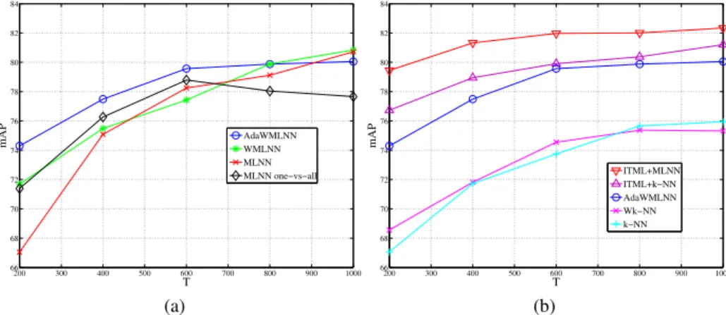
In Fig.3(a)we compare the results of MLNN with the abovementioned settings. In-terestingly, these results show the significant improvement provided by using a “smooth” kernel for learning the prototypes. Namely, the adaptive-size kernel provides the best performances. Furthermore, the gap over the basic MLNN is more consistent when re-taining less prototypes, as AdaMLNN enables a finer class density estimation even with very sparse examples (see, for instance, the performance gap of 7% between MLNN and AdaWMLNN for T = 200). Furthermore, notice that the multiclass version of our algorithm outperforms the one-versus-all implementation (gap between 1% and 3%). Hence, our multiclass MLNN not only is much less computationally expensive than one-versus-all MLNN, as it avoids to run the boosting procedure C times indepen-dently, but also provides better classification accuracy.

On the same 8-cat database we compared AdaWMLNN to k-NN voting with or without metric learning (Fig.3(b)). First of all, we notice that our AdaWMLNN method significantly outperforms k-NN and Wk-NN, i.e., non-learned voting rules (up to 6% improvement). Then, performances of our method are overall comparable to those of ITML, being slightly inferior to them, but the computational cost of MLNN is con-siderably lower than that of metric learning. Finally, our results show that, when com-bined with a metric learning strategy, MLNN is able to significantly outperform all the other classification methods, thus enabling a significant accuracy improvement over the state-of-the-art (up to 3% when retaining few prototypes, see for example performance at T = 200).

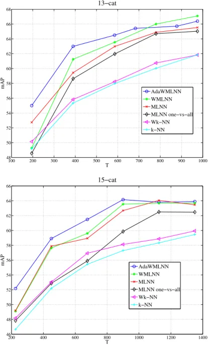
In Fig.4we focus on a more extensive comparison between regular MLNN and classic k-NN on the 13-cat and 15-cat datasets. Here, we report the mean Average Precision as a function of the number of prototypes per category. (Since this number varies from category to category, we report the average number of prototypes over all

200 300 400 500 600 700 800 900 1000 66 68 70 72 74 76 78 80 82 84 T mAP AdaWMLNN WMLNN MLNN MLNN one−vs−all (a) 200 300 400 500 600 700 800 900 1000 66 68 70 72 74 76 78 80 82 84 T mAP ITML+MLNN ITML+k−NN AdaWMLNN Wk−NN k−NN (b)

Fig. 3. Experimental results of categorization on 8-cat database in terms of mAP as a function of the number of prototypes, for k = 11 and Gist descriptors of dimension

d = 128(after PCA). (a) Comparison between 3 different implementations of MLNN

and one-versus-all MLNN. (b) Comparison between MLNN with adaptive Gaussian kernel (AdaWMLNN), k-NN, weighted k-NN and MLNN one-versus-all (UNN). categories.) Notice that the gap between the two methods is most significant when re-taining less than half prototypes, namely 6% improvement with 80 prototypes on 8-cat database, 7% with only 60 prototypes for both 13-cat and 15-cat. Besides considerably improving precision over k-NN, we also drastically reduce the computational complex-ity of classification, which deals with finding nearest neighbors on a sparse dataset (gain up to a factor 4 when discarding half prototypes).

4 Conclusion

In this paper, we have proposed a novel boosting algorithm, MLNN, which learns a leveraged k-NN rule following the minimization of a multiclass surrogate (exponen-tial) risk. This rule generalizes k-NN to weighted voting. Under mild learning and coverage assumptions, MLNN convergence is proven to be exponentially fast. Exper-iments on benchmark image categorization databases display that MLNN is signifi-cantly more accurate than k-NN (up to 6%), achieving very significant improvement on image databases with only few thousand images. Since the number of weak hy-potheses available for boosting is in the order of the number of images, improvements may rapidly become dramatic as databases get larger. MLNN also provides us with a very simple and efficient prototype selection method reducing the cost of searching for neighbors at classification time. MLNN precision is comparable with that of a state-of-the-art metric learning method [6]. Since MLNN is still fully compatible with any underlying distortion and data structure for k-NN search, it also take advantage from learning a metric distance, thus simultaneously solving both major issues of k-NN vot-ing: selection of a suitable metric distance and rejection of “noisy” prototypes. Last but

100 200 300 400 500 600 700 800 900 1000 48 50 52 54 56 58 60 62 64 66 68 T mAP 13−cat AdaWMLNN WMLNN MLNN MLNN one−vs−all Wk−NN k−NN 200 400 600 800 1000 1200 1400 46 48 50 52 54 56 58 60 62 64 66 T mAP 15−cat AdaWMLNN WMLNN MLNN MLNN one−vs−all Wk−NN k−NN

Fig. 4. Performance of MLNN with different settings (see the paper for details) com-pared to k-NN and weighted k-NN as a function of the number of prototypes per class for 13-cat (4(a)) and 15-cat (4(b)) datasets.

not least, MLNN is simple and modular enough, so that it can be easily extended to work on global image descriptors (like Bags of Features, Fisher Kernels ...)

References

1. Oliva, A., Torralba, A.: Modeling the shape of the scene: A holistic representation of the spatial envelope. Int. J. of Comp. Vision42 (2001) 145–1752,9

2. Zhang, H., Berg, A.C., Maire, M., Malik, J.: Svm-knn: Discriminative nearest neighbor classification for visual category recognition. In: CVPR’06. (2006) 2126–21362,3

3. Boiman, O., Shechtman, E., Irani, M.: In defense of nearest-neighbor based image classifi-cation. In: CVPR’08. (2008) 1–82

4. Hastie, T., Tibshirani, R.: Discriminant adaptive nearest neighbor classification. IEEE Trans. PAMI18 (1996) 607–6162

5. Paredes, R.: Learning weighted metrics to minimize nearest-neighbor classification error. IEEE Trans. PAMI28 (2006) 1100–1110 Member-Vidal, Enrique.2

6. Davis, J.V., Kulis, B., Jain, P., Sra, S., Dhillon, I.S.: Information-theoretic metric learning. In: ICML’07. (2007) 209–2162,9,10,11

7. Brighton, H., Mellish, C.: Advances in instance selection for instance-based learning algo-rithms. Data Mining and Knowledge Disc.6 (2002) 153–1722

8. Zuo, W., Zhang, D., Wang, K.: On kernel difference-weighted k-nearest neighbor classifica-tion. Pattern Anal. Appl.11 (2008) 247–2572

9. Holmes, C.C., Adams, N.M.: Likelihood inference in nearest-neighbour classification mod-els. Biometrika90 (2003) 99–112 2

10. Marin, J.M., Robert, C.P., Titterington, D.M.: A Bayesian reassessment of nearest-neighbor classification. J. of the Am. Stat. Assoc. (2009)2

11. Athitsos, V., Sclaroff, S.: Boosting nearest neighbor classi.ers for multiclass recognition. In: CVPR ’05: Proceedings of the 2005 IEEE Computer Society Conference on Computer Vision and Pattern Recognition (CVPR’05) - Workshops. (2005) 453

12. Schapire, R.E., Singer, Y.: Improved boosting algorithms using confidence-rated predictions. Machine Learning37 (1999) 297–3363,8

13. Zou, H., Zhu, J., Hastie, T.: New multicategory boosting algorithms based on multicategory fisher-consistent losses. Annals of Applied Statistics2(4) (2008) 1290–13063

14. Nock, R., Nielsen, F.: Bregman divergences and surrogates for learning. IEEE Trans. PAMI 31 (2009) 2048–20595,7,8

15. Bartlett, P., Jordan, M., McAuliffe, J.D.: Convexity, classification, and risk bounds. J. of the Am. Stat. Assoc.101 (2006) 138–1567,8

16. Freund, Y., Schapire, R.E.: A Decision-Theoretic generalization of on-line learning and an application to Boosting. Journal of Comp. Syst. Sci.55 (1997) 119–1398

17. Fei-Fei, L., Perona, P.: A bayesian hierarchical model for learning natural scene categories. CVPR (2005) 524–5319

18. Lazebnik, S., Schmid, C., Ponce, J.: Beyond bags of features: Spatial pyramid matching for recognizing natural scene categories. In: CVPR. (2006) 2169–2178 9

19. Philbin, J., Chum, O., Isard, M., Sivic, J., Zisserman, A.: Lost in quantization: Improving particular object retrieval in large scale image databases. In: Proceedings of the IEEE Con-ference on Computer Vision and Pattern Recognition. (2008)10

5 Appendix

Proofsketch of Theorem2 Without loss of generality and to simplify notations, assume that j = t in Alg. 1, and denote wjthe weight vector on which we compute (12) — thus,

the weight update in (13) gives wt+1, and the first weight vector is w1. Let us denote

Zt .

=_||wt+1||1the normalization coefficient for weights, and ˜w(t+1)i .

= wti/Ztthe

normalized weight of example (xi, yi)in the (t + 1)thweight vector. Few derivations

lead: εexp(h!,S) = T 1 t=1 Zt . (24)

We now compute an upperbound for Zt, removing the t index for readability. For this

objective, we extend notations (16) to the normalized tilda notation above, and let )=. mini,t:K(xi,xt)>0K(xi, xt)and )

.

= maxi,tK(xixt). Due to the lack of place, we

make the proof in the simpler case where ) = ) = 1. We obtain:

Z = m " i=1 ˜ wiexp (−δjrij)≤ ˜w+j exp # −#C_C− 1log # (C_{− 1)wj}+ w−_j $$ + +(1_{− ˜}w−_{j − ˜}w+_j) + ˜w−_j exp # # Clog # (C− 1)w+ j w− j $$ = = 1_{− ˜}w−j − ˜w+j + C C_{− 1} % (C_{− 1) ˜}w+j &1 C%_w˜− j &1−1 C ₌ = 1− ( ˜wj−+ ˜w+j)  1 −C % (C_{− 1) ˜˜}w+ j &1 C %_w˜_˜− j &1−1 C C_{− 1}   (25)

where we have used the shorthands ˜˜wj+ .

= wj+/(wj++w−j)and ˜˜w−j .

= w−j/(wj−+w+j).

Using theWIA (23) and the fact that 1 − x ≤ exp(−x), we obtain from (25):

Z_{≤ exp}+_−η%1_{− f( ˜˜}wj+) &, , (26) f (x)=. C C− 1((C− 1)x) 1 C ₍₁− x)1− 1 C _{, x}∈ [0, 1] .

f (x)is concave on [0, 1] and admits a maximum in x = 1/C; Assuming theWIA (22),

we get | ˜˜wj+−1/C| ≥ γ. If x ≤1/C− γ, then f(x) ≤ g−(γ), and if x ≥1/C+ γ, then f (x)≤ g+(γ), with: g₋(γ)= (1. _{− Cγ)}C1 2 1 + C C− 1γ 31−1 C , g+(γ) . = (1 + Cγ)C1 2 1₋ C C− 1γ 31−1 C .

But it can be shown that both g−(γ)and g+(γ)can be upperbounded by g(γ) = 1 −

Cγ2_/(C

− 1), ∀C ≥ 2, ∀γ ∈ [0, 1]. Plugging the bound in (26), we obtain:

Z_{≤ exp}'_−η#1_{− g( ˜˜}w+j) $( = exp 4 −_CC − 1ηγ 2 5 .

Finally, Z ≤ 1 because 0 ≤ fC(x)≤ 1 for any x ∈ [0, 1], and (24) yields εexp(h!,S) ≤

exp(_−Cηγ2_{τ /(C}

− 1)). Using the fact that ε0/1_(h!_,

S) ≤ εexp_(h!_,

S) yields the proof