FGT Poverty Measures and the Mortality Paradox: Theory and Evidence

(1)

HAL Id: halshs-00845490

https://halshs.archives-ouvertes.fr/halshs-00845490

Preprint submitted on 17 Jul 2013

HAL is a multi-disciplinary open access

archive for the deposit and dissemination of

sci-entific research documents, whether they are

pub-lished or not. The documents may come from

teaching and research institutions in France or

L’archive ouverte pluridisciplinaire HAL, est

destinée au dépôt et à la diffusion de documents

scientifiques de niveau recherche, publiés ou non,

émanant des établissements d’enseignement et de

recherche français ou étrangers, des laboratoires

FGT Poverty Measures and the Mortality Paradox:

Theory and Evidence

Mathieu Lefebvre, Pierre Pestieau, Grégory Ponthière

To cite this version:

Mathieu Lefebvre, Pierre Pestieau, Grégory Ponthière. FGT Poverty Measures and the Mortality

Paradox: Theory and Evidence. 2013. �halshs-00845490�

(2)

WORKING PAPER N° 2013 – 23

FGT Poverty Measures and the Mortality Paradox:

Theory and Evidence

Mathieu Lefebvre

Pierre Pestieau

Grégory Ponthière

JEL Codes: I32

Keywords: Income-differentiated mortality, FGT poverty measures

P

ARIS

-

JOURDAN

S

CIENCES

E

CONOMIQUES

48, BD JOURDAN – E.N.S. – 75014 PARIS TÉL. : 33(0) 1 43 13 63 00 – FAX : 33 (0) 1 43 13 63 10

(3)

FGT Poverty Measures and the Mortality

Paradox:

Theory and Evidence

Mathieu Lefèbvre

y

_{Pierre Pestieau}

z

_{Gregory Ponthiere}

x

July 8, 2013

Abstract

Income-di¤erentiated mortality, by reducing the share of poor persons in the population, leads to what can be called the "Mortality Paradox": the worse the survival conditions of the poor are, the lower the mea-sured poverty is. We show that the extent to which FGT measures (Fos-ter Greer Thorbecke 1984) underestimate old-age poverty under income-di¤erentiated mortality depends on whether the prematurely dead would have, in case of survival, su¤ered from a more severe poverty than the average surviving population. Taking adjusted FGT measures with ex-tended lifetime income pro…les as a benchmark, we identify conditions under which the selection bias induced by income-di¤erentiated mortal-ity is higher for distribution-sensitive measures than for headcount mea-sures. Finally, we show, on the basis of data on poverty in 11 European economies, that the size of the selection bias varies across di¤erent sub-classes of FGT measures and across countries.

Keywords: income-di¤erentiated mortality, FGT poverty measures. JEL classi…cation code: I32.

The authors would like to thank Marion Leturcq for her comments and suggestions on this paper.

y_{University of Liege, Belgium.}

z_{University of Liege, CORE, PSE and CEPR.}

x_{Paris School of Economics and Ecole Normale Superieure, Paris, France. Address: ENS,} 48 bd Jourdan, 75014 Paris, France. E-mail: gregory.ponthiere@ens.fr

(4)

1 Introduction

In the recent decades, a voluminous empirical literature has emphasized that mortality risks are negatively correlated with income.1 _{Lower incomes are}

sta-tistically related with higher mortality risks. The relationship between income and life expectancy is increasing, but non-linear, and exhibits a stronger slope at low income levels (Backlund et al 1999).

Income-di¤erentiated mortality raises serious problems for poverty measure-ment. Clearly, if low-income individuals tend to face higher mortality risks than high-income individuals, standard poverty measures capture not only the true poverty, but, also, the selection induced by income-di¤erentiated mortality. The interferences or noise induced by income-di¤erentiated mortality lead to what can be called the "Mortality Paradox": the worse the survival conditions of the poor are, the lower the measured poverty is. The Mortality Paradox is not caused by mortality per se, but by the correlation between income and mortality risks. That correlation, by creating a selection bias, introduces some interferences or noise in the measurement of poverty.2

At …rst glance, the selection bias induced by income-di¤erentiated mortal-ity seems to lead to an underestimation of the poverty phenomenon. To illus-trate this, take standard headcount poverty measures. If low-income individuals die earlier than non-poor individuals, those "missing poor" are not counted as poor. Assuming little income mobility, those poor individuals would have been counted as poor if they had faced the same survival conditions as the non-poor. Therefore headcount measures underestimate the extent of poverty.

However, once we consider other poverty measures, which are sensitive to the income distribution, the above rationale may not hold any more. Take, for instance the class of poverty indicators known as the FGT measures (Foster Greer Thorbecke 1984). FGT measures are a parametric family of poverty mea-sures where the parameter is an indicator of aversion to poverty. When that parameter equals 0, the poverty measure collapses to a simple headcount ratio, but when that parameter is strictly positive, the poverty measure satis…es the Monotonicity Axiom (i.e. a reduction in the income of the poor must increase the poverty measure ceteris paribus). Moreover, if that parameter strictly ex-ceeds 1, the poverty measure satis…es the Transfer Axiom (i.e. a pure transfer of income from a poor to someone richer must increase the poverty measure ceteris paribus). Distribution-sensitive poverty measures such as FGT measures may not necessarily decrease when the survival conditions of some poor are wors-ened. The measured poverty index may either go up or down, depending on the overall e¤ect of that rise of mortality on the income distribution.

1_{See, among others, Duleep (1986), Deaton and Paxson (1998), Backlund et al (1999),} Deaton (2003), Jusot (2003), Duggan et al (2007) and Salm (2007). The unique exception is Snyder and Evans (2006), who …nd the opposite correlation.

2_{Note that the di¢ culties raised by income-di¤erentiated mortality concern all poverty} measures. Indeed, multidimensional poverty indicators (even those taking life expectancy into account) compute poverty measures for a given population, and, as such, are also sub ject to the noise induced by income-di¤erentiated mortality.

(5)

The goal of this paper is to examine how income-di¤erentiated mortality a¤ects FGT poverty measures, and, in particular, whether income-di¤erentiated mortality leads FGT measures to over- or underestimate the extent of poverty. For that purpose, we develop a simple theoretical model with income mobility and income-di¤erentiated mortality, and study the behavior of FGT poverty measures in that framework. We pay a particular attention to the following questions. Are FGT measures subject to the Mortality Paradox? If yes, are all subclasses of FGT measures equally subject to that selection bias?

In order to answer those questions, we will proceed in four stages. In a …rst stage, we identify, within our model, the conditions under which FGT measures are invariant to changes in survival conditions for some income groups, and, thus, escape from the Mortality Paradox. In a second stage, we propose, fol-lowing the recent works by Kanbur and Mukherjee (2007) and Lefebvre et al. (2013), to construct adjusted FGT measures that are not subject to the Mortal-ity Paradox. Those adjusted FGT poverty measures are obtained by extending, through a …ctitious income, the lifetime income pro…les of the prematurely dead individuals, in such a way as to take those "missing poor" into account in the measurement of poverty. Then, in a third stage, we construct, on the basis of adjusted and unadjusted poverty measures, an index of the selection bias in old-age poverty measurement due to income-di¤erentiated mortality. Finally, the behavior of FGT measures is illustrated empirically on the basis of old-age poverty data for 11 European countries.

Anticipating on our results, we …rst show that, unlike headcount ratios, FGT measures do not necessarily underestimate old-age poverty in the absence of in-come mobility. This depends on whether the prematurely dead would have, in case of survival, su¤ered from a more severe poverty than the average surviving population. We also show that, once lifetime income pro…les of the prematurely dead are extended, the robustness of adjusted FGT measures to variations in mortality risk depends on how close the …ctitious income mobility process for the prematurely dead is to the actual income mobility process for the surviving population. We also identify conditions under which the selection bias induced by income-di¤erentiated mortality is higher for distribution-sensitive FGT mea-sures than for headcount meamea-sures. Finally, the empirical application to Europe reveals that (1) FGT poverty measures tend, in general to underestimate the actual extent of poverty; (2) the size of the bias varies strongly across countries; (3) the extent of the selection bias is larger for distribution-sensitive poverty measures than for headcount measures.

The rest of the paper is organized as follows. Section 2 presents the model. Section 3 studies the robustness of FGT measures to marginal changes in sur-vival conditions. Section 4 proposes to extend income pro…les of the prematurely dead, in such a way as to make adjusted FGT measures non-decreasing when the survival conditions of the poor worsen. In Section 5, we construct, on the basis of the unadjusted and adjusted FGT measures, an index of the selection bias induced by income-di¤erentiated mortality. Section 6 uses data on 11 European countries to compare the size of selection biases across di¤erent subclasses of FGT measures and across di¤erent countries. Section 7 concludes.

(6)

2 The model

We consider a two-period model, where a cohort, of size N 2 N, lives the young age (…rst period) for sure, whereas only some fraction of the population will enjoy the old age (second period).3

There exists a …nite number K 2 N of possible income levels (K > 1). The set of possible income levels is: Y = fy1; :::; yKg. For the ease of presentation,

we assume that income levels are indexed in an increasing order, so that:

y1< ::: < yK (1)

The number of young individuals with income yi 2 Y is denoted by n1i.4 We

denote by n1 the vector of size K, whose entries are n1_k for k = 1; :::; K. The probability of survival to the old age, denoted by , depends on the income when being young. Following the literature, we assume that a higher in-come when being young leads to higher survival chances.5 _{Hence income-speci…c}

survival probabilities, which take K distinct values, are ranked as follows:

1< ::: < K (2)

We denote by the vector of size K whose entries are the income-speci…c sur-vival probabilities k, for k = 1; :::; K. The number of surviving old individuals

with income yi 2 Y is denoted by n2i.6 We denote by n2 the vector of size K,

whose entries are n2

k for k = 1; :::; K.

Denoting by ij the probability that a young agent with income yi enjoys,

in case of survival, an income yj at the old age, the income mobility can be

described, conditionally on survival, by the right stochastic matrix : 0 B B @ 11 12 ::: 1K 21 22 ::: 2K ::: ::: ::: ::: K1 K2 ::: KK 1 C C A (3)

The income mobility matrix concerns individuals who live the two periods. As such, this does not take premature death into account, and, thus, leads to an incomplete representation of the dynamics of income distribution.

Actually, the dynamics of income distribution can be represented by means of the transition matrix M, of size K K, which describes how the income distribution at the young age determines the income distribution at the old age:

n2= M0n1 (4)

3_{This formal framework is similar to the one developed in Lefèbvre et al (2013).} 4_{We have:} PK

k=1n1k= N.

5_{See Duleep (1986), Deaton and Paxson (1998), Jusot (2004) and Salm (2007).} 6_{We have:} PK

k=1n2k= PK

(7)

The transition matrix M is: M 0 B B @ 1 11 1 12 ::: 1 1K 2 21 2 22 ::: 2 2K ::: ::: ::: ::: K K1 K K2 ::: K KK 1 C C A (5)

The M matrix fully describes the trajectories of individuals in our econ-omy. The lifecycle trajectory depends on survival probabilities and on income transition probabilities, which are correlated in terms of rank. We can easily de-compose the matrix M into its two components: the income mobility component and the survival process component:

M= (6)

where 10

K, 1K being the identity vector of size K, while the symbol

refers to the Hadamard product, that is, the entrywise product of two matrices. The M matrix includes, as a special case, the situation where there is no premature death (i.e. i = 1 for all i). In that case, the matrix M reduces to

the income mobility matrix . Alternatively, if there is no mobility over the lifecycle (i.e. ii= 1 for all i), the matrix M is a diagonal matrix with survival

probabilities i as entries.

3 Robustness of FGT measures

Let us assume that the poverty line is well-de…ned, and consists of the income level yP 2 Y . Hence, the FGT poverty measure can be de…ned as follows.

De…nition 1 Assume an economy with income distribution ni at age i = 1; 2. If yP 2 Y is the poverty threshold, the FGT poverty measure at age i is:

Pi = _P_K1 j=1nij P_X1 k=1 ni_k yP yk yP where 0.

As stressed in Foster et al (1984), the parameter can be interpreted as an indicator of aversion to poverty. When = 0, the poverty index is a headcount ratio, which, as such, is not reactive to income reductions of the poor. However, once > 0, income reductions of the poor increase, ceteris paribus, the measured poverty, in line with the Monotonicity Axiom. Moreover, when > 1, transfers of income from a poor to a richer person raise, ceteris paribus, the poverty measure, in line with the Transfer Axiom.

In order to examine the sensitivity of FGT poverty measures to changes in survival conditions, we need …rst to de…ne formally what we mean by a poverty measure that is robust to changes in mortality. That property is known as the Robustness to Mortality Changes (RMC).7

(8)

De…nition 2 A poverty measure Pi satis…es Robustness to Mortality Changes (RMC) if and only if a deterioration of the survival conditions of some group leaves the measured poverty unchanged:

If k > 0k for some k K k = 0k for other k K

, then Pi = Pi0:

That property states that the poverty measure should be left unchanged by any variation in survival rates, whatever the income group considered. This is a strong independence requirement, since it requires neutrality to hold whatever the income mobility process is. But that requirement, if satis…ed, makes poverty measures immunized against the noise due to income-di¤erentiated mortality.

The following proposition states the necessary and su¢ cient condition so that the FGT old-age poverty measure satis…es RMC.

Proposition 1 Consider a marginal change in m.

The FGT old-age poverty measure P2 _{satis…es RMC i¤ :}

PK k=1 kn1k P_X1 l=1 kl h yP yl yP i ! PK j=1 jn1j = P_X1 l=1 ml yP yl yP

When the LHS exceeds the RHS, we have, under m> 0m: P2< P20:

When the RHS exceeds the LHS, we have, under m> 0m: P2> P20:

Proof. See the Appendix.

Proposition 1 states that the FGT measure of old-age poverty is robust to a change in survival rate mwhen the average transformed income gap among

all survivors who turned out to be poor at the old age is exactly equal to the average income gap among the survivors within the particular income group m. When the average income gap is strictly larger among the survivors within the income group m than among all surviving individuals, a reduction in m

decreases the measured poverty. On the contrary, when the average income gap is lower among the survivors in income m group than among the whole population, a reduction in m raises the measured poverty.

In other words, Proposition 1 states that FGT measures are robust to a deterioration of the survival conditions of some income group m if and only if the prematurely dead within that income group would have, in case of survival, su¤ered from exactly the same extent of poverty as the average surviving pop-ulation. The perfect equivalence between, on the one hand, the poverty that the prematurely dead would have faced in case of survival, and, on the other hand, the average poverty in the surviving population, constitutes a quite strong requirement, which is unlikely to be satis…ed in most situations.

Note, however, that Proposition 1 shows that, in some cases, FGT poverty measures are actually robust to changes in survival conditions. That result can

(9)

be contrasted with what happens, in situation of no income mobility, under stan-dard headcount measures. In that special case, the poverty measure necessarily violates RMC, as shown in the following corollary.

Corollary 1 Assume a marginal change in munder no income mobility (i.e. kk= 1 for all k). The FGT old-age poverty measure P02 violates RMC.

Proof. In that speci…c case, the condition of Proposition 1 becomes, when ym< yP:

PP 1 k=1 kn1k

PK j=1 jn1j

= 1, which is obviously not satis…ed, as the RHS exceeds the LHS. On the contrary, when ym> yP, the condition becomes:

PP 1 k=1 kn1k

PK j=1 jn1j

= 0, which is not satis…ed, as the LHS exceeds the RHS. Hence P₀2 violates RMC. Headcount measures violate RMC in the absence of income mobility, be-cause, in that particular environment, a worsening of survival conditions for some income group must necessarily a¤ect the measured poverty, either in one direction or in the other. If the rise in mortality a¤ects the poor, the poverty rate goes down. If, on the contrary, it a¤ects the non-poor, the poverty rate goes up. But in both case, the change in the poverty measure is a mere consequence of the selection process induced by income-di¤erentiated mortality. Indeed, if all income groups were subject to the same rise or fall in mortality, there would be no e¤ect on the measured poverty.

When considering more general poverty measures, on the contrary, the e¤ect of di¤erential mortality on the measurement of poverty is less clear, even in the absence of income mobility. If the transformed income gap for the group m su¤ering from a deterioration of survival conditionshyP ym

yP i

is equal to the average income gap of the surviving population, the decline in m leaves the

poverty measure unchanged. Moreover, ifhyP ym

yP i

is lower than the average income gap of the surviving population, the decline in m tends to raise - and

not to reduce - the poverty measure. Therefore FGT measures have, in situation of income-di¤erentiated mortality, a behavior that is less clear than the one of headcount measures.

In sum, the extent to which FGT old-age poverty measures are robust to changes in mortality or not depends on whether the prematurely dead would have, in case of survival, su¤ered from an equal extent of poverty in compari-son with the average surviving population. When the deterioration of survival conditions concerns a group with a higher probability to be poor at the old age than the average surviving population, as well as having a larger income gap with respect to the poverty line, it is very likely that such a worsening of survival conditions reduces the measured poverty. Alternatively, when gains in life expectancy only concern a high income group, with a very low probability to become poor in case of survival, those gains contribute also to reduce the measured poverty. Thus, there exist several ways in which changes in survival conditions can a¤ect the measured poverty, and disconnect it from the "true" poverty.

(10)

4 Adjusting FGT measures

The condition under which FGT measures are robust to variations in survival conditions across income groups is a strong condition, which is likely to be vi-olated. Hence it is worth considering a way to adjust FGT poverty measures, in such a way as to make these immunized against the noise due to income-di¤erentiated mortality. For that purpose, we will follow here the remedy pro-posed by Kanbur and Mukherjee (2007): the extension of the lifetime income pro…les of the prematurely dead persons.

The assignment of a …ctitious income to the premature dead implies that we have now two, instead of one, income transition matrices: one for individuals who survived to the old age, i.e. , and one for those who did not survive. We will denote that latter income transition matrix by , of size K K:

0 B B @ 11 ::: ::: 1K ::: ::: ::: ::: ::: ::: ::: ::: K1 ::: ::: KK 1 C C A (7)

where ij is the probability, for an individual with income yiwhen being young,

to have a …ctitious income ei= yj assigned to him when he is dead.

The adjusted old-age poverty rate, denoted by ^P2_{, can be written as:}

^ P2= _P_K1 i=1n1i 2 4 K X j=1 jn1j P_X1 k=1 jk yP yk yP ! + K X j=1 (1 j)n1j P_X1 k=1 jk yP yk yP !3 5 (8)

The …rst term in brackets is standard: it counts the poor individuals among the old (surviving) population, and multiplies this by the transformed income gap. But the second term in brackets is less standard: it measures poverty among the individuals who did not survive, their …ctitious incomes being assigned to them through the matrix .

The adjusted poverty measure ^P2_{can take distinct forms, depending on: (1)}

whether the assignment of …ctitious incomes concerns all individuals or only the initially poor; (2) whether …ctitious incomes exceed or are below the poverty line yP. Those two features of the extension are captured by the matrix .8

The next proposition examines the conditions on under which ^P2_satis…es

RMC.

The adjusted FGT old-age poverty measure ^P2 _{satis…es RMC i¤ :} P_X1 l=1 ml yP yl yP = P_X1 l=1 ml yP yl yP

8_{The level of the …ctitious income (i.e. point (2)) depends on the entries of the} _matrix, whereas the subset of prematurely dead to which some …ctious income is assigned is captured by the size of . For instance, assignment only to the dead poor yields of size (P 1) (P 1), against a size K Kfor an assignment for the whole prematurely dead population.

(11)

When the LHS exceeds the RHS, we have, under m> 0m: ^P2> ^P20:

When the RHS exceeds the LHS, we have, under m> 0m: ^P2< ^P20:

Proposition 2 states that the adjusted FGT poverty measure is robust to mortality changes within a group m if and only if the average extent of poverty among the survivors of that particular group is exactly equal to the average extent of poverty among the non-survivors of that group. An obvious case where such a robustness holds occurs when the matrix is identical to the pure income mobility matrix . That case is obviously not the only one. In other words, the identity between matrices and is a su¢ cient - but not a necessary condition for the robustness of the adjusted FGT measure to mortality changes. The general condition is that the average extent of poverty among the survivors within the group undergoing the change in mortality should be equal to the average extent of poverty among the non-survivors of that group. Otherwise, the adjusted poverty measure may either increase or decrease as survival conditions are deteriorated.

In the light of those results, it seems that adding the "missing" poor, i.e. the prematurely dead persons, does not necessary su¢ ce to make old-age poverty measures necessarily robust to variations in survival conditions. Whether such a robustness will be achieved or not depends on the shape of the matrix , that is, the income mobility matrix in terms of …ctitious income.

Given that robustness holds when the matrix is identical to the pure income mobility matrix , a …rst, natural candidate consists of making the matrix equal to the matrix :

= 0 B B @ 11 12 ::: 1K 21 22 ::: 2K ::: ::: ::: ::: K1 K2 ::: KK 1 C C A (9)

Making such an assumption on the matrix would de…nitely guarantee a robustness of the adjusted FGT measure, and, as a consequence, would make it fully immunized against the Mortality Paradox.

However, the di¤erent entries of that matrix are hard to identify, since the income mobility process that we can observe is given by the M matrix, which is re‡ects both the pure income mobility process and income-di¤erentiated mor-tality (see supra). Given the di¢ culty to identify empirically the matrix , one may opt for alternative candidates for the matrix .

A natural candidate consists of the identity matrix:

= 0 B B @ 1 0 ::: 0 0 ::: ::: 0 ::: ::: ::: ::: 0 ::: 0 1 1 C C A (10)

Under that speci…cation, prematurely dead persons are assigned a …ctitious income equal to their income when being alive. Such an adjustments amounts

(12)

to treat premature death as something "neutral". In case of very little income mobility, that assumption is very close to imposing the matrix , which makes the adjusted FGT measures robust to changes in mortality.

Another possibility is to assign, to all prematurely dead persons, a …ctitious income level that is inferior to the actual income enjoyed when being alive, in such a way as to re‡ect the fact that a premature death is a major cause of deprivation on its own. Under that alternative adjustment, poverty is not restricted to low incomes, but also includes premature death, in line with Sen (1998)’s emphasis on the necessity to count premature death as a component of poverty. For that purpose, one possibility, which is discussed in Lefebvre et al (2013), consists of taking the "welfare-neutral" income yN, which brings

indi¤erence, at the individual level, between, on the one hand, survival with that income, and, on the other hand, death. That welfare neutral income is de…ned such a way that:

U (u(yi); u(yN)) = U (u(yi); ) (11)

where U (u(yi); u(yN)) is a separable lifetime welfare function, whereas is the

utility of being dead, usually normalized to zero. In that case, the matrix is the column matrix:

= 0 B B @ 0 1 ::: 0 0 1 ::: 0 ::: ::: ::: ::: 0 1 0 0 1 C C A (12)

where iN = 1 and ij = 0 for j 6= N.

Clearly, in this case, the adjusted poverty measure is di¤erent from what would have prevailed in the absence of any income-di¤erentiated mortality; it counts a premature death as something that is a source of poverty, and, hence, is not neutral.

Proposition 2 states the conditions under which the associated adjusted FGT poverty measures satisfy RMC.

The adjusted FGT old-age poverty measure ^P2 with being the identity matrix satis…es RMC i¤ :

P_X1 l=1 ml yP yl yP = yP ym yP

Otherwise, when the LHS exceeds the RHS, we have, under m > 0m:

^

P2 _{> ^}_P20_{; when the RHS exceeds the LHS, we have, under}

m > 0m:

^

(13)

The adjusted FGT old-age poverty measure ^P2 with being a column matrix with iN= 1 satis…es RMC i¤ :

P_X1 l=1 ml yP yl yP = yP yN yP

Otherwise, when the LHS exceeds the RHS, we have, under m > 0m:

^

P2 _{> ^}_P20_{;when the RHS exceeds the LHS, we have, under}

m > 0m:

^

P2_{< ^}_P20_:

When the income group su¤ering from a deterioration of survival conditions is very poor, that deterioration increases the adjusted FGT poverty measure when the …ctitious incomes are equal to past incomes. Moreover, when the …ctitious income is set to the welfare-neutral income, a deterioration of the survival conditions also increases the adjusted FGT poverty measure, especially if the welfare-neutral income yN is very low.

In the light of this, adjusted FGT poverty measures under those two alter-native speci…cations of the income mobility matrix may increase rather than decrease when the survival conditions of the poor deteriorate. The size of the change may vary strongly across the two adjustment techniques. In particular, relying on the welfare-neutral income may lead to a larger extent of poverty for the - now incorporated - "missing poor", as well as to a larger number of persons counted as poor. The precise extent to which the adjustment technique a¤ects the measured poverty depends also on the prevailing income distribution, as well as on the pure income mobility process of the economy.

5 Selection bias under di¤erent values of

As stated in Section 3, FGT poverty measures may, under some conditions, vary with a deterioration of the survival conditions faced by the poor, and, hence, may be subject to the Mortality Paradox. It is not straightforward to measure the extent to which FGT measures are indeed underestimating the "true" extent of poverty. However, a simple way to proxy the size of the mea-surement error induced by the selection bias consists of taking adjusted FGT poverty measures with extended income pro…les as a benchmark, and, in a sec-ond stage, of taking the gap between the two poverty measures (the adjusted and the unadjusted one) as an indicator of the size of the selection bias induced by income-di¤erentiated mortality. By doing so, we will be able, in the light of the size of the selection bias, to examine whether headcount ratios are more or less subject to the Mortality Paradox than other poverty measures, such as the average of poverty gap and the squared poverty gap ratios.

Let us start with de…ning a measure of the selection bias induced by income-di¤erentiated mortality. Taking the adjusted poverty measures as a benchmark, we propose the following index of the selection bias.

(14)

De…nition 3 The selection bias index at the old age B2 is de…ned as: B2 = 1 P

2

^ P2

Note that, by construction, the selection bias index B2 _{equals 0 when the}

unadjusted and the adjusted poverty measure are equal, and is equal to 1 when the unadjusted poverty measure equals 0, while the adjusted poverty measure is strictly positive. The bias index B2 _{is increasing in the gap between the}

adjusted and the unadjusted poverty measures.

At this stage, it should be stressed that the particular selection bias that is measured by the index B2 _{depends on how the adjusted poverty measure}

^

P2 is constructed. If, for instance, ^P2 is based on a matrix that is identical to the matrix , the index B2 captures a pure selection bias: it gives us the precise extent to which unadjusted poverty measures have tended to underesti-mate poverty, in comparison to a hypothetical situation where prematurely dead persons from all income classes would have survived and faced the same income mobility conditions as others. Alternatively, when ^P2 _{is based on a matrix}

that is the identity matrix, then the bias index B2 _{re‡ects the extent to which}

unadjusted poverty measures have underestimated poverty in comparison to a hypothetical situation where prematurely dead persons from all income classes would have survived and enjoyed the same income as when being alive. Fi-nally, when ^P2_{is based on a matrix} _{that is a column matrix at y}

N, then the

bias index B2 _{re‡ects the extent to which unadjusted poverty measures have}

underestimated poverty in comparison to a hypothetical situation where pre-maturely dead persons from all income classes would have survived and enjoyed an income that is equivalent, in terms of welfare, to being dead. Therefore the meaning and interpretation of the bias index depend on its construction.

Let us now study how the bias index varies with the level of . A …rst question to ask is whether headcount poverty measures are more subject to the Mortality Paradox than the average poverty gap? One may also wonder whether the average poverty gap is more subject to the Mortality Paradox than the squared poverty gap ratios. The following Proposition states the condition under which a rise in reduces the bias index.

Proposition 4 Comparing the selection bias index B2 _{under average}

poverty gap ( = 1) and under head-count ( = 0), we have: B₁2 T B₀2 () PK j=1(1 j)n1j PP 1 k=1 jk h yP yk yP i PK k=1 kn1k PP 1 l=1 kl h yP yl yP i T PK j=1(1 j)n1j PP 1 k=1 jk PK k=1 kn1k PP 1 l=1 kl

(15)

( = 2) and under average poverty gap ( = 1), we have: B22 T B12 () PK j=1(1 j)n1j PP 1 k=1 jk h yP yk yP i2 PK j=1 jn1j PP 1 k=1 jk h yP yk yP i2 T PK j=1(1 j)n1j PP 1 k=1 jk h yP yk yP i PK j=1 jn1j PP 1 k=1 jk h yP yk yP i Proof. See the Appendix.

The conditions stated in Proposition 4 can be interpreted as follows. Raising the coe¢ cient in the FGT measure contributes to raise the measurement bias due to income-di¤erentiated mortality if and only if a higher increases the relative size of the hidden poverty in comparison to the poverty that is measured in the absence of income pro…les extension.

The relative size of the hidden poverty depends strongly on the level of the …ctitious income assigned to the prematurely dead. For instance, whether the average poverty gap measure (i.e. = 1) leads to a larger bias than the headcount poverty measure (i.e. = 0) depends on whether the extent of poverty for the "missing poor" is large or not. When the …ctitious incomes assigned to the prematurely dead are close to the poverty line (or above it), the measurement bias induced income-di¤erentiated mortality is smaller under the average poverty gap measure than under the headcount poverty measure. On the contrary, if …ctitious incomes are much lower than the poverty line, then FGT measures with = 0 are likely to be less biased than FGT measures with

= 1, and, a fortiori, than FGT measures with = 2.

Given the central role played by the …ctitious income, the form of the tran-sition matrix a¤ects the size of the measured selection bias. The following corollary highlights the in‡uence of the matrix on the bias index B2 _.

Corollary 2 Let us denote by I the matrix with the identity form and by N the matrix with the column form at income yN. Under a su¢ ciently small

level of the welfare-neutral yN < yP, we have:

B2 _I < B2 _N

The reason why the selection bias is higher when the welfare-neutral income is assigned to all prematurely dead persons lies in the fact that the selection bias includes, under the matrix N, not only the extent to which unadjusted

poverty measures ignore the "missing poor", but, also, the extent to which they neglect the "hidden poverty", that is, they neglect premature deaths as sources of poverty and deprivation. In the light of that di¤erent, broader de…nition of selection bias, it is no surprise that the bias index takes a larger value under N

than under I. This inequality in terms of selection bias induced by

income-di¤erentiated mortality holds for all classes of FGT measures. Indeed, even when the intensity of poverty is not taken into account, the fact that all prematurely dead persons are assigned a …ctitious income equal to the neutral income - and thus below the poverty line - su¢ ces to make the measurement bias index larger

(16)

in that case, in comparison to what holds when the prematurely dead persons are assigned a …ctitious income equal to the income enjoyed when being alive. For > 0, the same result holds, since the intensity of poverty is also larger when adopting the neutral income level as a …ctitious income. One may even expect the inequalities between bias indexes to be increased, since taking the intensity of poverty into account is likely to strengthen the already large -in‡uence of the …ctitious income mobility matrix.

In the light of those results, it appears that the precise size of the measure-ment bias due to income-di¤erentiated mortality varies not only with the kind of FGT measure used (i.e. the level of ), but, also, with the …ctitious income that is used. Given that the precise extent to which the chosen FGT measure and the chosen …ctitious income mobility process a¤ect the size of the measurement bias depends on the prevailing income distribution, as well as on the extent of premature death, it is worth considering real data on income distribution and premature death to understand how sensitive FGT poverty measures are to di¤erential mortality. The next section aims at illustrating that discussion by means of data on European economies.

6 Evidence: old-age poverty in Europe

As shown above, it is not straightforward to see, in theory, whether FGT poverty measures are subject to the Mortality Paradox, and, if yes, whether headcount poverty measures ( = 0) are more or less biased than income-distribution sensitive measures such as the average income gap ( = 1) and the squared income gap ( = 2). The goal of this section is to explore that issue empirically, on the basis of data on 11 European economies.

6.1 Data

The analysis is based on poverty data from the European household survey EU-SILC for the year 2007, and on the life expectancy by education level made available by Eurostat (2010).9 Due to the limited availability of comparable life expectancy statistics by educational level, 11 countries are included in the data set: Czech Republic, Denmark, Estonia, Finland, Hungary, Italy, Norway, Poland, Portugal, Slovenia and Sweden.

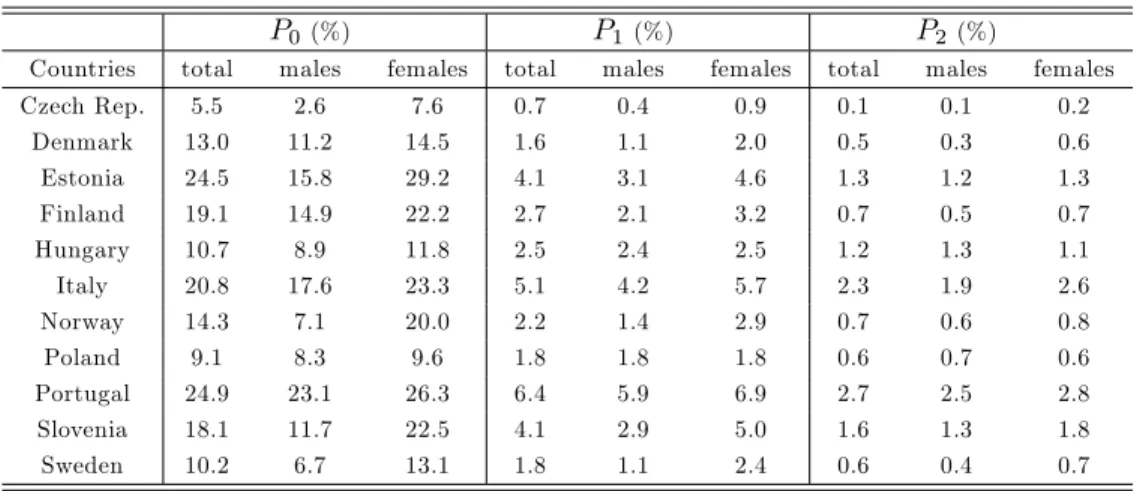
Given that the selection bias induced by income-di¤erentiated mortality is likely to be larger at higher ages, we will focus, throughout this section, on the measurement of old-age poverty, de…ned as poverty in the population aged 60 or more. The raw data on poverty in Europe in 2007 are presented in Table 1. Focusing …rst on simple headcount poverty measures, we see that the measured poverty at the old age varies strongly across countries. For instance, whereas only 5.5 % of the population aged 60 and more is below the poverty threshold in the Czech Republic, fractions as high as one fourth of the population aged 60 and more are below the poverty line in countries such as Estonia and

(17)

Portugal. Note also that, although women exhibit, in all countries under study, higher headcount poverty measures than men, the distribution of poverty across genders varies signi…cantly across countries. In some countries, such as Hungary or Poland, the proportion of persons in poverty at the old age is approximately the same for men and women. On the contrary, in countries like the Czech Republic or Norway, the poverty gap between women and men is much larger: the prevalence of poverty at the old age is, in those countries, about three times larger among women than among men.

If one now considers the extent of poverty, measured through the average income gap (P1) or squared income gap (P2), further observations can be made.

A …rst observation is that the ranking of countries in terms of poverty varies signi…cantly according to the FGT measure used. For instance, Norway exhibits a higher proportion of poor persons in the population in comparison to Hungary (14.3 % against 10.7 %), but the extent of poverty, as measured by the average income gap, is lower in Norway than in Hungary (2.2 % against 2.5 %).10 Fur-thermore, the size and sign of the poverty gender gap also varies with the FGT measure used. For instance, poverty among men is lower than among women in Poland when using headcount ratios, but the extent of poverty is larger among men than among women when focusing on the squared income gap.

P0(%) P1(%) P2(%)

Countries total males females total males females total males females Czech Rep. 5.5 2.6 7.6 0.7 0.4 0.9 0.1 0.1 0.2 Denmark 13.0 11.2 14.5 1.6 1.1 2.0 0.5 0.3 0.6 Estonia 24.5 15.8 29.2 4.1 3.1 4.6 1.3 1.2 1.3 Finland 19.1 14.9 22.2 2.7 2.1 3.2 0.7 0.5 0.7 Hungary 10.7 8.9 11.8 2.5 2.4 2.5 1.2 1.3 1.1 Italy 20.8 17.6 23.3 5.1 4.2 5.7 2.3 1.9 2.6 Norway 14.3 7.1 20.0 2.2 1.4 2.9 0.7 0.6 0.8 Poland 9.1 8.3 9.6 1.8 1.8 1.8 0.6 0.7 0.6 Portugal 24.9 23.1 26.3 6.4 5.9 6.9 2.7 2.5 2.8 Slovenia 18.1 11.7 22.5 4.1 2.9 5.0 1.6 1.3 1.8 Sweden 10.2 6.7 13.1 1.8 1.1 2.4 0.6 0.4 0.7

Table 1: FGT poverty measures at age 60+, for year 2007.11

Table 1 provides a contrasted picture of age poverty in Europe: old-age poverty levels vary across countries and gender, and are also sensitive to the FGT measure that is used. Note, however, that the picture provided by Table 1 may actually hide even larger discrepancies across European economies,

1 0_P1_{measures can be interpreted as follows: individuals whose income is below the poverty} line in e.g. Estonia have, on average, an income that is equal to 100 - 4.1 = 95.9 % of the poverty line. Regarding P2 measures, these can be interpreted as follows. Persons whose income is below the poverty line in e.g. Estonia have, on average, an income whose relative gap with respect to the poverty line raised to the power 2 is equal to 1.3 %.

(18)

which are related to di¤erentials in survival conditions across those countries. Di¤erential income-speci…c survival conditions across countries may, by leading to a more or less large number of "missing poor" - and a more or less large "hidden poverty" across those countries, distort the picture provided by Table 1. Those distortions due to di¤erent interferences caused by income-di¤erentiated mortality may concern the di¤erent FGT measures, to various extent.

In order to identify the impact of income-di¤erentiated mortality on poverty measurement, we need data on survival conditions by income levels. There is, to our knowledge, no lifetable by income for the European countries. However, Eurostat, produces comparable information on mortality by education.12 _To

il-lustrate the di¤erentials in life expectancy between and within countries, Tables 2 and 3 show, respectively, the life expectancy statistics at age 60 by gender, and by education level (primary, secondary and tertiary).13

Life expectancy at 60 Countries total men woman Czech Rep 20.8 18.5 22.7 Denmark 21.9 20.3 23.3 Estonia 19.7 15.9 22.5 Finland 23.3 20.8 25.6 Hungary 19.4 16.6 21.7 Italy 24.3 22.0 26.2 Norway 23.4 21.5 25.1 Poland 20.8 17.9 23.2 Portugal 23.1 21.0 25.1 Slovenia 22.2 19.4 24.5 Sweden 23.6 22.0 25.1

Table 2: Life expectancy at age 60 by gender 2007.

Life expectancy at 60 Countries primary secondary tertiary Czech Rep 20.68 20.38 23.55 Denmark 21.25 22.02 22.94 Estonia 16.53 20.25 22.76 Finland 22.91 23.45 24.30 Hungary 17.91 21.25 21.20 Italy 23.87 25.94 25.82 Norway 22.57 23.58 24.43 Poland 20.28 20.74 22.74 Portugal 23.06 23.58 24.04 Slovenia 21.86 22.13 23.43 Sweden 23.06 23.69 24.58

Table 3: Life expectancy at age 60 by education level, 2007.

1 2_{See: http://epp.eurostat.ec.europa.eu/portal/population/data/database.}

(19)

Table 2 shows the existence of signi…cant inequalities in longevity across Europe. The lowest life expectancy at age 60 is measured in Hungary (19.4 years), while the largest one is measured in Italy (24.3 years). Table 2 also highlights that the gender gap between women and men varies across countries, from 3 years in Denmark to 6.6 years in Estonia. However, as shown in Table 3, aggregate life expectancy statistics hide also large inequalities within countries, depending on the education level. The education gap in terms of life expectancy is very small is some countries, such as Sweden, where the life expectancy at age 60 for individuals with tertiary education is only 1.5 year larger than the one for individuals with primary education only. On the contrary, the education gap is much larger in Estonia, where it is equal to about 6.2 years.

The varying life expectancy gap across countries suggests that selection bi-ases in poverty measurement are likely to be varying across countries. In order to have a con…rmation of that conjecture, we need …rst to use the education-speci…c lifetables provided by Eurostat in order to extrapolate lifetables by income levels. For that purpose, we use a weighted ordinary least square re-gression, in line with Bossuyt et al (2004) and Van Oyen et al (2005). Taking into account the high correlation that exists between education and income, we can extrapolate mortality by income class on the basis of the mortality by education, by relating the distributions of individuals on both dimensions. For that purpose, we …rst transform the absolute educational status into a relative educational status. Indeed among cohorts, the size of educational groups has changed. Young people studied more than older ones. For a given cohort, we represent each category of education by its size in the population. We then order these categories from the lowest level to the highest on a scale from 0 to 100%. That is each category of income represents a percentage of the total pop-ulation of the cohort. This scale gives us a distribution of the cohort poppop-ulation according to education. We assume that the reference of an education category is determined by its relative position, de…ned as the mid-point of the proportion of the category represented on the ordered scale of 100% (Pamuk, 1985, 1988).14 We then regress the life expectancy by education on the reference mid-point of the education category by weighting for the prevalence of the category, i.e. the relative size of the educational level. The slope of the regression line represents the di¤erence in mortality between the bottom and the top of the education hierarchy. Once estimated, the coe¢ cients can be used to compute lifetables according to income. This is done by assuming that the social hierarchy given by the income is similar to the one given by education. We can thus apply the coe¢ cient of one education category to the corresponding categories of income. Figures 1 and 2 show, for the 11 European countries under study, the esti-mated life expectancy at age 60 by income class, for males and females respec-tively. For each country, life expectancy at age 60 is increasing with the income class considered. However, the longevity di¤erential related to income

inequal-1 4_{For example, if the …rst category is given by those with at most a primary degree and} represents 10% of the cohort, the mid-point reference will be 5%. If the second category represents, let’s say those with a secondary degree, 20% of the population, the bounds of the category in the distribution are 10 and 30% and the mid-point is 20%.

(20)

ity varies strongly across countries. The life expectancy di¤erential is especially large in Estonia and in the Czech Republic. On the contrary, it is much lower in Sweden and Denmark. Moreover, the life expectancy gap tends to be larger for males (Figure 1) than for females (Figure 2). The signi…cant variation in the size of the life expectancy gap in terms of income levels across countries and across gender implies that the selection bias in poverty measurement resulting from income-di¤erentiated mortality is likely to vary also across countries and gender. 10 15 20 25 10 15 20 25 10 15 20 25 0 20 40 60 80 100 0 20 40 60 80 100 0 20 40 60 80 100 0 20 40 60 80 100 0 20 40 60 80 100 0 20 40 60 80 100 0 20 40 60 80 100 0 20 40 60 80 100 0 20 40 60 80 100 0 20 40 60 80 100 0 20 40 60 80 100

Czech Denmark Estonia Finland

Hungary Italy Norway Poland

Portugal Slovenia Sweden

L if e exp ect an cy Income class

(21)

20 22 24 26 28 20 22 24 26 28 20 22 24 26 28 0 20 40 60 80 100 0 20 40 60 80 100 0 20 40 60 80 100 0 20 40 60 80 100 0 20 40 60 80 100 0 20 40 60 80 100 0 20 40 60 80 100 0 20 40 60 80 100 0 20 40 60 80 100 0 20 40 60 80 100 0 20 40 60 80 100

Czech Denmark Estonia Finland

Hungary Italy Norway Poland

Portugal Slovenia Sweden

Li fe e xpe cta ncy Income class

Figure 2: Life expectancy at age 60 by income class in Europe, females.

6.2 The adjustment technique

The adjustment of FGT poverty measures is made in two steps. First, we need to compute the number of "missing" persons for each country and each gender. Second, we need to assign a …ctitious income to those "missing persons".

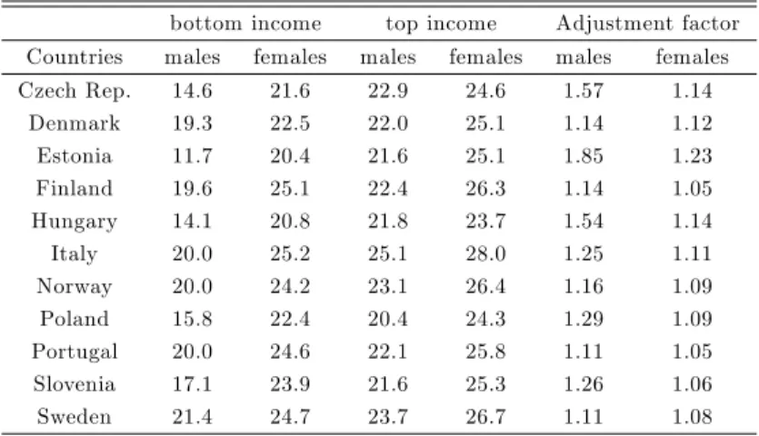
Regarding the …rst task, the number of "missing" individuals in each income class is computed, for each country and each gender, by calculating the hypo-thetical number of individuals of that class who would have survived if they had bene…ted from the survival conditions of the highest income class, for that coun-try and that gender. Assuming a stable demography, that number of "missing" individuals in an income class can be obtained by multiplying the number of surviving individuals in that class by a coe¢ cient equal to the ratio of income-speci…c life expectancies of the highest income class to the actual income class. As an illustration of that adjustment, Table 4 shows, for each country and each gender, the life expectancy statistics at age 60 for the bottom income class and for the top income class, as well as the corresponding adjustment coe¢ cient.

(22)

bottom income top income Adjustment factor Countries males females males females males females Czech Rep. 14.6 21.6 22.9 24.6 1.57 1.14 Denmark 19.3 22.5 22.0 25.1 1.14 1.12 Estonia 11.7 20.4 21.6 25.1 1.85 1.23 Finland 19.6 25.1 22.4 26.3 1.14 1.05 Hungary 14.1 20.8 21.8 23.7 1.54 1.14 Italy 20.0 25.2 25.1 28.0 1.25 1.11 Norway 20.0 24.2 23.1 26.4 1.16 1.09 Poland 15.8 22.4 20.4 24.3 1.29 1.09 Portugal 20.0 24.6 22.1 25.8 1.11 1.05 Slovenia 17.1 23.9 21.6 25.3 1.26 1.06 Sweden 21.4 24.7 23.7 26.7 1.11 1.08

Table 4: Life expectancy at age 60 for bottom and top income classes and the associated adjustment coe¢ cient, 2007.

Adjustment factors for the lowest income class are larger for males than for females, in line with the higher gaps in terms of life expectancy by income class. There is also a variation in adjustment factors across countries: these are large in Estonia and Czech Republic, but much smaller for Finland and Portugal.

Regarding the second task, which consists of assigning a …ctitious income to all those "missing" persons, we will, adopt two alternative approaches, which consists of two distinct matrices .15 _{The …rst approach consists of assigning, to}

each missing person, a …ctitious income equal to the income previously enjoyed. That approach consists of assuming that is an identity matrix. In that case, a premature death is, in some sense, treated as neutral for poverty measurement. Another, alternative approach, consists of counting a premature death as a source of deprivation, which leads to assign, as a …ctitious income, the income equivalent of death, that is, yN.

That welfare-neutral income, which makes an agent indi¤erent between, on the one hand, further life with that income, and, on the other hand, death, can be calibrated by following the work by Becker et al (2005). Taking income as a proxy for consumption, and assuming that individuals have time-additive preferences with a temporal utility function of the form u(y) = y_{1 1=}1 1= + , it is possible to derive the welfare-neutral income yN. yN makes the utility

associated to a life-period equal to the utility of being dead: y1 1=_N

1 1= + = 0 (13)

Following Becker et al (2005), we take = 1:25. Regarding the calibration of , we also follow Becker et al (2005), who use the estimation of " u_u(y)0(y)y = 0:346 from Murphy and Topel (2003) to extrapolate the level of . The value of " is estimated from compensating di¤erentials for occupational mortality risks;

(23)

it captures how individuals make trade-o¤ between more income and more risk. Then, for each country, we calculate the level of on the basis of the average income, while assuming = 1:25 and " = 0:346. Then, in a last stage, we compute, for each country, and on the basis of the parameters and (the former being country-speci…c), the level of the welfare-neutral income yN. Table

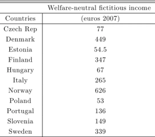
5 shows the values of the welfare-neutral income yN for each country.16

Welfare-neutral …ctitious income Countries (euros 2007) Czech Rep 77 Denmark 449 Estonia 54.5 Finland 347 Hungary 67 Italy 265 Norway 626 Poland 53 Portugal 136 Slovenia 149 Sweden 339

Table 5: Welfare-neutral income in Europe, 2007.

The welfare-neutral income yN is extremely low, which is not surprising.

Moreover, it varies strongly across countries, because of di¤erences in standards of living (i.e. the level of the average income in the country), which lead to di¤erent levels of the intercept . Those di¤erences may seem, at …rst glance, surprising. However, similar inequalities would be obtained under alternative calibration techniques using country-speci…c income and risk-taking attitudes.17

6.3 Results

Table 6 shows the adjusted FGT measures for poverty at age 60 and more obtained while assigning to each missing individual a …ctitious income equal to the past income enjoyed.18 _{In comparison with the unadjusted FGT poverty}

measures (Table 1), adjusted FGT measures are signi…cantly higher. Those higher levels re‡ect the inclusion, within all income classes, of the missing, prematurely dead, persons. Given that low income classes are also characterized by worse survival conditions - and thus require the addition of a larger number of missing persons -, low income classes include, proportionally, higher numbers

1 6_{Those …gures are expressed in yearly terms.}

1 7_{See, for instance, the meta-analysis made by Miller (2000) showing large di¤erentials in} the value of a statistical life across countries, depending on the income level.

1 8_{Throughout this section, the poverty line is assumed to keep the same level as before the} adjustment. That assumption is in line with the framework developed in Sections 2-5. Note that this assumption constitutes an obvious simpli…cation, since the addition of prematurely dead persons to the population may potentially a¤ect the level of the poverty line, and, hence, poverty measures. That e¤ect is discussed in Lefebvre et al (2013).

(24)

of added people than high income classes. Note, however, that, in theory, there was no obvious reason why FGT measures would necessarily be increased by the adjustment: this depends, in …ne, on whether the prematurely dead would have, in case of survival, su¤ered from a more severe poverty than the average surviving population. Table 6, when compared to Table 1, shows that adjusted poverty measures are unambiguously higher than unadjusted poverty measures.

^

P0(%) P^1(%) P^2(%)

Table 6: Adjusted FGT poverty measures at age 60+, for year 2007 (…ctitious income = past income).19

Note, however, that the extent of the adjustment varies signi…cantly across countries. The adjustment is very small in Sweden (+ 0.2 % for the headcount ratio), in Czech republic (+ 0.2 %), in Norway (+0.4 %) and in Finland (+ 0.4 %), but is much larger in countries such as Estonia (+ 1.7 % for the headcount ratio), Italy (+ 1.1 %) and Hungary (+1.0 %). This result re‡ects that the size of interferences induced by income-di¤erentiated mortality on poverty measures vary across countries. Another observation concerns the gender poverty gap. Table 6 suggests that, once poverty measures are adjusted, the gap between poverty prevalences among men and women is signi…cantly reduced. For in-stance, whereas the gender gap in Estonia was equal to 29.2 % - 15.8 % = 13.4 % in unadjusted terms (headcount), it is reduced to 31 % - 19.3 % = 11.7 % once poverty measures are adjusted. Hence the inclusion of the "missing persons" does not only a¤ect the overall poverty prevalence, but also lowers the gender poverty gap, even though women remain, on average, more subject to poverty.

In order to identify how the adjustment of poverty measures in‡uence the magnitudes of poverty across di¤erent FGT measures (i.e. for di¤erent values of ), Figure 3 shows the levels of the selection bias index under equal to 0, 1 and 2 (total population). The size of the selection bias induced by income-di¤erentiated mortality varies strongly across countries. Whereas it remains below 5 % in Denmark, Finland, Norway, Portugal, Slovenia and Sweden, the bias index reaches much higher levels in Estonia, Hungary and Poland.

(25)

Figure 3: Selection bias index for FGT measures, total population (…ctitious income =

past income)

Another important lesson from Figure 3 concerns the variation of the selec-tion bias index across FGT measures of poverty for a given country. At the theoretical level, there was no obvious clue regarding the behavior of the selec-tion bias index when varies. However, Figure 3 shows that, for the countries under study, the selection bias index tends to be higher for squared income gap measures ( = 2) than for average income gap measures ( = 1) and for headcount measures ( = 0). Hence, when the FGT poverty measure takes also into account the distribution of income, it is more subject to the selection bias induced by income-di¤erentiated mortality. Note that the extent to which the selection bias index increases with varies across countries. Those variations re‡ect the di¤erentials between income distributions across countries.

Let us now contrast those results with what is obtained under alternative …ctitious incomes. For that purpose, Table 7 shows the adjusted FGT poverty measures when the …ctitious income used for the extension of income pro…les of the prematurely dead persons consists of the welfare-neutral income yN. Note

that the income gap or the squared income gap is expected to be more sensitive to the level of …ctitious incomes than the headcount. The reason is that adopting the number 0 for all the poor made to survive or their past income that is below the poverty line has, by construction, the same impact on the headcount, but not on the income gap.

In the light of Table 7, several observations can be made. Firstly, the ad-justed FGT poverty measures take, under that alternative …ctitious income, much larger levels than when …ctitious incomes are equalized to past incomes. That result comes from the low levels of the welfare-neutral income yN (see

Ta-ble 5). Hence, when one considers premature death as a source of poverty and deprivation, and include it in poverty measures under the form of the income equivalent to death, poverty measures become much larger.

A second important point to be stressed concerns the strong di¤erentials across countries. The adjustment using the welfare-neutral income as a

(26)

…cti-tious income increases the old-age poverty rate (headcount) by 3.3 % in Denmark and by 4.1 % in Sweden (in comparison to the unadjusted poverty rate), but by 14 % for Estonia, and by 13.5 % in Czech Republic, and by 10.5 % in Hun-gary. Those large adjustments re‡ect the stronger di¤erentials in life expectancy across income classes in those countries (Figures 1 and 2).

^

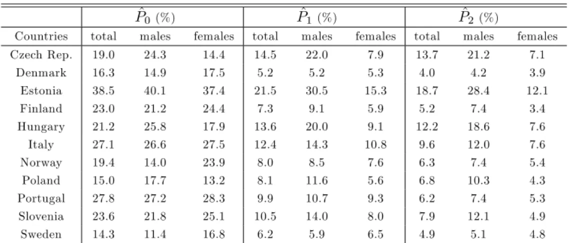
P0(%) P^1(%) P^2(%)

Table 7: Adjusted FGT poverty measures at age 60+, for year 2007 (…ctitious income = welfare-neutral income).20

A third observation concerns the size of the gender gap. Once the welfare-neutral income is used to extend the income pro…les of the prematurely dead, the form of the poverty gender gap is strongly altered in some countries. In Czech Republic, Estonia, Hungary and Poland, the headcount poverty measure is larger among men than among women, whereas the opposite was prevailing in unadjusted poverty measures. The reversal of the poverty gender gap observed in those countries is due to the fact that income-related di¤erentials in survival conditions are much larger among men than among women in those countries. Therefore, once the "missing" persons are added and are assigned yN as a

…cti-tious income, the poverty gender gap is reversed. Note that, in other countries, females remain, after the adjustment, more subject to poverty than men.

Finally, let us compute the selection bias index under that alternative ad-justment of FGT poverty measures (Figure 4). As we emphasized in Corollary 5, the selection bias index is, under a su¢ ciently low level of the welfare-neutral income, larger when using yN as a …ctitious income in comparison to the

ad-justment based on past incomes. The comparison of Figures 3 and 4 illustrates that corollary. The selection bias index takes larger values when the adjustment is based on the welfare-neutral, rather than on the past incomes. This re‡ects that the selection biases shown on Figures 3 and 4 have di¤erent informational contents. What the comparison of Figures 3 and 4 reveals is that the selection bias is much larger once one expects a poverty measure to take into account

(27)

not only the "missing poor" (as on Figure 3), but, also, the "missing poverty" (premature death being counted as a source of poverty).

Figure 4: Selection bias index for FGT measures, total population (…ctitious income =

welfare-neutral income)

Another important thing to be stressed is that, on Figure 4, the size of the selection bias index varies strongly across FGT poverty measures, and is much larger for squared poverty gap measures ( = 2) than for average poverty gaps ( = 1) and headcount ratios ( = 0). The size of the rise of the selection bias index when is increased is substantial, especially for countries such as Denmark, Finland, Norway, and Sweden. The intuition behind those larger increase in the selection bias index for those countries lies in the fact that the intensity of poverty in unadjusted terms is very low in those countries. Hence, given that unadjusted average poverty gap and squared poverty gap measures are low, the inclusion, within the income distribution, of the prematurely dead persons with very low incomes (equal to yN) generates a quite strong rise in

the intensity of poverty, in comparison to a low intensity in unadjusted terms. That rise is reinforced by the fact that poverty lines are much larger in those countries. Those larger poverty threshold lead to a higher intensity of poverty when the "missing persons" are added with a …ctitious income equal to the welfare-neutral income (which is much lower than the poverty line).

In the light of Figures 3 and 4, it appears that the noise or interferences caused by income-di¤erentiated mortality have di¤erent e¤ects on poverty mea-surement across classes of FGT measures and across countries. Eastern economies are characterized by larger income-related di¤erentials in survival conditions. Therefore, the adjustment strongly raises headcount poverty measures for those countries. On the contrary, Nordic economies su¤er from lower income-related di¤erentials in survival conditions, so that the number of "missing" persons is lower. This explains why Nordic economies exhibit lower selection bias indexes when = 0. However, for Nordic countries, the adjustment has a bigger impact on distribution-sensitive poverty indicators ( > 0), since these were very low

(28)

in unadjusted terms, and since the poverty line is larger in Nordic economies. Hence, once we take the intensity of poverty into account, Nordic countries exhibit selection bias indexes close to the ones of Eastern economies.

In sum, the selection bias induced by income-di¤erentiated mortality in a given economy varies depending on (1) the …ctitious incomes assigned to the prematurely dead persons; (2) the class of FGT poverty measure that is used. The determinant (1) plays a crucial role: when the …ctitious income assigned to the prematurely dead persons is equal to the welfare-neutral income, adjusted poverty measures are much larger than unadjusted poverty measures. But even for a given adjustment technique, there exist signi…cant variations in the selec-tion bias across the classes of FGT measures. Distribuselec-tion-sensitive measures are more subject to the selection bias than headcount measures. Furthermore, the present empirical section also highlights that the size of the selection bias varies strongly across countries. Those international di¤erentials - in particular the opposition between Nordic and Eastern Europe - mirror both international di¤erentials in income-related survival conditions and in the income distribution (including the level of the poverty line).

7 Concluding remarks

By mechanically reducing the proportion of poor persons in the population, income-di¤erentiated mortality introduces some noise in the measurement of poverty. This leads to the Mortality Paradox: a deterioration of the survival conditions faced by the poor can generate a decline in the measured poverty. That reduction is puzzling, and is a mere consequence of the absence of the "missing poor" in the population on which poverty is measured, and of the ignorance of premature death as a major aspect of poverty (Sen 1998).

This paper examined whether this puzzle for poverty measurement a¤ects FGT poverty measures. Our questions could be formulated as follows. Are FGT measures subject to the Mortality Paradox? If yes, are all subclasses of FGT measures equally subject to the Mortality Paradox?

To answer those questions, we developed a model of income mobility with risky lifetime to study how robust FGT measures are to variations in survival conditions. Robustness to mortality changes would make those measures immu-nized against the Mortality Paradox. We showed that the extent to which FGT measures are robust to changes in survival conditions depends on whether the prematurely dead would have, in case of survival, su¤ered from a more severe poverty than the average surviving population.

Under general conditions, such a robustness does not prevail. This moti-vated us to propose an adjustment of FGT measures, by extending the lifetime income pro…les of the prematurely dead, in line with Kanbur and Mukherjee (2007) and Lefebvre et al. (2013). Then, taking adjusted FGT measures with extended lifetime income pro…les as a benchmark, we identi…ed conditions under which the selection bias induced by income-di¤erentiated mortality is higher for distribution-sensitive measures than for headcount measures.

(29)

Finally, we illustrated that discussion by means of data on old-age poverty in 11 European economies (2007). The measured selection bias varies with the precise way in which we de…ne the adjusted poverty measure to which the unadjusted poverty measure is compared. Moreover, the selection bias induced by income-di¤erentiated mortality varies also across di¤erent subclasses of FGT measures. Those biases are lower for headcount measures than for measures taking the intensity of poverty into account. The size of the selection bias varies also across countries, depending on the shape of the income distribution, and on the severity of overmortality due to low income. Whereas Eastern European countries exhibit much larger selection biases than Nordic European countries under headcount measures, both Eastern and Nordic countries exhibit large selection biases when the intensity of poverty is also taken into account.

All in all, our exploratory study illustrates that the interferences caused by income-di¤erentiated mortality constitute a general problem for poverty mea-surement, that is, a problem concerns all subclasses of FGT measures and all countries (more or less advanced). Economies with large (unadjusted) poverty rates and strong overmortality for the poor are concerned by the selection bias. But more surprisingly, distribution-sensitive poverty measures for richer economies with little income-di¤erentiated mortality are also subject to selection biases. The reason is that, in their case, taking the "missing poor" and the "hid-den poverty" into account creates a much bigger contrast with the standards of the surviving populations. Hence, even when considering rich economies, distribution-sensitive poverty measures are not immunized against selection bi-ases due to income-di¤erentiated mortality.

8 References

Backlund, E., Sorlie, P. & Johnson, N. (1999) A comparison of the relationships of education and income with mortality: the national longitudinal mortality study. Social Science and Medicine, 49 (10): 1373-1384.

Bossuyt N, Gadeyne S, Deboosere P,Van OyenH (2004) Socio-economic inequalities in healthy expectancy in Belgium. Public Health 118:3–10

Deaton, A. & Paxson, C. (1998) Aging and inequality in income and health. American Economic Review, 88: 248-253.

Deaton, A. (2003) Health, inequality and economic development. Journal of Economic Literature, 41: 113-158.

Duggan, J., Gillingham, R. & Greenlees, J. (2007) Mortality and lifetime income: evidence from U.S. Social Security Records. IMF Working Paper, 07/15.

Duleep, H.O. (1986) Measuring the e¤ect of income on adult mortality using longitudinal administrative record data. Journal of Human Resources, 21 (2): 238-251.

Foster, J., Greer, J. & Thorbecke, E. (1984) A class of decomposable poverty measures. Econometrica, 52 (3): 761-766.

Jusot, F. (2004): Mortalité et revenu en France: construction et résultats d’une enquête cas-témoins. Santé, Société et Solidarité, 3 (2): 173-186.

(30)

Kanbur, R. & Mukherjee, D. (2007) Premature mortality and poverty measurement. Bul-letin of Economic Research, 59 (4): 339-359.

Lefebvre, M., Pestieau, P. & Ponthiere, G. (2013) Measuring Poverty Without the Mor-tality Paradox. Social Choice and Welfare, 40 (1): 285-316.

Miller, T. (2000) Variations between countries in values of statistical life. Journal of Transport Economics and Policy 34 (2): 169-188.

Murphy, K. & Topel, R. (2003) The Economic value of medical research. In: K. Murphy and R. Topel (eds.): Measuring the Gains from Medical Research: An Economic Approach. The University of Chicago press.

Pamuk ER (1985) Social class inequality in mortality from 1921 to 1972 in England andWales. Popul Stud, 39:17–31

Pamuk ER (1988) Social class inequality in infant mortality in England and Wales from 1921 to 1980. Eur J Popul 4:1–21

Salm, M. (2007) The e¤ect of pensions on longevity: evidence from Union Army veterans. IZA Discussion Paper 2668.

Sen AK (1998) Mortality as an indicator of economic success and failure. Econ J 108:1–25 Snyder, S. & W. Evans (2006) The e¤ect of income on mortality: evidence from the social security notch. Review of Economics and Statistics, 88 (3): 482-495.

Van Oyen H, Bossuyt N, Deboosere P, Gadeyne S, Abatith E, Demarest S (2005) Di¤er-ential inequity in health expectancy by region in Belgium. Soc Prev Med 50(5):301–310