HAL Id: tel-02063268
https://tel.archives-ouvertes.fr/tel-02063268
Submitted on 11 Mar 2019
HAL is a multi-disciplinary open access archive for the deposit and dissemination of sci-entific research documents, whether they are pub-lished or not. The documents may come from teaching and research institutions in France or abroad, or from public or private research centers.
L’archive ouverte pluridisciplinaire HAL, est destinée au dépôt et à la diffusion de documents scientifiques de niveau recherche, publiés ou non, émanant des établissements d’enseignement et de recherche français ou étrangers, des laboratoires publics ou privés.
Sparse representations in vibration-based rolling element
bearing diagnostics
Ge Xin
To cite this version:
Ge Xin. Sparse representations in vibration-based rolling element bearing diagnostics. Vibrations [physics.class-ph]. Université de Lyon, 2017. English. �NNT : 2017LYSEI051�. �tel-02063268�
N°d’ordre NNT : 2017LYSEI051
THESE de DOCTORAT DE L’UNIVERSITE DE LYON
opérée au sein de
l’INSA LYON
Ecole Doctorale
N° 162MECANIQUE, ENERGETIQUE, GENIE CIVIL, ACOUSTIQUE
Spécialité/ discipline de doctorat
: AcoustiqueSoutenue publiquement le 22/06/2017, par :
Ge XIN
Sparse Representations in
Vibration-based Rolling Element Bearing
Diagnostics
Devant le jury composé de :
CHIEMENTIN Xavier, Maître de Conférences – HDR, URCA Rapporteur CORBIER Christophe, Maître de Conférences – HDR, Université de Lyon Rapporteur DRON Jean-Paul, Professeur des Universités, URCA Examinateur KAFTANDJIAN Valérie, Professeur des Universités, INSA-Lyon Examinatrice ANTONI Jérome, Professeur des Universités, INSA-Lyon Directeur de thèse HAMZAOUI Nacer, Professeur des Universités, INSA-Lyon Co-directeur de thèse
Sparse Representations in
Vibration-based Rolling Element
Bearing Diagnostics
Ge XIN
Laboratoire Vibrations Acoustique
INSA-Lyon
This dissertation is submitted for the degree of
Doctor of Philosophy
I would like to dedicate this thesis to my loving parents, my dear wife and my cute daughter Yucheng.
Acknowledgements
This thesis has been made possible thanks to the generous help of many people, and I wish to offer my most heartfelt thanks to them.
First and foremost, I would like to thank my supervisors, Prof. Jérôme Antoni and Prof. Nacer Hamzaoui. Thanks for giving me this excellent opportunity to work on this exciting project. It has been an exceptional privilege to work with such kind, insightful, energetic, and knowledgeable advisers. Jérôme, no words can express my appreciation for your outstanding support, relentless encouragement and unwavering guidance throughout my academic career. Along all these, I understand such famous expression: “If I have seen further, it is by standing on the shoulders of giants” and for all these my deepest gratitude goes to you. Nacer, you are the most enthusiastic person I have ever met. Your patience, enthusiasm and kindness always inspire me to think positive and overcome any difficulty. Once again, I sincerely thank you. I specially express my thanks to Dr. Xavier Chiementin and Dr. Christophe Corbier for reviewing this manuscript and Prof. Jean-Paul Dron and Prof. Valérie Kaftandjian for accepting as the jury of my thesis.
I would like to thank all my colleagues in the laboratory for their help during my stay in France. My thanks go especially to Dr. Liang Yu, who provided me many valuable scientific suggestions. Prof. Erliang Zhang and Dr. Bin Dong who gave me a lot of advice and shared their experiences. I miss the time spent with Edouard Cardenas Cabada, Souhayb Kass, Philéas Maigrot, Edgar Sierra Alonso, Marco Buzzoni and Charles Vanwynsberghe, who gave me warm encouragement and generous assistance. I would like to extend my thanks to many friends in Lyon, Emmanuel Roux, Inés Mérida, Corinne Lotto, Fulbert Mbailassem and Ting Su. We passed so much wonderful time together.
I would also show my gratitude to China Scholarship Council (CSC) for the financement and Laboratoire Vibrations Acoustique (LVA) for the support during my Ph.D. study.
Finally, my sincere thanks go to my family for their unconditional love and support in everything I do. Thanks my parents and my parents-in-law for taking care of my daughter and helping us to go through a very difficult time in our life. To my beloved wife, Miaomiao, thanks for your love and being there in my life. To my daugther, Yucheng, thanks for always making me feel like the happiest dad in the world.
Abstract
Although vibration-based rolling element bearing diagnostics is a very well-developed field, the research on sparse representations of vibration signals is yet new and challenging for machine diagnosis. As a desired property – representation of a signal in highly organized structure – sparsity enables us to reveal the natural signature of singular events embedded in a signal so as to reduce the demand on the user’s expertise, even though it involves advanced theory of stochastic processes. In this thesis, several novel methods have been developed, by means of different stochastic models, associated with their effective algorithms so as to serve the industry in rolling element bearing diagnostics.
First, the sparsity-based model (sparse code, in natural image processing) is investigated based on the current literature. By summarizing its successful reasons from three points, the historical background of sparse representations has been inquired in the field of natural scenes. Along such three aspects, its mathematical model with corresponding algorithms has been categorized and presented as a fundamental premise; the main publications are therefore surveyed in the literature on machinery fault diagnosis; finally, by discussing the pros and cons of sparse representations, an interpretation of sparse structure in the Bayesian viewpoint is proposed which then gives rise to two novel models for machinery fault diagnosis.
Second, a new stochastic model is introduced to address this issue: it introduces a hidden variable to indicate the occurrence of the impacts and estimates the spectral content of the corresponding transients together with the spectrum of background noise. This gives rise to an automatic detection algorithm – with no need of manual prefiltering as is the case with the envelope spectrum – from which fault frequencies can be revealed. The same algorithm also makes possible to filter out the fault signal in a very efficient way as compared to other approaches based on the stationary assumption. The performance is investigated on synthetic signals with a high noise-to-signal ratio and also in the case of a mixture of two independent transients. The effectiveness and robustness of the method are also verified on vibration signals measured on a test-bench (gears and bearings). Results are found superior or at least equivalent to those of conventional envelope analysis and fast kurtogram.
Third, a novel scheme for extracting cyclostationary (CS) signals is proposed. It in-troduces a periodic-variance based stochastic model to recover the CS component in the
masking of interfering signals. This proceeds from the property that, for a CS signal, the STFT evidences periodic flows of energy in and across its frequency bins. By considering the periodic variance as hidden variables, a time-varying filter is designed so as to achieve the full-band reconstruction of CS signals characterized by some pre-set characteristic frequency, which can be obtained by the prior knowledge or the estimator of Spectral Correlation. The performance of the proposed scheme has been demonstrated on synthetic and experimental cases. Of particular interest is the robustness on experimental data sets and superior extraction capability over the conventional Wiener filter. It not only deals with the bearing fault at an incipient stage, but it even works for the installation problem and the case of two sources, i.e. bearing and gear faults together. Eventually, these experimental examples evidence its versatile usage on diagnostic analysis of compound signals.
Fourth, a benchmark analysis by using the fast computation of the spectral correlation is provided. This study benefits from a big data set – which is publicly available and widely used – supplied by the Case Western Reserve University (CWRU) Bearing Data Center. Particularly, it contains plenty of cases ranges from very easily diagnosable to not diagnosable; while some signals are showing the typical harmonic structure of bearing fault signatures, others are quite blurry or even display other fault symptoms. This is one crucial point that makes this work challenging and charming – moving forward the benchmark study of the CWRU data set – by uncovering its own unique characteristics.
Résumé
Bien que le diagnostic des roulements par analyse vibratoire soit un domaine très développé, la recherche sur les représentations parcimonieuses des signaux de vibration est encore nou-velle et difficile pour le diagnostic des machines tournantes. En tant que propriété souhaitée – la représentation d’un signal dans une structure hautement organisée – la parcimonie nous permet de révéler la signature naturelle d’événements singuliers intégrés dans un signal afin de réduire la demande sur l’ expertise de l’ utilisateur, même si elle implique une théorie avancée des processus stochastiques. Dans cette thèse, de méthodes nouvelles ont été développées, au moyen de différents modèles stochastiques, associées à des algorithmes efficaces afin de servir l’industrie dans le diagnostic des roulements.
Tout d’abord, les modèles parcimonieux présentés dans la littérature sont revus. En résumant leurs avantages en trois points, le contexte historique des représentations parci-monieuses a été examiné, notamment dans le domaine des scènes naturelles. En suivant ces trois aspects, les modèles mathématiques ainsi que les algorithmes associés ont été classés et présentés comme une prémisse fondamentale. Les principales publications concernant le diagnostic des machines tournantes ont également été considérées. Enfin, en discutant des avantages et des inconvénients des représentations parcimonieuses, une interprétation des structures creuses d’un point de vue Bayésien est proposée, ce qui donne lieu à deux nouveaux modèles de diagnostic des machines tournantes.
Dans un second temps, un nouveau modèle stochastique est proposé : il introduit une variable cachée relative à l’apparition d’impacts et estime le contenu spectral des transitoires correspondants ainsi que le spectre du bruit de fond. Cela donne lieu à un algorithme de détection automatique - sans besoin de pré-filtrage manuel comme c’est le cas avec le spectre d’enveloppe - à partir duquel les fréquences de défaut peuvent être révélées. Le même algorithme permet également de filtrer le signal de défaut de manière très efficace par rapport à d’autres approches basées sur l’hypothèse stationnaire. La performance de l’algorithme est étudiée sur des signaux synthétiques avec un rapport signal à bruit faible et également dans le cas d’un mélange de deux transitoires indépendants. L’efficacité et la robustesse de la méthode sont également vérifiées sur les signaux de vibration mesurés sur un banc
d’essai (engrenages et paliers). Les résultats sont meilleurs ou au moins équivalents à ceux de l’analyse d’enveloppes classique et du kurtogramme rapide.
Dans un troisième temps, un nouveau schéma pour l’extraction de signaux cyclo-stationnaires (CS) est proposé. Il introduit un modèle stochastique basé sur la variance périodique pour récupérer la composante CS masquée par des signaux parasites. Cela dé-coule de la propriété statuant que, pour un signal CS, la transformée de Fourier à court terme met en évidence des flux d’énergie temporellement périodiques. En considérant la variance périodique en tant que variable cachée, un filtre temporel est conçu de manière à obtenir la reconstruction intégrale des signaux CS caractérisés par une fréquence cyclique préétablie, qui peut être connue à priori ou estimée à partir de la corrélation spectrale. La performance du schéma proposé a été évaluée sur des cas synthétiques et expérimentaux. Un intérêt particulier de la méthode est sa robustesse lorsqu’elle est appliquée sur des données expérimentales ainsi qu’une capacité d’extraction supérieure par rapport au filtre de Wiener conventionnel. Cette approche se révèle efficace non seulement sur des défauts de roulement à des stades précoces, mais également sur des problèmes de montage dans le cas où plusieurs sources sont présentes (par exemple les engrenages et les roulements ensemble). Finalement, ces exemples expérimentaux témoignent de l’utilisation polyvalente de la méthode à des fins de diagnostic de signaux composés.
Pour finir, une analyse comparée utilisant le calcul rapide de la corrélation spectrale est réalisée sur une base de données publiquement disponible et largement utilisée. Cette base bénéficie d’un grand ensemble de données fournies par le centre de données de l’Université Case Western Reserve (CWRU). En particulier, elle contient de nombreux cas d’étude, allant de diagnostics simples aux plus complexes. Tandis que certains signaux présentent une structure harmonique typique des signatures de défauts de roulement, d’autres sont assez ambigües ou présentent d’autres symptômes inattendus de défaut. C’est un point crucial qui fixe un défis non-trivial à resoudre.
Table of contents
List of figures xv List of tables xxv 1 Introduction 1 1.1 Context . . . 1 1.2 Problem statement . . . 31.3 State of the art . . . 5
1.4 Focus and Contribution . . . 6
1.5 Outline . . . 8
2 Literature review on sparse representations of vibration signal 9 2.1 Derivation of sparse code . . . 9
2.2 Sparsity-based models . . . 11
2.2.1 Synthesis model . . . 13
2.2.2 Analysis model . . . 14
2.2.3 Comparison and evolution . . . 14
2.3 Algorithms for sparse representation . . . 15
2.3.1 Sparse coding . . . 16
2.3.2 Learning-based dictionary . . . 17
2.4 Applications on rolling element bearing diagnostics . . . 18
2.5 Discussion and conclusion . . . 21
3 Automatic Spectrum Matching of Repetitive Transients Based on Hidden Markov Model 25 3.1 Spectral mixture model . . . 25
3.1.1 Model and assumption . . . 26
3.1.2 Hidden Markov model . . . 27
3.2 Reconstruction scheme for repetitive transients . . . 33
3.3 Parameter selection . . . 35
3.3.1 Initial settings . . . 35
3.3.2 Cases 1 & 2: demonstration of parameter selection . . . 38
3.3.3 Case 3: Comparison of different spectral correlation assumptions . 42 3.3.4 Case 4: diagnostics and separation of a mixture of independent transients . . . 47
3.4 Validation on vibration signals . . . 51
3.4.1 Case 5: diagnosis of a ball fault . . . 51
3.4.2 Cases 6 & 7: diagnostics of bearing and gears . . . 57
3.4.3 Case 8: diagnostics of bearing in nonstationary regime . . . 62
3.4.4 Case 9: diagnosis in the presence of multiple components . . . 67
3.5 Conclusion . . . 72
4 Extraction of cyclostationary signals 73 4.1 Periodic-variance based model . . . 73
4.1.1 Model and assumptions . . . 73
4.1.2 Periodic-variance based model . . . 74
4.2 Extraction scheme for cyclostationary signals . . . 76
4.3 Parameter selection . . . 79
4.3.1 Initial settings . . . 79
4.3.2 Cases 1 & 2: demonstration of parameter selection . . . 81
4.4 Validation on experimental examples . . . 89
4.4.1 Example 1: extraction of bearing signals with good gears . . . 89
4.4.2 Example 2: separation of bearing signals with broken gears . . . . 103
4.5 Conclusion . . . 113
5 Benchmark survey on using the fast spectral correlation 115 5.1 Background on applied diagnostic methods . . . 115
5.2 Case Western Reserve University data . . . 118
5.2.1 Experimental set-up . . . 121
5.2.2 Examples and discussion . . . 121
5.3 Result tables and conclusion . . . 130
6 Conclusions and perspectives 133 6.1 Conclusions . . . 133
Table of contents xiii
References 137
Appendix A Commonly used symbols and statistical quantities 145 Appendix B Proof of the mixture distribution with two Gaussian distributions
giving rise to a super-Gaussian distribution 149 Appendix C Proof of the inverse gamma distribution giving rise to a conjugate
prior for the variance 151 Appendix D Tables of results 153
List of figures
1.1 Typical fault signals in rolling element bearings. . . 2
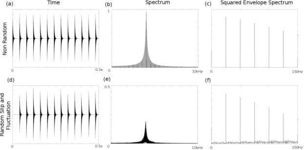
1.2 Illustration of the influence of random slips and fluctuations: (a) and (d) stand for synthetic signals in time domain; (b) and (e) for raw spectra calculated by the Fourier transform; (c) and (f) for squared envelope spectra. . . 4
2.1 (Fig.1 in Ref. [35]) Sparse coding. (a) An image is represented by a small number of “active” code elements, ai, out of a large set. Which elements
are active varies from one image to the next. (b) Since a given element in a sparse code will most of the time be inactive, the probability distribution of its activity will be highly peaked around zero with heavy tails. This is in contrast to a code where the probability distribution of activity is spread more evenly among a range of values (such as a Gaussian). . . 10
2.2 (Table 1.1 in [37]) Some robust penalty functions. For all cases, C(γ) = ∑iρ(γi). . . 13
2.3 Graphical illustration of the synthesis model, which represents a sparse vibration signal as a linear combination of three actived atoms in Dictionary. As can be seen, noisy measurements in blue, reconstructed signal in red, reference signal in green, actived atoms in black. It is notice that not all the atoms are displayed in the block of Dictionary, alternatively, only ten identifiable waveforms of trained atoms are displayed. . . 14
2.5 Illustration of Spectral Kurtosis analysis: the repetitive series of transients passes a filter-bank analysis implemented by the STFT; as can be seen in Ky( fb), there exist two different distributions which indicate the fault
com-ponent (centered at frequency f1) and the noisy component (centered at
frequency f0), respectively. It is highlighted that along the time instant the
occurrence of transients can be characterized by means of a latent variable (i.e. the spectral mixture model in Chapter 3). In particular, for cyclostation-ary singals, its energy flow displays a periodical variation which indicates cyclostationarity in second-order statistics (i.e. the periodic-variance based model in Chapter 4). . . 23
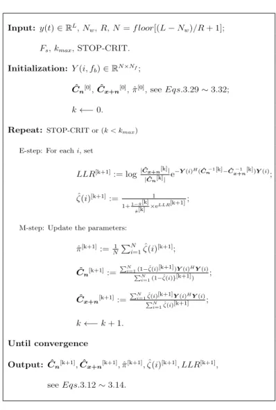
3.1 Explicit steps of the EM algorithm to infer the parameters in the HMM. . . 30 3.2 Graphical model in the case K= 2. . . 32 3.3 Illustration of how to select the window length Nwand shift R with respect
to transient durations TI and cycle ∆t. . . 36
3.4 Spectrogram of the signal simulated in Case 1 with resonance frequency f0 = 0.15 Hz, r = 0.95 and fault frequency α0= 1.25× 10⁻³ Hz (T =
1/α0= 800 s, Nw= 27and R= 20). . . 38
3.5 (a) Synthetic signal of Case 1 with white noise (noise-to-signal-ratio= 6 dB. (b) Synthetic repetitive transients. (c) Initialized latent variable ˆζ(i)[0] (black line) with threshold (red dotted line) set to 0.01max( ˆζ(i)[0]) with
ˆ
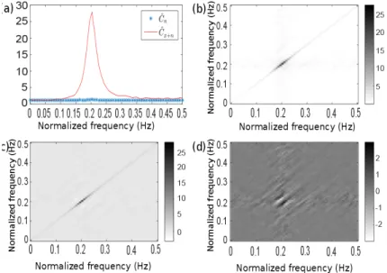
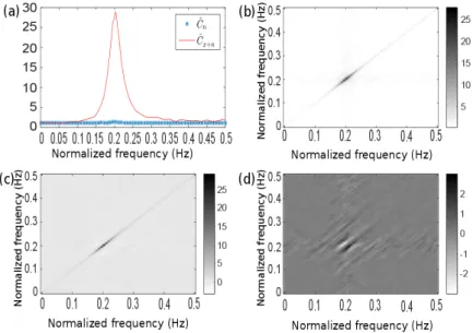
π[0]= 0.112. (d) Estimated latent variable ˆζ(i). . . 39 3.6 (a) Initialized spectra (diagonals of covariance matrices ˆCCC[0]nnn and ˆCCC[0]xxx (red line
and blue asteriks) and (b) estimated ones from EM (diagonals of covariance matrices ˆCCC[k+1]nnn and ˆCCC[k+1]xxx (red lines) together with the theoretical frequency response H(z) (black dashed line and blue asteriks). . . 40 3.7 (a) LLR and (b) latent variable ˆζ(i) in the time domain. . . 40 3.8 Spectrogram of the signal simulated in Case 2 with resonance frequency
f0= 6× 10⁻³ Hz, r= 0.9 and fault frequency α0= 1.25× 10⁻³Hz. . . 41
3.9 Spectra of the LLR (a) and of the latent variable (b) presented in Fig. 3.7 together with the SES of actual fault signal (red dotted line). The limit αmax=
7.8× 10⁻³ Hz is indicted by a vertical black dotted line (Normalization to unit maximum value). . . 41 3.10 Spectrogram of the signal simulated in Case 3 with resonance frequency
List of figures xvii
3.11 Spectra of the LLR together with the theoretical SES (red dotted line) (a) full matrix, (b) diagonal matrix, (c) tridiagonal matrix, (d) low rank matrix, (e) Toeplitz matrix (normalization to unit maximum value). . . 43 3.12 Spectra of the latent variable ˆζ(i) together with the theoretical SES (red
dotted line) (a) full matrix, (b) diagonal matrix, (c) tridiagonal matrix, (d) low rank matrix, (e) Toeplitz matrix (normalization to unit maximum value). 43 3.13 Full matrix: (a) diagonals (the spectrum of the fault signal is indicated by a
red solid line and that of the noise by blue asterisks); (b) absolute value; (c) real part; (d) imaginary part of the estimated covariance matrix. . . 44 3.14 Diagonal matrix: (a) diagonals (the spectrum of the fault signal is indicated
by a red solid line and that of the noise by blue asterisks); (b) absolute value; (c) real part; (d) imaginary part of the estimated covariance matrix. . . 45 3.15 Tridiagonal matrix: (a) diagonals (the spectrum of the fault signal is indicated
by a red solid line and that of the noise by blue asterisks); (b) absolute value; (c) real part; (d) imaginary part of the estimated covariance matrix. . . 45 3.16 Low rank matrix: (a) diagonals (the spectrum of the fault signal is indicated
by a red solid line and that of the noise by blue asterisks); (b) absolute value; (c) real part; (d) imaginary part of the estimated covariance matrix. . . 46 3.17 Toeplitz matrix: (a) diagonals (the spectrum of the fault signal is indicated
by a red solid line and that of the noise by blue asterisks); (b) absolute value; (c) real part; (d) imaginary part of the estimated covariance matrix. . . 46 3.18 (a) Component XXX1(i) with period T1= 530 samples (στ1= 0.02T1and σ
1 A=
0.1). (b) Component XXX2(i) with period T2= 470 samples (στ2= 0.02T2and
σA2= 0.1). (c) Noisy measurement (noise-to-signal ratio = 0 dB). . . 47 3.19 Spectrogram of the signal simulated in Case 4 with two components (T1=
530 samples and T2= 470 samples respectively). . . 48
3.20 Estimated spectra of component XXX1(i) (red solid line), component XXX2(i) (green solid line) and noise (blue dashed line). The two theoretical frequency responses of H(z) are indicated by black dashed lines. . . 48 3.21 (a) Estimated latent variable ζ1(i) (red solid line) together with the actual
first component (black solid line). (b) Estimated latent variable ζ2(i) (green solid line) together with the actual second component (black solid line). . . 49 3.22 Spectra of the estimated latent variable (a) ζ1(i) and (b) ζ2(i) (normalized
3.23 Reconstructed repetitive transients corresponding to (a) the first component X
XX1(i) with period T1= 530 samples and (b) the second component XXX2(i)
with period T2= 470 samples. (c) Summation of two components XXX1(i) and
X
XX2(i). . . 50 3.24 Spectrogram (logarithmic scale) of signal of Case 5 (frequency resolution
∆ f = 375 Hz). . . 52 3.25 SES of the raw signal (normalized to unit maximum value). . . 53 3.26 Diagonals of covariance matrices (frequency resolution ∆ f = 375 Hz); the
spectrum of the fault signal is indicated by a red solid line and that of the noise by a blue dashed line. . . 53 3.27 Spectrum of the LLR with markers at the theoretical fault frequency and
harmonics; the limit αmax = 375 Hz is indicted by a vertical black dotted
line (normalization to unit maximum value). . . 54 3.28 Kurtogram of signal of Case 5 computed over K= 7 levels with a 1/3-binary
tree and an 8 coefficient prototype filter. Several local maxima are presented. One relevant maximum is found at dyad{ f10;(∆ f )4} = {14250; 1500} Hz. 55
3.29 SES in frequency band[13500; 15000] Hz returned by the kurtogram (nor-malization to unit maximum value). . . 55 3.30 (a) Vibration signal of Case 5 and (b) its band-pass filtered version in the
frequency band[13500; 15000] Hz. (c) Full-band reconstructed fault signal from the proposed HMM-based time-varying filter. . . 56 3.31 (a) Enlarged view of vibration signal of Case 5 (with indication of the period
corresponding to the peak fg in Fig. 3.25) and (b) enlarged view of its
band-pass filtered version in the frequency band [13500; 15000] Hz. (c) Enlarged view of the full-band reconstructed fault signal from the proposed HMM-based time-varying filter. . . 57 3.32 Test rig setup. . . 58 3.33 Spectrum of the LLR with markers at the suspected fault frequency BPFO
and its harmonics (normalization to unit maximum value). . . 59 3.34 Fast kurtogram of signal of Case 6 computed over K= 7 levels with a
1/3-binary tree and an 8 coefficient prototype filter. One relevant maximum is found at dyad{ f13;(∆ f )4} = {20k; 1600} Hz. . . 60
3.35 SES of complex envelope in dyad { f13;(∆ f )4} = {20k; 1600} Hz
corre-sponding to the frequency band [18400; 21600] Hz with markers at the suspected fault frequency BPFO and its harmonics (normalization to unit maximum value). . . 60
List of figures xix
3.36 (a) Vibration signal of Case 6 in time interval[1.9 2.3] s and (b) its band-pass filtered version in frequency band [18400; 21600] Hz. (c) Reconstructed transients from the HMM-based time-varying filter. . . 61 3.37 Spectrum of the LLR with markers at the suspected fault frequencies BPFO,
its harmonics and f(rot,2) (normalization to unit maximum value). . . 62 3.38 (a) Estimated instantaneous speed of signal in Case 8 and (b) its
corre-sponding acceleration signal which undergoes speed-dependent magnitude modulation. (c) Division of the estimated instantaneous speed in 5 regimes. 63 3.39 (a) Raw signal in regime No. 1 and (b) the corresponding reconstructed
transients from the HMM-based time-varying filter. . . 64 3.40 (a) Raw signal in regime No. 2 and (b) the corresponding reconstructed
transients from the HMM-based time-varying filter. . . 64 3.41 (a) Raw signal in regime No. 3 and (b) the corresponding reconstructed
transients from the HMM-based time-varying filter. . . 65 3.42 (a) Raw signal in regime No. 4 and (b) the corresponding reconstructed
transients from the HMM-based time-varying filter. . . 65 3.43 (a) Raw signal in regime No. 5 and (b) the corresponding reconstructed
transients from the HMM-based time-varying filter. . . 66 3.44 Order spectrum of the LLR with markers at the suspected fault frequency
BPOO and its harmonics (normalization to unit maximum value). . . 66 3.45 Measured signal (a) from 0 to 2.5 s and (b) from 2.5 to 5 s which evidence
of instantaneous interfering component in time interval[3.4 4] s. . . 68 3.46 Spectrogram (logarithmic scale) of signal in time intervals (a)[1.9 2.3] s and
(b)[3.45 3.85] s of Case 9 with evidence of two states: a global distribution with spectral content in band [1.8 3.8] kHz and a local distribution with spectral content in band[1.8 3.8] kHz and [9 11] kHz. . . 69 3.47 Diagonals of the covariance matrices of the three components, XXX1(i) (red
solid line), XXX2(i) (green solid line) and noise (blue dashed line). . . 69 3.48 Spectra of the estimated latent variable (a) ζ1(i) and (b) ζ2(i), respectively
(normalization to unit maximum value). . . 70 3.49 (a) Measured signal from 3.45 to 3.85 s. Reconstructed components (b) XXX1(i)
and (c) XXX2(i) from the HMM-based time-varying filter. . . 70 3.50 (a) Measured signal from 1.9 to 2.3 s. Reconstructed components (b) XXX1(i)
4.1 Spectrogram of the signal simulated in Case 1 with resonance frequency f0= 0.1 Hz, r = 0.95 and fault frequency α0= 5× 10⁻³ Hz (T = 1/α0=
000 s, Nw= 25and R= 4). . . 82
4.2 (a) Synthetic signal of Case 1 with white noise (noise-to-signal-ratio= 6 dB. (b) Synthetic transient signal. (c) Recovered time signal ˆx[n]. . . 83 4.3 (a) Initialized time-dependent variance of the CS signal, ˆσx2(i; fb)[0], and
(b) the estimated ˆσx2(i; fb)[k+1]from the EM algorithm. (c) Spectrogram of
the estimated CS signal, bX(i, fb), with (d) its periodic time-varying filter
1/(1 + H(i; fb)) as defined in Eqs. 4.15-4.16. . . 83
4.4 (a) Initialized spectra (variance of noise and CS signals ˆσn2( fb)[0]and ˆσx2( fb)[0],
in blue dotted line and red line, respectively) and (b) estimated spectra from the EM algorithm, ( ˆσn2( fb)[k+1]and ˆσx2( fb)[k+1], in blue dotted line and red
line, respectively) together with the theoretical squared magnitude frequency response|H(z)|2(black dashed line). . . 84 4.5 Cyclostationary index: function of the frequency fbby means of taking the
standard deviation of ˆσx2(i; fb)[k+1]over the time instant i. . . 85
4.6 (a) Enlarged view of the recovered time signal ˆx[n] of Fig. 4.2 (b) and (c). (b) Initialized time-dependent variance of the CS signal, ˆσx2(i; fb)[0], and (c)
the estimated ˆσx2(i; fb)[k+1]from the EM algorithm. . . 85
4.7 (a) Synthetic signal of Case 2 with white noise (noise-to-signal-ratio= 6 dB. (b) Synthetic repetitive transient signal. (c) Recovered time signal ˆx[n]. . . . 86 4.8 (a) Initialized time-dependent variance of the CS signal, ˆσx2(i; fb)[0], and
(b) the estimated ˆσx2(i; fb)[k+1]from the EM algorithm. (c) Spectrogram of
the estimated CS signal, bX(i, fb), with (d) its periodic time-varying filter
1/(1 + H(i; fb)) as defined in Eqs. 4.15-4.16. . . 87
4.9 (a) Enlarged view of the recovered time signal ˆx[n] of Fig. 4.7 (b) and (c). (b) Initialized time-dependent variance of the CS signal, ˆσx2(i; fb)[0], and (c) the estimated ˆσx2(i; fb)[k+1]from the EM algorithm. . . 88 4.10 Test rig setup of Example 1. . . 89 4.11 (a) Spectral Coherence based on the Fast-SC, SFasty (α, f ), of signal of Case
3 (∆ f = 800 Hz, ∆α = 0.1 Hz). (b) Fast-SC-based Enhanced Envelope Spectrum SEESy (α) in full band [0; 25.6] kHz. . . 91 4.12 (a) Vibration signal of Case 3 divided into (b) the recovered time signal ˆx[n]
characterized by 1/T = frot,1 = 16 Hz and (c) the noise (residual) signal
List of figures xxi
4.13 (a) Spectrogram (magnitude of the STFT) of the raw signal,|Y (i, fb)|. (b) Spectrogram of the estimated noise signal,|Y (i, fb)− bX(i, fb)|, and (c) that
of the estimated CS signal | bX(i, fb)| with their spectra ( ˆσn2( fb)[k+1] and
ˆ
σx2( fb)[k+1]) in black dash-dot lines. (d) The estimated time-dependent variance ˆσx2(i; fb)[k+1]from the EM algorithm. . . 93 4.14 Enlarged view of (a) the vibration signal of Case 3, (b) the recovered time
signal ˆx[n] characterized by 1/T = frot,1= 16 Hz and (c) the noise (residual)
signal (= y[n]− ˆx[n]). . . . 93 4.15 Squared Envelope Spectrum of (a) the vibration signal of Case 3: SySES(α),
(b) the recovered time signal: SSESxˆ (α) and (c) the noise (residual) signal: SSESnˆ (α). . . 94 4.16 (a) Spectral Coherence based on the Fast-SC, SFasty (α, f ), of the signal of
Case 4 (∆ f = 800 Hz, ∆α = 0.1 Hz). (b) Fast-SC-based Enhanced Envelope Spectrum SEESy (α) in full band [0; 25.6] kHz. . . 95 4.17 (a) Vibration signal of Case 4 divided into (b) the recovered time signal ˆx[n]
characterized by 1/T = BPFO = 48 Hz and (c) the noise (residual) signal (= y[n]− ˆx[n]). . . . 96 4.18 (a) Spectrogram (magnitude of the STFT) of the raw signal,|Y (i, fb)|. (b)
Spectrogram of the estimated noise signal,|Y (i, fb)− bX(i, fb)|, and (c) that
of the estimated CS signal, | bX(i, fb)|, with their spectra ( ˆσn2( fb)[k+1] and
ˆ
σx2( fb)[k+1]) in black dash-dot lines. (d) The estimated time-dependent
variance ˆσx2(i; fb)[k+1]from the EM algorithm. . . 97
4.19 Enlarged view of (a) the vibration signal of Case 4, (b) the recovered time signal ˆx[n] characterized by 1/T = BPFO = 48 Hz and (c) the noise (residual) signal (= y[n]− ˆx[n]). . . . 97 4.20 Squared Envelope Spectrum of (a) the vibration signal of Case 4: SySES(α),
(b) the recovered time signal: SSESxˆ (α) and (c) the noise (residual) signal: SSESnˆ (α). . . 98 4.21 (a) Spectral Coherence based on the Fast-SC, SFasty (α, f ), of the signal
of Case 5 (∆ f = 800 Hz, ∆α = 0.1 Hz). Fast-SC-based Enhanced Enve-lope Spectrum SEESy (α) (b) in the band [7.6; 25.6] kHz and (c) in the band [3.6; 7.6] kHz. . . 99 4.22 (a) Vibration signal of Case 5 divided into (b) the recovered time signal ˆx[n]
characterized by 1/T = BPFO = 52 Hz and (c) the noise (residual) signal (= y[n]− ˆx[n]). . . 100
4.23 (a) Spectrogram (magnitude of the STFT) of the raw signal,|Y (i, fb)|. (b) Spectrogram of the estimated noise signal,|Y (i, fb)− bX(i, fb)|, and (c) that
of the estimated CS signal, | bX(i, fb)|, with their spectra ( ˆσn2( fb)[k+1] and
ˆ
σx2( fb)[k+1]) in black dash-dot lines. (d) The estimated time-dependent variance ˆσx2(i; fb)[k+1]from the EM algorithm. . . 101 4.24 Enlarged view of (a) the vibration signal of Case 5, (b) the recovered time
signal ˆx[n] characterized by 1/T = BPFO = 52 Hz and (c) the noise (residual) signal (= y[n]− ˆx[n]). . . 101 4.25 Squared Envelope Spectrum of (a) the vibration signal of Case 5: SSESy (α),
(b) the recovered time signal: SSESxˆ (α) and (c) the noise (residual) signal: SSESnˆ (α). . . 102 4.26 (a) Vibration signal of Case 6 divided into (b) the recovered time signal ˆx[n]
characterized by 1/T = BPFO = 48.9 Hz and (c) the noise (residual) signal (= y[n]− ˆx[n]). . . 104 4.27 (a) Spectrogram (magnitude of the STFT) of the raw signal,|Y (i, fb)|. (b)
Spectrogram of the estimated noise signal,|Y (i, fb)− bX(i, fb)|, and (c) that
of the estimated CS signal, | bX(i, fb)|, with their spectra ( ˆσn2( fb)[k+1] and
ˆ
σx2( fb)[k+1]) in black dash-dot lines. (d) The estimated time-dependent
variance ˆσx2(i; fb)[k+1]from the EM algorithm. . . 105
4.28 Spectrogram (logarithmic scale) of the signal of Case 7 (frequency resolution ∆ f = 750 Hz) with evidence of spectral content in band [9.75; 23.25] kHz. 106 4.29 (a) Vibration signal of Case 7 divided into (b) the recovered time signal ˆx[n]
characterized by 1/T = 2× BSF = 51.29 Hz and (c) the noise (residual) signal (= y[n]− ˆx[n]). . . 107 4.30 (a) Spectrogram (magnitude of the STFT) of the raw signal,|Y (i, fb)|. (b)
Spectrogram of the estimated noise signal,|Y (i, fb)− bX(i, fb)|, and (c) that
of the estimated CS signal, | bX(i, fb)|, with their spectra ( ˆσn2( fb)[k+1] and
ˆ
σx2( fb)[k+1]) in black dash-dot lines. (d) The estimated time-dependent
variance ˆσx2(i; fb)[k+1]from the EM algorithm. . . 107
4.31 Enlarged view of (a) the vibration signal of Case 7, (b) the recovered time signal ˆx[n] characterized by 1/T = 2× BSF = 51.29 Hz and (c) the noise (residual) signal (= y[n]− ˆx[n]). . . 108 4.32 Squared Envelope Spectrum of (a) the vibration signal of Case 7: SSESy (α),
(b) the recovered time signal: SSESxˆ (α) and (c) the noise (residual) signal: SSESnˆ (α). . . 108
List of figures xxiii
4.33 (a) Vibration signal of Case 8 divided into (b) the recovered time signal of source 1: ˆx1[n] characterized by 1/T1= BPFI = 42.77 Hz and (c) that of
source 2: ˆx2[n] characterized by 1/T2= fg= frot× No.ofteeth = 192.2 Hz. 110
4.34 (a) Spectrogram (magnitude of the STFT) of the raw signal,|Y (i, fb)|. (b) Spectrogram of the estimated CS signal from source 1: | bX1(i, fb)| and (c)
that from source 2: | bX2(i, fb)| with their related spectra (variance of the CS
signal ˆσx2( fb)[k+1]) in black dash-dot lines. (d) The estimated spectra from
the EM algorithm (variance of the CS signal ˆσx2( fb)[k+1]). . . 111
4.35 Cyclostationary indexes of (a) source 1 and (b) source 2: function of the frequency fbby means of taking the standard deviation of ˆσx2(i; fb)[k+1]over
the time instant i. . . 111 4.36 Enlarged view of (a) the vibration signal of Case 8, (b) the recovered time
signal of source 1: ˆx1[n] characterized by 1/T1= BPFI = 42.77 Hz and (c)
that of source 2: ˆx2[n] characterized by 1/T2= fg= frot× No.ofteeth =
192.2 Hz. . . 112 4.37 Squared Envelope Spectrum of (a) the vibration signal of Case 8: SySES(α),
the recovered time signal of (b) source 1: SSESxˆ1 (α) and (c) that of source 2:
SSES
ˆ
x2 (α). . . 112
5.1 Connections between the spectral quantities handled in the paper [78]. . . . 117 5.2 CWRU bearing test rig [1]. . . 119 5.3 (a) Spectral Coherence based on the Fast-SC, SFasty (α, f ), of record 125DE
(∆ f = 1500 Hz, ∆α = 0.1 Hz). (b) Fast-SC-based Enhanced Envelope Spectrum SEESy (α) in the band [750; 5250] Hz. . . 123 5.4 (a) Spectral Coherence based on the Fast-SC, SFasty (α, f ), of record 203DE
(∆ f = 46.88 Hz, ∆α = 0.1 Hz). (b) Fast-SC-based Enhanced Envelope Spectrum SEESy (α) in the band [500; 1500] Hz. . . 124 5.5 (a) Spectral Coherence based on the Fast-SC, SFasty (α, f ), of record 275DE
(∆ f = 11.72 Hz, ∆α = 0.1 Hz). (b) Fast-SC-based Enhanced Envelope Spectrum SEESy (α) in full band [0; Fs/2] Hz. . . 125
5.6 (a) Spectral Coherence based on the Fast-SC, SFasty (α, f ), of record 277DE (∆ f = 46.88 Hz, ∆α = 0.1 Hz). (b) Fast-SC-based Enhanced Envelope Spectrum SEESy (α) in the band [4.3; 5.5] kHz. . . 127 5.7 Fast-SC-based Enhanced Envelope Spectrum SEESy (α) in selected band
5.8 (a) Spectral Coherence based on the Fast-SC, SFasty (α, f ), of record 282DE (∆ f = 5.86 Hz, ∆α = 0.1 Hz). (b) Fast-SC-based Enhanced Envelope Spec-trum SyEES(α) in the band [4.1; 4.3] kHz. . . 128 5.9 (a) Spectral Coherence based on the Fast-SC, SFasty (α, f ), of record 290DE
(∆ f = 46.88 Hz, ∆α = 0.1 Hz). (b) Fast-SC-based Enhanced Envelope Spectrum SEESy (α) in the band [3.9; 4.4] kHz. . . 129 5.10 Method comparison: diagnosis outcomes for the “benchmark data set”
(Method 1-3 are outlined in Section 5.1; Y = successful, P = partially suc-cessful, N = not sucsuc-cessful, more details can be found in Table 5.1.). . . 130 5.11 Pie charts of diagnosis outcomes for the “benchmark data set”: (a)-(c)
re-spectively corresponded to benchmark method 1-3 and (d) to tested method Fast-SC (Method 1-3 are outlined in Section 5.1; Y = successful, P = partially successful, N = not successful, more details can be found in Table 5.1.). . . 131
List of tables
1.1 Bearing characteristic frequencies (d = bearing roller diameter; D = pitch circle diameter; n = number of rolling elements; θ = contact angle.) . . . . 3 3.1 Parameter settings in Case 5. . . 51 3.2 Parameter settings in Case 6 and Case 7. . . 58 3.3 Parameter settings in Case 9. . . 67 4.1 Parameter settings in Case 3, Case 4 and Case 5. . . 90 4.2 Parameter settings used in Case 6 and Case 7. . . 103 4.3 Parameter settings used in Case 8. . . 109 5.1 Criteria for categorizing the diagnosis outcomes. . . 120 5.2 Bearing details and fault frequencies. . . 121 5.3 Parameter settings used in the experiment of record 125DE, 203DE, 275DE. 122 5.4 Parameter settings used in the experiment of record 277DE, 282DE, 290DE. 126 A.1 List of symbols . . . 145 A.2 Commonly used statistical quantities . . . 148 D.1 12 k drive-end bearing fault analysis results; benchmark data sets: P and N
categorise only; measurement position: DE only. . . 153 D.2 48 k drive-end bearing fault analysis results; benchmark data sets: P and N
categorise only; measurement position: DE only. . . 154 D.3 12 k fan-end bearing fault analysis results; benchmark data sets: P and N
Chapter 1
Introduction
From a general perspective, information is most often conveyed by singular events embedded in a signal. In this thesis, the “signal” refers to a possible physical quantity of interest, such as vibration-based measurement – acceleration; and the “information” refers to human’s prior knowledge desire to explore on the object – from bearings or rolling element bearings. As an intermediate bridging the previous two, the hidden “singular events” probably will be captured through complex stochastic models and advanced signal processing techeniques. Particularly, this thesis aims to address such issue from the view of “sparse structure”.
1.1
Context
Rolling element bearings are not only common components used in various types of mechan-ical systems, but they are also crucial due to the foremost cause of machinery breakdown. Such rotating or reciprocating machine includes engines of aircraft or automobile, compres-sors, turbines and pumps, which typically have a variety of mechanical parts such as the shaft, bearing, gearbox, blade, coupling and belt. For these reasons, vibration signals in practice usually consist of very many frequencies occurring simultaneously produced by some periodic mechanisms and no matter which sort of operating conditions – e.g. healthy, misalignment, damage on bearing or gear, etc. – it undergoes.
For the failure of bearings, typical defects are caused by crack, breakage, spall or uneven wear (pitting, scuffing, abrasion, erosion), often located on the matting surface of the inner race, the outer race or the rolling elements. As the rolling element strikes a defect, ensuing vibration transients occur at a specific rate called “bearing characteristic frequencies”. Since the bearing fault signatures have been well-investigated [2], its characteristic frequencies can be estimated with some kinematic and geometric parameters as presented in Table 1.1. At the incipient stage, each transient resembles a damped impulse response with high frequency
Fig. 1.1 Typical fault signals in rolling element bearings.
content corresponding to the excited structural resonances. Due to the load distribution, the series of impulse responses are simultaneously amplitude modulated by the passing period into and out of the load zone.
Figure 1.1 shows three typical fault signals with their corresponding “bearing characteris-tic frequencies”, which can directly reveal the occurrence and location of the bearing fault. In the case of stationary outer race defect, as the damage occurs on the surface of stator and in the presence of radial load, there exists uniform amplitude modulation. In the case of inner race defect, as the damage movement coincides to the shaft speed and the load distribution, it is amplitude modulated by the inner race rotation. In the case of rolling element defect, as the damaged rollers are guided by the cage, it experiences a periodic amplitude modulation at the cage speed; additionally, due to the double shock (inner and outer race) in each cycle, the even multiples of BSF are therefore dominant which will be further demonstrated by real data later.
1.2 Problem statement 3
Table 1.1 Bearing characteristic frequencies (d = bearing roller diameter; D = pitch circle diameter; n = number of rolling elements; θ = contact angle.)
Ballpass frequency, outer race (BPFO) n2Ω(1− d Dcos θ)
Ballpass frequency, inner race (BPFI) n2Ω(1 +Ddcos θ) Ball (roller) spin frequency (BSF) Ωd
D(1− ( d Dcos θ)
2)
Shaft rotation speed ( frot) Ω
Fundamental train frequency (FTF) Ω 2(1−
d Dcos θ)
It is noteworthy that there exist two practical tips (invariant relations): BPFO = FTF× n; BPFI = n× ( frot−FTF), resulting in the sum of BPFO and BPFI always equal to n × frot,
regardless of the level of slip.
1.2
Problem statement
Based on the description above, a well-known and simple harmonic model for bearing signal (i.e. as can be seen in Fig. 1.2 (a)) is obtained by [3]:
y(t) =
+∞
∑
i=−∞
h(t− iT )q(iT ) + n(t) (1.1)
where h(t) represents the impulse response of system, q(t) = q(t + P) indicates the periodic modulation of period P due to load distribution; T means the inter-arrival time between two consecutive impacts on the fault, index i denotes the occurrence of the ith impact and n(t) accounts for an additive backgroud noise that embodies all other vibration sources.
Hence the power spectral density of the fault signal in Eq. (1.1) results in discrete spectrum series as seen in Fig. 1.2 (b) whose fault signature is distinctly carried in high frequency region of resonances excited by the internal impacts. Next, a conventional and popular method – squared envelope spectrum (SES) – is further executed to reveal the modulation frequency in order to obtain typical harmonic structure of fault signature in Fig. 1.2 (c). Unfortunately, it is merely an ideal model of the real world, and obviously limited for engineering applications. First, the transients produced by impacts are not strictly periodic due to random slips, possibly caused by speed fluctuations and variations of the axial to radial load ratio; second, the magnitudes of impacts are not uniform because of the random fluctuations, such as tiny changes in load and contact angle with time; third, the fault-induced
transients are often immerged in strong background noise which possibly derives from other rotating components. More precisely, two dominant challenges are highlighted:
• The masking effect from external sources (i.e. n(t) in Eq. 1.1) due to the complex operating environment (i.e. bearings are most often associated with gears). Although the repetitive transients are usually carried in high frequency bands due to the high stiffness of bearings, they are fairly weak compared with surrounding noise or even completely submerged in other interfering signals (e.g. the deterministic components of other rotating parts such as gears);
• Uncertainties in the internal excitation mechanism (i.e. transients in Eq. 1.1). Even if the operating speed is controlled, there exists some kind of slight variations (i.e. random slips and fluctuations corresponding to intervals and magnitude of transients, respectively) caused by clearance and lubrication in actual operation, as illustrated in Fig. 1.2. It is proven that a small slip would completely destroy the harmonic structure of fault frequencies beyond the cut-off frequency; particularly at high speeds and light loads, slip may be as high as 50% [4–6].
Fig. 1.2 Illustration of the influence of random slips and fluctuations: (a) and (d) stand for synthetic signals in time domain; (b) and (e) for raw spectra calculated by the Fourier transform; (c) and (f) for squared envelope spectra.
1.3 State of the art 5
To see these clearly, a more realistic model for bearing signal is presented below:
y(t) =
+∞
∑
i=−∞
h(t− iT − τi)q(iT )Ai+ n(t) (1.2)
where τiand Aiaccounts for the uncertainties on the arrival time and on the magnitude of the
ith impact, respectively. Without loss of generality,{τi}∞−∞and{Ai}∞−∞are modelled as two
random sequences τi∼ NNN (µτ = 0, στ = 0.02T ) and Ai∼ NNN (µA= 0, σA= 0.1) in Fig.1.2
(d).
For all these reasons, the purpose of this thesis is to develop novel stochastic models whereby the topic involves the feature extraction, fault detection and identification, severity assessment and full-band time signal recovery in the field of machine condition monitoring and fault diagnostics.
1.3
State of the art
According to aforementioned mechanism – on operating bearings, feature extraction of fault-induced transients is an essential and crucial task for the following, i.e. fault detection and identification, particularly for precise identification of damage such as in inner race, outer race or rolling element. This is especially true in the incipient stage, so that various diagnostic algorithms have been proposed for decades [2, 7–16].
Traditionally, they can be divided into three categories: time-domain, frequency-domain and time-frequency domain. In particular, the characteristic features of time waveforms are rather visible and intuitive, because they are directly obtained from the acquired measurement, such as the Time Synchronous Average (TSA) [7], Autoregressive Model (AM) [8], Matching Pursuit (MP) [9] and so on [10]. In the time domain, fault detection mainly involves scalar quantities, i.e. variance, skewness, kurtosis, or some complex combination or variation of them – commonly used statistical quantities are shown in Table A.2. In addition, vibration signal can be decomposed into the spectral content so as to reveal its sinusoidal composition, whereby one can see the bearing fault signature from the vector quantities such as power spectral density, envelope analysis or cepstrum prewhitening [2, 4, 11]. More recently, various time-frequency analysis methods have been developed and applied to machinery fault diagnosis, such as the Short-Time Fourier Transform (STFT) [12, 13], Wigner-Ville distribution [17, 18], Wavelet Transform (WT) [19–21] and high–order spectral analysis [22]. All of them can benefit from the time-frequency framework that reveals the spectral features while identifying their variant occurrences in time, especially for representations of non-stationary signals. Although they have proven to succeed in many specified situations,
in the field of bearing fault diagnosis, it still requires ongoing developments for addressing a more general issue: spectrum feature extraction, automatic fault detection, full-band time signal recovery to reduce the demand on the user’s expertise.
So far the discussion has primarily focused on the physical quantity or phenomenon that derives from tailored transforms (i.e. Fourier basis, Gabor transform, various types of wavelets or frames) in the analytic route. Such frame usually indicates significant physical meaning so as to lead to fast and effective algorithms, but lack adaptability and flexibility, i.e. they can not properly match the structure of the analyzed data in general. Nowadays, numerous signal analysis methods for machinery fault diagnosis have been investigated and used in the learning-based route [9, 10, 14–16], which infers the data-driven transforms obtained from signal realizations via machine-learning techniques [23] or advanced theory of stochastic processes [6]. Contrary to the analytic way, the learning-based route driven by observed data undergoes a high computational cost, but enjoys a better degree of freedom for signal representations, such as the shift-invariant sparse coding (SISC) model [24], group-sparsity model [25] and so on [26, 27].
This thesis thereby investigates both analytic and learing-based routes on sparse rep-resentations of vibration signal. Chapter 2 intends to share and merge the information on observations and prior knowledge in the general sense. With the idea of decomposing signals into some “sparse structure”, novel stochastic models are explored and applied in Chapter 3 and Chapter 4 for rolling element bearing diagnostics.
1.4
Focus and Contribution
This thesis focuses on sparse representations of vibration signal which aims to explore intelli-gent methods in rolling element bearing diagnostics; and it mainly makes four contributions as following:
• This thesis presents a literature survey on sparse representations of vibration-based signals for machinery fault diagnosis. First, an appealing study on primary visual cortex is investigated, of particular interest is the success of applying sparse coding model; and its contributions are further summarized by three aspects relative to vibration signals. The sparsity-based models are therefore studied with two crucial topics: on one hand, the sparse coding process that involves how to measure the sparsity of signal of interest; on the other hand, the dictionary designing process which can be divided into analytic and learning-based route. By following the review of sparse representations in machinery fault diagnosis, the conclusion on using “sparsity” is drawn with three crucial points.
1.4 Focus and Contribution 7
• A new stochastic model is introduced to address this issue: it introduces a hidden variable to indicate the occurrence of the impacts and estimates the spectral content of the corresponding transients together with the spectrum of background noise. This gives rise to an automatic detection algorithm – with no need of manual prefiltering as is the case with the envelope spectrum – from which fault frequencies can be revealed. The same algorithm also makes possible to filter out the fault signal in a very efficient way as compared to other approaches based on the stationary assumption. The performance is investigated on synthetic signals with a high noise-to-signal ratio and also in the case of a mixture of two independent transients. The effectiveness and robustness of the method are also verified on vibration signals measured on a test-bench (gears and bearings). Results are found superior or at least equivalent to those of conventional envelope analysis and fast kurtogram.
• A new method is proposed to extract cyclostationary (CS) signals masked by interfer-ing signals. First, it introduces a stochastic model that regularizes the second-order statistical descriptors as hidden variables so as to recover the CS component character-ized by pre-set cyclic frequency. Meanwhile, it provides a CS indicator to assess the level of CS components along carrier frequency. The validity of the proposed scheme has been demonstrated on synthetic and experimental cases. Of particular interest is the robustness on experimental dataset and superior extraction capability over the conventional Wiener filter. It not only deals with the bearing fault at an incipient stage, but it even works for the installation problem and in the case of two sources, i.e. bearing and gear faults. Eventually, these experimental examples evidence its versatile usage on diagnostic analysis of compound signals.
• A benchmark study on proposed fast estimator of the spectral correlation, the Fast Spectral Correlation(Fast-SC), has been proposed and applied to a big data set. It contains plenty of experimental situations that ranges from very easily diagnosable to not diagnosable. Of particular interest is the cases that display unexpected mechan-ical symptoms, where the conventional methods (e.g. envelope analysis, cepstrum prewhitening and benchmark method in Ref. [11]) are obviously deficient. Finally the proposed Fast-SC is systematically tested in all the cases and its robustness and practicality have therefore been validated by the given result tables. The improved results therefore demonstrate more details on the CWRU data set so as to make the Fast-SC a more widely spread tool in condition monitoring. Another contribution of this work is to move forward the benchmark study of public and commonly used data
set – Case Western Reserve University (CWRU) Bearing Data Center – by uncovering its own unique characteristics.
1.5
Outline
The relevant works of this thesis are divided into six chapters:
Chapter 1 provides an overview of the issue with the research background, problem statement and the state-of-the-art in machinery fault diagnosis. It also highlights some interesting points to develop in the following contents.
Chapter 2 concerns the literature review on sparse representations of vibration signals. With the idea of decomposing signals with a “sparse structure”, a historical background on sparse coding is first provided. Next, a literature survey leads to the state-of-the-art on sparse representations particularly for vibration signals. Eventually, a few crucial points are drawn for its applications on machinery diagnostics – an interpretation on the Bayesian viewpoint is given so as to illuminate the following explorations.
Chapter 3 exploits a novel stochastic model that works under the assumption of non-stationary regime. It allows automatic detection of bearing faults without need of manual prefiltering. In addition, it also makes possible a full-band reconstruction of repetitive transients in the time domain. By discussing the initialization and parameter selection, its effectiveness and robustness are verified on vibration signals measured on a test-bench (gears and bearings).
Chapter 4 proposes an extraction scheme for CS signals particularly in the presence of competing sources. It first introduces a periodic-variance based stochastic model to extract the feature, recover the time signal, and detect the fault. The performance of the proposed scheme is demonstrated on synthetic and experimental cases.
Chapter 5 gives the benchmark survey on using the fast computation of the spectral correlation. It aims to make the spectral correlation a more widely spread tool in condition monitoring, thereby it has selected a big data set and tested all the cases. The performance of proposed Fast-SC is therefore assessed by the partial or non-diagnosable cases in Ref. [11]. In addition, the validating experiment is also demonstrated on non trivial vibration signals (very weak bearing signatures).
Chapter 2
Literature review on sparse
representations of vibration signal
Representing signals compactly with overcomplete dictionary has proven to be advatageous for many applications such as pattern recognition, image processing, machine learning, signal processing, and computer vision, etc [28–33]. Sparsity is a desired property that gives rise to an efficient representation for uncovering the intrinsic structure in signals, because it possesses a higher degree of statistical independence among its outputs. For machinery fault diagnosis, sparse representations of vibration signal is still a new and challenging topic [23, 26]. Hence, in this chapter, a literature review on this topic has been investigated based on current literature and furthermore a preliminary conclusion concerning its application is drawn for machinery fault diagnosis.
2.1
Derivation of sparse code
Sparse representation was originally inspired by the research on primary visual cortex (area V1) which uses a sparse code to efficiently represent natural scenes (Olshausen and Field, 1996) [34–36]. Here, their works are briefly summarized and categorized into three points:
• First, it was found that the spatial receptive fields of simple cells in the human vi-sion system can be characterized as being localized, oriented, and band pass; and these response properties of visual neurons can be accounted for producing a sparse distribution of output activity in response to natural images.
• Second, a statistical model, named sparse code, was built to capture the “sparse structure” in terms of a collection of statistically independent events; and furthermore
a coding strategy was investigated by maximizing sparseness which proves to be sufficient to account for all three of the above properties.
• Third, of particular case of interest is when the code is overcomplete, an unsupervised learning algorithm was studied for training the basis functions.
Interestingly, these points happen to answer the three relevant questions to sparse repre-sentations of vibration signals: a) WHY does the sparse code for natural images succeed in the field of cortical simple cells; b) WHAT is the sparse model and c) HOW to solve it. With these questions, the rest of this chapter will explore the current literature in order to find a proper way of sparsely representing vibration-based signals for machinery fault diagnosis.
Along such lines, it is reminded that the goal of efficient coding is to find a set of subcodes that forms a complete code (that is, spans the image space) and results in the coefficient values being as statistically independent as possible over an ensemble of natural images. The reasons for desiring statistical independence have been summarized in [34], but can be re-emphasized by taking into account higher-order statistical structure in the data. The appropriate form for this structure is that it is “sparse”, meaning that only a few subcodes can be “active” out of a very large set, as illustrated in Fig. 2.1 (Fig. 1 in Ref. [35]). It was shown in [34] that when such a code is sought for natural images, the basis functions that emerge are qualitatively similar in form to simple cell receptive fields and also the basis functions of certain wavelet transforms.
Fig. 2.1 (Fig.1 in Ref. [35]) Sparse coding. (a) An image is represented by a small number of “active” code elements, ai, out of a large set. Which elements are active varies from one
image to the next. (b) Since a given element in a sparse code will most of the time be inactive, the probability distribution of its activity will be highly peaked around zero with heavy tails. This is in contrast to a code where the probability distribution of activity is spread more evenly among a range of values (such as a Gaussian).
2.2 Sparsity-based models 11
In summary, this strategy, referred to as “sparse coding”, could possibly confer several advantages. First, it allows for increased storage capacity in associative memories; second, it makes the structure in natural signals explicit; third, it represents complex data in a way that is easier to read out at subsequent levels of processing; and fourth, it saves energy [36].
2.2
Sparsity-based models
Signal models are a cornerstone of contemporary signal processing, because they are a fundamental tool for facilitating this distinctiveness of the interesting signals. A good signal model formulates a mathematical description of the family of interesting signals, Ω∈ RN, which allows to distinguish them from the rest of the signal space. There are various mathematical forms of signal models, one of the simplest and most common forms is as a penalty function
R(x) :RN → R+ (2.1) which assigns smaller penalties to signals more likely to belong to Ω. It is preferable to identify signal models with the definition in Eq. 2.1, which allows more general constructions. In statistical theory, such a penalty function gives rise to some a-priori probability distribution assumed on the signal space,
P(x) = 1 Z · e
−R(x) (2.2)
where the penalty function R determines the shape of the distribution and Z is a normalizing constant. For instance, choosing R(x) = log(1 + x2) corresponds to specifying a Cauchy
distribution for the prior, which has the desired sparse shape as well as these will be later discussed in Table 2.2 (Table 1.1 in [37]).
Let return back to the realistic model for the vibration signal in Eq. 1.2, reforming it as
y(t) = x(t) + n(t) (2.3)
where x(t) indicates the fault-induced transients which is of particular interest for fault detection. Separating it from measurement y(t) – contaminated by strong background noise – is an impossible task without further assumptions on x(t). Hence it introduces another important use of signal models – denoising problem regularization – by which the missing information can be filled in, such as the prior knowledge of “sparse structure” on the signal of interest x(t). Specifically, by penalizing undesired signals, the penalty function R(x) gives
rise to the following cost function: ˆ x= argmin ˆ x 1 2∥y − ˆx∥ 2 2+ λ R( ˆx) (2.4)
where λ > 0 is a regularization parameter balancing the fidelity and regularity terms. The first term measures how well this model describes the signal, and it is selected to be the mean square of the error between the measurement and the reconstructed signal. The second term assesses the sparseness of the reconstructed signal by assigning a penalty function depending on how activity is distributed (i.e. two common routes: synthesis model penalizes the coefficients of the reconstructed signal; analysis model penalizes inner products of the dictionary atoms and the reconstructed signal). In terms of Bayesian statistics, considering Eq. 2.2 as a prior probability distribution, the optimization process in Eq. 2.4 can be interpreted as a maximum-a-posterior (MAP) estimator of x(t) [38, 39]. As can be seen, R(x) in the above expresses all our knowledge about the set Ω, and its accuracy directly determines the success of the model.
To motivate the definition of the penalty function R(x), let consider the desired property – sparse representation – which has proven to be of wide existence in natural images. All the notion focuses on the assumption of a higher degree of statistical independence of the desired signal, which gives to filter out the other statistical sources, such as the background noise n(t). In other words, the sparsity-based model imposes a “sparse structure” through a sparsifying transform x→ γ(x), where γ(x) ∈ RL may have a different length than x (specifically, L≫ N in image processing). For signals in Ω, the representation γ(x) is expected to be sparse, in the sense that its sorted coefficients decay rapidly; for signals not in Ω, the representation vectors should become denser. Concerning the sparsifying transform γ(x), there are mainly two ways to understand the sparsity: synthesis and analysis model, which will be further introduced in the following content.
Given the transform γ(x), the sparsity of γ describes the estimated likelihood of x(t) belonging to Ω. Now let consider the measure of sparseness C(γ), which penalizes denser representations:
R(x) = C(γ(x)). (2.5) The purpose of regularizing the sparse signal is to approach the heavy-tailed probability distribution as displayed in Fig. 2.1 (b). Therefore it penalizes more the non-vanishing small coeffcients, while tolerating a limited number of large ones. Such examples of robust functions include the Huber, Cauchy, and Tukey functions, as well as the family of lpcost function with 06 p 6 1, as shown in Table 2.2 (Table 1.1 in [37]). It is notice that the l1 norm is an exception, which equally penalizes all magnitudes of coefficients. As such, it
2.2 Sparsity-based models 13
Fig. 2.2 (Table 1.1 in [37]) Some robust penalty functions. For all cases, C(γ) = ∑iρ(γi).
establishes the boundary between robust and non-robust sparsity measures, which has been widely applied in image processing [40, 33].
In terms of the sparsifying transform γ(x), the literature splits into two routes as follows: synthesisand analysis model which probably give rise to different physical or geometric meanings quite depending on applications.
2.2.1
Synthesis model
Over the past two decades, various models have been proposed and investigated to improve the solution of sparse representations [29–31, 40]. The synthesis model is one of the most common descriptions of signals, in which the signal x is represented as a linear combination of the atoms of dictionary D:
x= Dγs, (2.6)
where the coefficients γs are assumed to be sparse.
A graphical illustration of the synthesis model is presented in Fig.2.3, which provides a preliminary result for sparse representation of vibration signals1. There are many studies and appealing applications based on this model due to its more intuitive and versatile structure [29–31, 40], it is a mature and stable field with clear theoretical foundations.
1In the case of strong background noise, none of unsupervised learning algorithms can avoid extracting
features of interfering signals. In other words, the trained dictionary probably contains some atoms from background noise n(t).
Fig. 2.3 Graphical illustration of the synthesis model, which represents a sparse vibration signal as a linear combination of three actived atoms in Dictionary. As can be seen, noisy measurements in blue, reconstructed signal in red, reference signal in green, actived atoms in black. It is notice that not all the atoms are displayed in the block of Dictionary, alternatively, only ten identifiable waveforms of trained atoms are displayed.
2.2.2
Analysis model
Interestingly, the synthesis model has a “twin” that takes an “analysis” point of view. This alternative describes the signal x via its inner products with the dictionary atoms Ω,
γa= Ωx, (2.7)
where the analyzed vector γa is expected to be sparse. There are also many successful
applications based on this model [28, 38, 41–43]. Particularly, the superiority of the analysis model in signal denoising was demonstrated in [38].
2.2.3
Comparison and evolution
There are some papers on the comparison between the two models [38], which indicate that for a square and invertible dictionary, the synthesis and the analysis models are equivalent with D= Ω−1. When the dictionary forms a basis, it is said to be complete in linear algebra theory. In this case every signal has a unique representation, such that in synthesis model x= Dγs, where γs(x) = D−1xcan be equivalently viewed as the inner products of x and the