Transfer Learning for Image Classification

HAL Id: tel-02065405

https://tel.archives-ouvertes.fr/tel-02065405

HAL is a multi-disciplinary open access archive for the deposit and dissemination of sci-entific research documents, whether they are pub-lished or not. The documents may come from teaching and research institutions in France or

L’archive ouverte pluridisciplinaire HAL, est destinée au dépôt et à la diffusion de documents scientifiques de niveau recherche, publiés ou non, émanant des établissements d’enseignement et de recherche français ou étrangers, des laboratoires

Ying Lu

To cite this version:

Ying Lu. Transfer Learning for Image Classification. Other. Université de Lyon, 2017. English. �NNT : 2017LYSEC045�. �tel-02065405�

THESE de DOCTORAT DE L’UNIVERSITE DE LYON opérée au sein de l’Ecole Centrale de Lyon

Ecole Doctorale INFOMATHS ED No ₅₁₂

Spécialité: Informatique

Soutenue publiquement le 9/11/2017, par:

Ying LU

Transfer Learning for Image Classification

Devant le jury composé de :

M. Liming Chen Professeur de l’Ecole Centrale de Lyon Directeur de thèse

M. Alexandre Saidi MCF de l’Ecole Centrale de Lyon Co-directeur de thèse

Mme. Nicole Vincent Professeur de l’Université_{Paris Descartes} Examinateur_&Président

M. Nicolas Thome Professeur du Convervatoire

national des arts et métier Rapporteur

M. Krystian Mikolajczyk Reader de l’Imperial College London Rapporteur

Acknowledgements

Firstly I would like to express my gratitude to Professor Liming CHEN, my thesis supervisor. He is visionary and energetic. I would like to thank him for choosing such an interesting thesis topic for me at the beginning of my thesis study. I also thank him for giving me enough independence in pursuing my ideas and for teaching me to iteratively formulate scientific questions and deepen my research work. Then I would like to thank Doctor Alexandre SAIDI, my thesis co-supervisor. He is precise and thoughtful. I would like to thank him for introducing me to machine learning and pattern recognition in my first years and for all his support and help during my thesis study. Especially thank him for his help on administrative procedures and French writings during all these years.

I would also like to thank my colleagues and collaborators for their great support and help. Thanks to Huibin LI for introducing me to the fantastic world of sparse representation and for showing me how to read scientific papers. Thanks to Chao ZHU for introducing me to the advanced image feature extraction techniques and for giving me advices on how to do research. Thanks to Kai WANG for teaching me the useful programming techniques with MATLAB. Thanks to Arnau RAMISA for showing me the collaborative working style with GIT. Thanks to all my colleagues for their help and for all the conversations and debates with them during lunch time, coffee time and laboratory seminars which have potentially given me inspirations for my research.

Special thanks to Professor Stan Z. Li for his precious suggestions on my first journal paper. And special thanks to Professor Xianfeng GU for his great intuitions of mathematician, which have shown me a profound picture of computer vision research from a theoretically higher position, and have inspired me to pursue more effective and more efficient applications of advanced mathematical techniques for solving computer vision problems.

Thanks to the jury members of my thesis defense for the inspirational debates we had during my thesis defense and for their valuable suggestions on my thesis manuscript. And thanks to all the anonymous reviewers I’ve met through every paper submission for their critiques and comments which have driven me to produce better research work.

I would also like to thank China Scholarship Council (CSC) for the financial support during my first years as a PhD student and the French Research Agency (l’ANR) and the Partner University Fund (PUF) for their financial supports during the last years of my PhD studies through research projects VideoSense, Visen and 4D Vision.

I would like to thank all my friends in Lyon, who have made Lyon as a second home to me. And I would like to thank my husband, Chen WANG, for always supporting me during my hard times. And finally, I would like to thank my parents for their influences since my childhood which have driven me to pursue the Truth in science.

Contents

1.3 Outline of the thesis . . . 10

2 Literature Review 11 2.1 Feature representation level knowledge transfer . . . 11

2.1.1 Representation Learning with Shallow Neural Networks and linear transformations . . . 12

2.1.1.1 Transfer learning with shallow Neural Networks . . 12

2.1.1.2 Structural learning methods . . . 13

2.1.2 Representation Learning with dimensionality reduction meth-ods. . . 16

2.1.2.1 Adaptation with Bregman divergence based dis-tance measure . . . 17

2.1.2.2 Adaptation with Maximum Mean Discrepancy (MMD) as distance measure . . . 19

2.1.2.3 Transfer Component Analysis . . . 21

2.1.2.4 Joint Distribution Adaptation . . . 23

2.1.2.5 Adaptation with Subspace Alignment . . . 27

2.1.3 Representation learning as metric learning . . . 31

2.1.4 Representation Learning with Deep Neural Networks . . . 35

2.1.4.1 Adaptation with MMD: Deep Adaptation Networks 36 2.1.4.2 Adaptation with Adversarial Networks . . . 39

2.1.5 Representation Learning with Dictionary Learning . . . 43

2.1.5.1 Self-taught Learning and a Sparse coding based ap-proach . . . 43

2.1.5.2 Self-taught Low-rank coding . . . 45

2.2 Classifier level knowledge transfer. . . 49

2.2.1 SVM based methods . . . 49

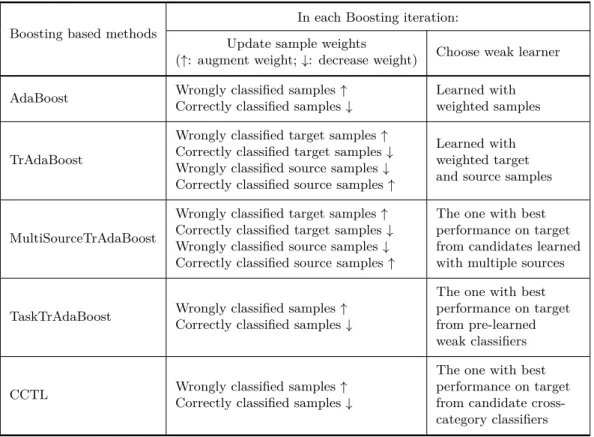
2.2.2 Boosting based methods . . . 53

2.2.3 Generative models . . . 57

2.3 Summary . . . 63

3 Discriminative Transfer Learning using Similarities and Dissimi-larities 67 3.1 Introduction. . . 67 3.2 Related work . . . 69 3.2.1 Transfer Learning . . . 69 3.2.2 Multi-task learning . . . 71 3.2.3 Sparse representation . . . 71

3.3 The proposed DTL algorithm . . . 73

3.3.1 Problem statement . . . 73

3.3.2 The Bi-SRC classifier . . . 74

3.3.3 The basic classification model . . . 77

3.3.4 Boosting the Area Under the ROC Curve . . . 80

3.4 Theoretical Analysis of the proposed DTL boosting. . . 83

3.4.1 Error bounds for DTL boosting . . . 84

3.4.2 Time complexity of DTL . . . 87

3.5 Experiments. . . 88

3.5.2 Results on the SUN dataset . . . 90

3.5.3 Analysis of the Experimental Results. . . 94

3.5.3.1 Effectiveness of the WMW statistic based cost func-tion . . . 95

3.5.3.2 Effectiveness of DTL in dealing with compact fea-ture vectors. . . 95

3.5.3.3 Effectiveness of using dissimilarities in addition to similarities . . . 96

3.6 Conclusion . . . 97

4 Optimal Transport for Deep Joint Transfer Learning 101 4.1 Introduction. . . 101

4.2 Related work . . . 103

4.3 Joint Transfer Learning Network . . . 104

4.3.1 Problem definition and the JTLN structure . . . 104

4.3.2 Optimal Transport Loss . . . 106

4.3.3 Back-propagation with OT Loss . . . 108

4.3.4 Choosing the cost metric . . . 110

4.3.4.1 MK-MMD as cost metric . . . 110

4.3.4.2 OT as cost metric . . . 112

4.4 Experiments. . . 112

4.4.1 Experiments on FGVC-Aircraft Dataset . . . 113

4.4.2 Experiments on Office-31 Dataset. . . 115

4.5 Conclusion and Future work . . . 116

5 Conclusion and Future Work 117

List of Tables

2.1 Boosting based transfer learning methods . . . 57

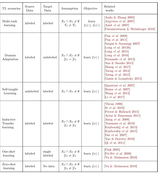
2.2 Some common transfer learning scenarios and their corresponding related works appeared in this chapter. The detailed explanation of the notations appeared in columns ‘Assumption’ and ‘Objective’ could be found in section 1.1.2. . . 64

3.1 Experimental results on the NUS-WIDE SCENE dataset (The re-sults are Average AUC (Area Under the ROC Curve) with standard deviation; the results in the first 5 rows are directly quoted from [Qi et al. 2011], the result for SparseTL is quoted from [Lu et al. 2014]) 90

3.2 Experimental results on the SUN dataset (Results in the first sub-table use 500-dimensional BOW features, while results in the second subtable use 50-dimensional AlexNet fc7 layer outputs as features. The experiments are carried out on a server with 100G memory and 4x8-cored AMD OpteronTM CPU 6128 @2GHz. The time unit is the second) . . . 94

3.3 Comparison of the WMW (Wilcoxon-Mann-Whitney) statistic based cost function with the MSE (Mean Squared Error) cost function used as selection criteria for dictionary pairs . . . 96

3.4 Benefits of using both positive and negative dictionaries. The Table on the left shows the results using average AUC as the performance metric, while the Table on the right shows the results using mean AP as the performance metric. In both Tables, the ‘Pos’ columns show DTL performance when using only positive dictionaries, while the ‘Pos+Neg’ columns show DTL performance when using both positive and negative dictionaries. The experiments are conducted on the SUN dataset. . . 97

4.2 Experimental Results on the ITL Datasets (results are multi-class classification accuracy) . . . 114

4.3 Experimental results on Office-31 Dataset: the number in brackets after each source domain is the number of images in this domain, the number pair in brackets after each target domain contains the number of training images and number of test images in this domain, the last two columns show accuracy results. . . 115

List of Figures

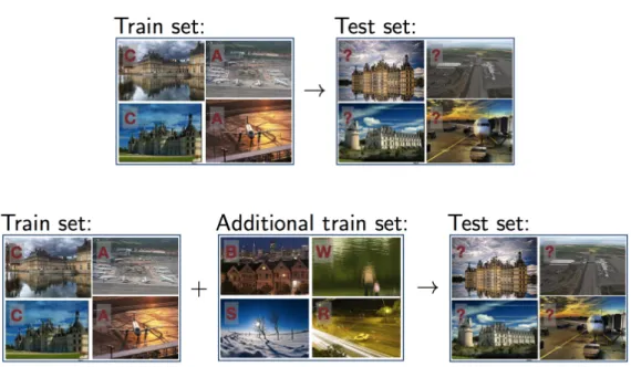
1.1 Comparison of traditional machine learning setting with transfer learning setting: in traditional machine learning setting, training set and test set should be formed with images from same categories and follow the same probability distribution; while in transfer learning setting, an additional training set is also given, which is allowed to have images from different data distribution, or even from different kind of categories. (The labels ‘C’ stands for ‘Castle’, ‘A’ stands for ‘Airport’, ‘B’ stands for ‘Building’, ‘W’ stands for ‘Water’, ‘S’ stands for ‘Snow’, ‘R’ stands for ‘Road’ and ‘?’ stands for unknown.) . . . . 5

2.1 Figure from [Parameswaran & Weinberger 2010]: An illustration of mt-lmnn(Multi task large margin nearest neighbors). The matrix

M₀ captures the communality between the several tasks, whereas

Mt for t > 0 adds the task specific distance transformation. . . . 33

2.2 Figure from [Long et al. 2015]: The DAN architecture for learning transferable features. Since deep features eventually transition from general to specific along the network, (1) the features extracted by convolutional layers conv1 – conv3 are general, hence these layers are frozen, (2) the features extracted by layers conv4 – conv5 are slightly less transferable, hence these layers are learned via fine-tuning, and (3) fully connected layers fc6 – fc8 are tailored to fit specific tasks, hence they are not transferable and should be adapted with MK-MMD. 37

2.3 Figure from [Ganin & Lempitsky 2015]: The proposed architecture includes a deep feature extractor (green) and a deep label predictor (blue), which together form a standard feed-forward architecture. Unsupervised domain adaptation is achieved by adding a domain classifier (red) connected to the feature extractor via a gradient re-versal layer that multiplies the gradient by a certain negative con-stant during the back-propagation-based training. Otherwise, the training proceeds in a standard way and minimizes the label predic-tion loss (for source examples) and the domain classificapredic-tion loss (for all samples). Gradient reversal ensures that the feature distributions over the two domains are made similar (as indistinguishable as possi-ble for the domain classifier), thus resulting in the domain-invariant features. . . 40

3.1 Nus-Wide Scene image dataset. In this Figure each bar represents a category: the height of the bar represents the number of positive samples in the corresponding category; the text on the top of each bar shows the category name and the number of positive samples; the first 10 categories with the fewest image samples are chosen as target categories, and the remaining 23 categories are treated as source categories . . . 89

3.2 SUN dataset: in this Figure each bar represents a category: the height of the bar represents the number of positive samples in the corresponding category; the text on the top of each bar shows the category name and the number of positive samples; the first 10 cate-gories with the fewest image samples are chosen as target catecate-gories, and the remaining 42 categories are treated as source categories. . . 91

3.3 Illustration of selected dictionary pairs for each classification model on the SUN dataset with BOW features. In each subfigure, the name of the target category is displayed on the top space of the Figure: the horizontal axis shows the number of dictionary pairs, and the vertical axis the weight for each dictionary pair; the chosen dictionary pairs are presented in the descending order of their weights, while above or in the bars are the names of the selected source categories which form the dictionaries: (+) stands for positive dictionary and (-) stands for negative dictionary. . . 99

3.4 Comparison of DTL with other methods on compact features. The graph on the left shows the result using average AUC as the perfor-mance metric, while the graph on the right shows the result using mean AP as the performance metric. In both graphs, the horizontal axis shows 3 different features: AN5D a set of 5-dimensional fea-tures, AN10D a set of 10-dimensional features and AN50D a set of 50-dimensional features. The experiments are conducted on the SUN dataset. . . 100

4.1 The structure and data flow of a Joint Transfer Learning Network based on Alexnet . . . 106

Abstract

When learning a classification model for a new target domain with only a small amount of training samples, brute force application of machine learning algorithms generally leads to over-fitted classifiers with poor generalization skills. On the other hand, collecting a sufficient number of manually labeled training samples may prove very expensive. Transfer Learning methods aim to solve this kind of problems by transferring knowledge from related source domain which has much more data to help classification in the target domain. Depending on different assumptions about target domain and source domain, transfer learning can be further categorized into three categories: Inductive Transfer Learning, Transductive Transfer Learning (Domain Adaptation) and Unsupervised Transfer Learning. We focus on the first one which assumes that the target task and source task are different but related. More specifically, we assume that both target task and source task are classification tasks, while the target categories and source categories are different but related. We propose two different methods to approach this ITL problem.

In the first work we propose a new discriminative transfer learning method, namely DTL, combining a series of hypotheses made by both the model learned with target training samples, and the additional models learned with source cate-gory samples. Specifically, we use the sparse reconstruction residual as a basic dis-criminant, and enhance its discriminative power by comparing two residuals from a positive and a negative dictionary. On this basis, we make use of similarities and dis-similarities by choosing both positively correlated and negatively correlated source categories to form additional dictionaries. A new Wilcoxon-Mann-Whitney statistic based cost function is proposed to choose the additional dictionaries with unbal-anced training data. Also, two parallel boosting processes are applied to both the positive and negative data distributions to further improve classifier performance. On two different image classification databases, the proposed DTL consistently

out-performs other state-of-the-art transfer learning methods, while at the same time maintaining very efficient runtime.

In the second work we combine the power of Optimal Transport and Deep Neu-ral Networks to tackle the ITL problem. Specifically, we propose a novel method to jointly fine-tune a Deep Neural Network with source data and target data. By adding an Optimal Transport loss (OT loss) between source and target classifier predictions as a constraint on the source classifier, the proposed Joint Transfer Learning Network (JTLN) can effectively learn useful knowledge for target classi-fication from source data. Furthermore, by using different kind of metric as cost matrix for the OT loss, JTLN can incorporate different prior knowledge about the relatedness between target categories and source categories. We carried out experi-ments with JTLN based on Alexnet on image classification datasets and the results verify the effectiveness of the proposed JTLN in comparison with standard con-secutive fine-tuning. To the best of our knowledge, the proposed JTLN is the first work to tackle ITL with Deep Neural Networks while incorporating prior knowledge on relatedness between target and source categories. This Joint Transfer Learning with OT loss is general and can also be applied to other kind of Neural Networks.

Keywords: Inductive Transfer Learning, Sparse Representation, Optimal Trans-port, Computer Vision.

Résumé

Lors de l’apprentissage d’un modèle de classification pour un nouveau domaine cible avec seulement une petite quantité d’échantillons de formation, l’application des algorithmes d’apprentissage automatiques conduit généralement à des classi-fieurs surdimensionnés avec de mauvaises compétences de généralisation. D’autre part, recueillir un nombre suffisant d’échantillons de formation étiquetés manuelle-ment peut s’avérer très coûteux. Les méthodes de transfert d’apprentissage visent à résoudre ce type de problèmes en transférant des connaissances provenant d’un domain source associé qui contient beaucoup plus de données pour faciliter la clas-sification dans le domaine cible. Selon les différentes hypothèses sur le domaine cible et le domaine source, l’apprentissage par transfert peut être classé en trois catégories: appentissage par transfert inductif, apprentissage par transfert trans-ducteur (adaptation du domaine) et apprentissage par transfert non surveillé. Nous nous concentrons sur le premier qui suppose que la tâche cible et la tâche source sont différentes mais liées. Plus pécisément, nous supposons que la tâche cible et la tâche source sont des tâches de classification, tandis que les catégories cible et les catégories source sont différentes mais liées. Nous proposont deux méthodes différentes pour aborder ce problème.

Dans le premier travail, nous proposons une nouvelle méthode d’apprentissage par transfert discriminatif, à savoir DTL(Discriminative Transfer Learning), com-binant une série d’hypothèses faites à la fois par le modèle appris avec les échantil-lons de cible et les modèles supplémentaires appris avec des échantiléchantil-lons des caté-gories sources. Plus précisément, nous utilisons le résidu de reconstruction creuse comme discriminant de base et améliore son pouvoir discriminatif en comparant deux résidus d’un dictionnaire positif et d’un dictionnaire négatif. Sur cette base, nous utilisons des similitudes et des dissemblances en choisissant des catégories sources positivement corrélées et négativement corrélées pour former des

dictio-nnaires supplémentaires. Une nouvelle fonction de coût basée sur la statistique de Wilcoxon-Mann-Whitney est proposée pour choisir les dictionnaires supplémen-taires avec des données non équilibrées. En outre, deux processus de Boosting parallèles sont appliqués à la fois aux distributions de données positives et néga-tives pour améliorer encore les performances du classificateur. Sur deux bases de données de classification d’images différentes, la DTL proposée surpasse de manière constante les autres méthodes de l’état de l’art du transfert de connaissances, tout en maintenant un temps d’exécution très efficace.

Dans le deuxième travail, nous combinons le pouvoir du transport optimal (OT) et des réseaux de neurones profond (DNN) pour résoudre le problème ITL. Plus précisément, nous proposons une nouvelle méthode pour affiner conjointement un réseau de neurones avec des données source et des données cibles. En ajoutant une fonction de perte du transfert optimal (OT loss) entre les prédictions du classifica-teur source et cible comme une contrainte sur le classificaclassifica-teur source, le réseau JTLN (Joint Transfer Learning Network) proposé peut effectivement apprendre des con-naissances utiles pour la classification cible à partir des données source. En outre, en utilisant différents métriques comme matrice de coût pour la fonction de perte du transfert optimal, JTLN peut intégrer différentes connaissances antérieures sur la relation entre les catégories cibles et les catégories sources. Nous avons effec-tué des expérimentations avec JTLN basées sur Alexnet sur les jeux de données de classification d’image et les résultats vérifient l’efficacité du JTLN proposé. A notre connaissances, ce JTLN proposé est le premier travail à aborder ITL avec des réseaux de neurones profond (DNN) tout en intégrant des connaissances antérieures sur la relation entre les catégories cible et source.

Mots clés: Inductive Transfer Learning, Sparse Representation, Optimal Trans-port, Computer Vision.

Introduction

Making machines that can learn and solve problems as humans is one of the most exciting and even controversial dreams of mankind. The corresponding research topic is called Artificial Intelligence (AI) and is defined as the study of “Intelligent agents”: any device that perceives its environment and takes actions that maxi-mize its chance of success at some goal [Russell et al. 1995]. Among many of the sub-topics of AI, one important research direction, which is commonly known as Machine Learning (ML), is to study the construction of algorithms that can learn from and make predictions on data. Arthur Samuel firstly defined Machine Learning as “the field of study that gives computers the ability to learn without being explic-itly programmed” [Samuel 1959]. The earliest theoretical foundations of Machine Learning are built by Valiant, who introduced the framework of Probably Approx-imately Correct (PAC) learning [Valiant 1984], and Vapnik, who casts the problem of ‘learning’ as an optimization problem [Vapnik & Vapnik 1998]. Nowadays ma-chine learning is a combination of several disciplines such as statistics, information theory, measure theory and functional analysis.

Depending on the nature of the learning “signal” or “feedback” available to a learning system, Machine Learning tasks are typically classified into three broad categories: Supervised Learning (where the computer is presented with example inputs and their desired outputs, the goal is to learn a general rule that maps inputs to outputs), Unsupervised Learning (where only example inputs are given without corresponding outputs, the goal is to find structure in the given inputs) and Reinforcement Learning (where the computer program interacts with a dynamic environment in which it must perform a certain goal, the program is provided feedback in terms of rewards and punishments as it navigates its problem space).

Depending on the desired output of a learning system, Machine Learning tasks can be categorized differently: in classification, inputs are divided into two or more classes, and the learner must produce a model that assigns unseen inputs to one or more of these classes; in regression, the outputs are continuous rather than discrete; in clustering, a set of inputs is to be divided into groups; in density estimation, the program finds the distribution of inputs in some space; and dimensionality reduction simplifies inputs by mapping them into a lower-dimensional space, etc.

Nowadays, technology is in constant evolution and the amount of data is every-day dramatically increasing. In particular, we are witnessing a spectacular growth in image and video data due to the rapid spread of electronic devices capable of recording and sharing pictures and videos (e.g. smart-phones, tablets, digital cam-eras, surveillance video recorders, etc.) all around the world. Consequently, billions of raw images and videos are diffused on the Internet. For instance, 612 million of pictures are uploaded on Flickr during the year 20161_{, and approximately 400}

hours of new videos are uploaded on Youtube every minute according to a recent report in 20172. However, most of these images and video content are difficult to exploit because they have not been properly labeled or edited. Therefore, automatic classification of images becomes a quite urgent need. In this thesis, we mainly focus on the supervised classification of images.

Ideally, when enough labeled training samples are given, the supervised clas-sification problem could be formalized as an Empirical Risk Minimization (ERM) problem where we search in the hypothesis space for a hypothesis that can minimize the empirical risk on training samples. Thanks to Hoeffding’s inequality, when the hypothesis space is properly chosen and the training set is large enough, the learned hypothesis could have a bounded generalization error (i.e., the difference between

the empirical risk and the expected risk) which guarantees its good performance on

same distributed test samples.

However, in reality this is not always the case. A common problem is that collecting a sufficient number of manually labeled training samples is very

expen-1_{https://www.flickr.com/photos/franckmichel/6855169886} 2_{https://expandedramblings.com/index.php/youtube-statistics/}

sive. Especially with the rapid increase of Web data, most of the Web collected images are unlabeled or with very noisy labels. When the number of images is enormous, manually labelling them would be expensive and time-consuming. Fur-thermore, when dealing with visual data, a frequently encountered problem is that even for a same semantic concept, the images obtained can be surprisingly different by using different sensors, under different lighting conditions, or having different backgrounds, etc.. These kind of problems give birth to a pressing need for algo-rithms that can learn efficiently from a small amount of labeled training data by leveraging knowledge from related unlabeled or noisy labeled data or differently distributed data. The research direction that deals with these kind of problems is called ‘Transfer Learning’.

The study of Transfer Learning is motivated by the fact that human, even a child, can intelligently apply knowledge learned previously to solve new problems efficiently. An example in [Quattoni et al. 2009] gives an evidence on this point: when a child learns to recognize a new letter of the alphabet he will use examples provided by people with different hand-writing styles using pens of different colors and thicknesses. Without any prior knowledge a child would need to consider a large set of features as potentially relevant for learning the new concept, so we would expect the child to need a large number of examples. But if the child has previously learnt to recognize other letters, he can probably discern the relevant attributes (e.g. number of lines, line curvatures) from irrelevant ones (e.g. the color of the lines) and learn the new concept with a few examples. The fundamental motivation for Transfer Learning in the field of Machine Learning was discussed in a NIPS-95 workshop on “Learning to Learn”, which focused on the need for lifelong machine learning methods that retain and reuse knowledge which are learned previously. Research on Transfer Learning has attracted more and more attention since 1995. Compared to traditional machine learning techniques which try to learn each task from scratch, transfer learning techniques try to transfer the knowledge from some previous tasks to a target task when the latter has fewer high-quality training data. The goal of this thesis is to develop efficient transfer learning algo-rithms for images classification. In the following we will firstly give a formal

description of this problem, and then introduce our contributions.

1.1

Problem definition

1.1.1 Image classification

In an image classification task our goal is to learn a mapping from images to class labels. The input images could be represented by pre-extracted feature vectors (as in chapter 3) or image pixels directly (as in chapter 4), we can therefore assume a vector x ∈ Rd _{as notation for an image, with d the number of feature dimensions}

or number of pixels. For the output class labels, we can either consider binary classification (as in chapter3) or multi-class classification (as in chapter4). In both cases we can either represent the label of an image with a scalar y (y _{∈ {+1, −1} for} binary classification or y a discrete value as class index for multi-class classification) or a vector y_{∈ {0, 1}}n_{, with n the number of classes.}

To build an efficient image classification model, there are two key problems that need to be solved. The first one is to find a discriminative feature space in which the class distributions can be easily distinguished from each other, this can either be done by feature selection (i.e., selecting most discriminative features), or by mapping the samples into a new feature space (e.g., traditional feature extraction techniques such as SIFT (Scale-Invariant Feature Transform) or HOG (Histogram of Oriented Gradient), or the recent representation learning techniques such as Dictionary Learning or Convolutional Neural Networks (CNNs)). The second one is to build a proper classifier which maps samples from the feature space to the class label space. The classifier can either be a generative model which learns the joint distribution p(x, y) (e.g.,mixture models) or a discriminative model which learns the conditional distribution p(y_{|x) (e.g., Support Vector Machines (SVMs)).}

In the computer vision community, the first problem is usually the most con-cerned one, especially with the rapid evolution of Deep Neural Networks, a good feature representation learned with Convolutional Neural Networks can give excel-lent classification performance even with a simple classifier (e.g., softmax classifier or K-Nearest Neighbors classifier). However, the second problem is also important,

especially for transfer learning problems in which we only have a few target train-ing samples. Dependtrain-ing on the techniques used, these two problems can sometimes be treated in a unified model (e.g., in CNNs the feature extraction layers and the softmax classifier are integrated in a unified Deep Neural Network).

1.1.2 Transfer Learning

Figure 1.1: Comparison of traditional machine learning setting with transfer learn-ing settlearn-ing: in traditional machine learnlearn-ing settlearn-ing, trainlearn-ing set and test set should be formed with images from same categories and follow the same probability dis-tribution; while in transfer learning setting, an additional training set is also given, which is allowed to have images from different data distribution, or even from differ-ent kind of categories. (The labels ‘C’ stands for ‘Castle’, ‘A’ stands for ‘Airport’, ‘B’ stands for ‘Building’, ‘W’ stands for ‘Water’, ‘S’ stands for ‘Snow’, ‘R’ stands for ‘Road’ and ‘?’ stands for unknown.)

In this section, we follow the notations introduced in [Pan & Yang 2010a] to describe the problem statement of transfer learning. A domain _{D consists of two} components: a feature space_{X and a marginal probability distribution P (x), where}

x_{∈ X . In general, if two domains are different, then they may have different feature}

spaces or different marginal probability distributions. Given a specific domain,

D = {X , P (x)}, a task T consists of two components: a label space Y and a

function (i.e., a mapping from the feature space to the label space) that can be used to make predictions on unseen instances. From a probabilistic viewpoint, f (x) can also be written as the conditional distribution P (y_|x).

Based on the notations defined above, the definition of transfer learning can be defined as follows [Pan & Yang 2010a],

Definition 1. Given a source domain _DS and learning task TS, a target domain

DT and learning task TT, transfer learning aims to help improve the learning of

the target predictive function fT(·) in DT using the knowledge inDS andTS, where

DS ̸= DT, or TS ̸= TT.

In the above definition, a domain is a pair _{D = {X , P (x)}, thus the condition}

DS ̸= DT implies that either XS ̸= XT or P (xS) ̸= P (xT). Similarly, a task is

defined as a pair T = {Y, P (y|x)}, thus the condition TS ̸= TT implies that either

YS ̸= YT or P (yS|xS) ̸= P (yT|xT). When the target and the source domains are

the same, i.e. DS =DT, and their learning tasks are the same, i.e. TS =TT, the

learning problem becomes a traditional machine learning problem. An illustration which compares the traditional machine learning setting and the transfer learning setting is given in Figure 1.1.

Based on different conditions for differences between source domain and tar-get domain and differences between source task and tartar-get task, transfer learning scenarios can be categorized differently. For example, based on whether the fea-ture spaces or label spaces are identical or not, transfer learning is categorized into two settings [Pan 2014]: 1) homogeneous transfer learning (where the inter-section between source and target feature spaces is not empty (XS∩ XT ̸= ∅) and

source and target label spaces are the same (_YS = YT), while source and target

marginal distributions and conditional distributions are different (P (xS) ̸= P (xT)

or P (y_S|xS) ̸= P (yT|xT))), and 2) heterogeneous transfer learning (where the

two feature spaces have empty intersection or the two label spaces are different

(_{XS∩ XT} =∅ or YS̸= YT)).

Another way to categorize transfer learning is based on whether the two domains or two tasks are identical or not [Pan & Yang 2010a], we have: 1) inductive transfer

learning (where source and target domains are the same, while source and target

tasks are different but related), 2) unsupervised transfer learning (where source and target domains are different but related, and source and target tasks are also different but related), and 3) transductive transfer learning (where source and target domains are different but related, while source and target tasks are the same).

In this thesis, we mainly focus on the transfer learning scenario where the in-tersection between source and target feature spaces is not empty (_XS ∩ XT ̸= ∅)

while the source and target label spaces are different (_{YS ̸= YT}). According to the two categorization methods shown above, this scenario can be categorized as

heterogeneous transfer learning or inductive transfer learning.

Specifically, in chapter 3 we consider binary classification problem. We assume having a target domain _DT with a binary classification task _TT, which can be accessed through a small set of target training data. We also assume having a source domain _DS with multiple source binary classification tasks _TS,1, . . . ,TS,L,

which can be accessed through a large set of source training data. As mentioned in the previous paragraph, here_{XS∩ XT ̸= ∅ and YS,i̸= YT},_{∀i ∈ [1, L]. The aim is to} learn a discriminative predictive function for the target task using both the target training data and the source training data.

In chapter 4 we consider multi-class classification problem. We assume having a target domain _DT with a multi-class classification task _TT, along with a source domainDSwith a multi-class classification taskTS. Similarly we assumeXS∩XT ̸=

∅ and YS ̸= YT. The aim is also to learn a discriminative predictive function for

the target task using both the target training data and the source training data.

1.2

Thesis Contributions

As mentioned above, in this thesis we study the heterogeneous inductive transfer

learning scenario for image classification. Specifically, we propose two different

approaches to tackle this problem:

• In chapter 3 we propose a novel discriminative knowledge transfer method, which leverages relatedness of various source categories with the target

cate-gory to enhance learning of the target classifier. The proposed Discriminative Transfer Learning (DTL) explicitly makes use of both positively and nega-tively correlated source categories to help classification of the target category. Specifically, DTL chooses from source categories the most positively and neg-atively correlated categories to act as positive and negative dictionaries for discriminative classification of target samples using reconstruction residuals on these dictionaries. We further enhance the performance of DTL by con-currently running two AdaBoost processes on the positive and negative distri-butions of the target training set. A novel Wilcoxon-Mann-Whitney(WMW)-based cost function is also introduced in DTL to deal with the unbalanced nature of data distribution.

The main contributions of this work are fourfold:

1. We highlight the importance of learning both similarity and dissimilarity in a transfer learning algorithm through joint use of positively correlated and negatively correlated source categories, and introduce a Bi-SRC clas-sifier as the building block of the proposed DTL.

2. We propose a novel cost function based on the Wilcoxon-Mann-Whitney (WMW) statistic, and apply two parallel boosting processes, both on positive data and on negative data distribution, thus successfully avoid-ing the effect of unbalanced data distribution.

3. We conduct theoretical analyses on the proposed DTL algorithm and provide theoretical guarantees both in terms of error bound and time complexity.

4. Using different features and evaluating on two different performance met-rics, we benchmark the proposed DTL on two different databases for the task of image categorization. We also consistently demonstrate the ef-fectiveness of the proposed DTL: it displays the best performance with a large margin in comparison to several state-of-the-art TL methods, with a runtime that can prove 80 times faster in training and 66 times faster in testing than the other state-of-the-art TL methods that it has been

compared with.

• In chapter 4 we propose a novel method to jointly fine-tune a Deep Neu-ral Network with both source data and target data. In contrast to naive joint fine-tuning, we propose to explicitly account for the relatedness between source and target tasks and explore such prior knowledge through the design of a novel loss function, namely Optimal Transport loss (OT loss), which is minimized during joint training of the underlying neural network, in order to bridge the gap between the source and target classifiers. This results in a Joint Transfer Learning Network (JTLN) which can be built upon common Deep Neural Network structure. In JTLN, the source data and target data go through same feature extraction layers simultaneously, and then separate into two different classification layers. The Optimal Transport loss is added between the two classification layers’ outputs, in order to minimize the dis-tance between two classifiers’ predictions. As the Optimal Transport loss is calculated with a pre-defined cost matrix, this JTLN can therefore incorpo-rate different prior knowledge about the relations between source and target tasks by using different kind of cost metric. We show two examples of using the distances between category distributions as cost metric.

The contributions of this work are threefold:

1. We propose a Joint Transfer Learning framework built upon existing Deep Neural Networks for Inductive Transfer Learning.

2. We extend the Wasserstein loss proposed in [Frogner et al. 2015] to a more general Optimal Transport loss for comparing probability measures with different length, and use it as a soft penalty in our JTLN.

3. We show two different ways of using the distance between category dis-tributions as cost metric for OT loss. Experimental results on two ITL image classification datasets show that JTLN with these two cost metrics can achieve better performance than consecutive fine-tuning or simple joint fine-tuning without extra constraint.

1.3

Outline of the thesis

The structure of this thesis is as follows: chapter 2 reviews existing related work on general transfer learning algorithms and transfer learning algorithms for vi-sion recognition problems; chapter 3describes in detail our work on Discriminative Transfer Learning using both similarities and dissimilarities; chapter4 describes in detail our work on Joint Transfer Learning Network. Finally, in chapter 5we draw conclusions and discuss future lines of research.

Literature Review

In this chapter we review related works on general transfer learning algorithms as well as previous literature on transfer learning algorithms for vision recognition problems.

Following the two main problems for image classification (which are also the key problems for vision recognition tasks) introduced in section 1.1.1, we can ap-proximately categorize related transfer learning algorithms into two categories: 1) feature representation level knowledge transfer; and 2) classifier level knowledge transfer. We will introduce these two categories in detail in the following sections.

2.1

Feature representation level knowledge transfer

Feature representation level knowledge transfer algorithms mainly focus on learn-ing a feature representation which is discriminative for target task by leveraglearn-ing knowledge from both target training data and source data. Normally these methods assume that there exists a mapping from the original input space to an underlying shared feature representation. This latent representation captures the information necessary for training classifiers for source and target tasks. The goal of these algorithms is therefore to uncover the underlying shared representation and the parameters of the classifier for target task.

Grouped by the feature mapping techniques used by different algorithms, we will mainly introduce five lines of research works in this section:

In section 2.1.1 we introduce some early transfer learning algorithms which learns a shared representation with shallow Neural Networks or linear transforma-tions. Most of these works are proposed for the multi-task learning scenario, which

considers source tasks and target tasks equally and aim to share knowledge across all related tasks.

In section 2.1.2 we introduce some transfer learning algorithms which learns a shared representation using conventional dimensionality reduction methods. Most of these works are proposed for the domain adaption scenario, which is also a sub-topic of transfer learning and aim at adapting distributions between source data and target data.

In section 2.1.3 we introduce some transfer learning algorithms which learn underlying feature space through the metric learning framework.

In section 2.1.4 we introduce some recent transfer learning algorithms which make use of the Deep Neural Networks as feature mapping. Similar to the methods in section 2.1.2, these algorithms are also proposed for domain adaptation scenar-ios. Since nowadays deep neural networks are the state-of-the-art feature learning architecture, these DNN based transfer learning algorithms are also the current state-of-the-art methods for domain adaptation.

In section2.1.5we introduce some knowledge transfer algorithms based on dic-tionary learning (also known as sparse coding) which are designed for the self-taught

learning scenario. Since in self-taught learning we perform knowledge transfer from

unlabeled source samples which are easy to collect, this is a hard but promising sub-problem of transfer learning.

2.1.1 Representation Learning with Shallow Neural Networks and linear transformations

2.1.1.1 Transfer learning with shallow Neural Networks

One of the earliest works on transfer learning was [Thrun 1996] which introduced the concept of lifelong learning. Thrun proposed a transfer algorithm that uses source training data to learn a function, denoted by g : I _{→ I}′, which maps input samples in feature space I to a new feature space I′. The main idea is to find a new representation where every pair of positive examples for a task will lie close to each other while every pair of positive and negative examples will lie far from each

other.

LetPkbe the set of positive samples for the k-th task andNkthe set of negative

samples, Thrun’s transfer algorithm minimizes the following objective:

min g∈G m ∑ k=1 ∑ xi∈Pk ( ∑ xj∈Pk ∥ g(xi)− g(xj)∥ − ∑ xj∈Nk ∥ g(xi)− g(xj)∥ ) (2.1)

where _{G is the set of transformations encoded by a two layer neural network.} The transformation g(·) learned from the source data is then used to project the samples of the target task into the new feature space. Classification for the target task is performed by running a nearest neighbor classifier in the new space.

The paper presented experiments on a small object recognition task. The results showed that when labeled data for the target task is scarce, the representation obtained by running their transfer algorithms on source training data could improve the classification performance of a target task.

This work is further generalized by several authors [Ando & Zhang 2005] [Argyriou et al. 2007] [Amit et al. 2007]. The three works can all be casted under the framework of ‘structural learning’ proposed in [Ando & Zhang 2005].

2.1.1.2 Structural learning methods

In a structural learning framework we assume the existence of task-specific pa-rameters wk for each task and shared parameters θ that parameterize a family of

underlying transformations. Both the structural parameters and the task-specific parameters are learned together via joint risk minimization on some supervised training data for m related tasks.

Consider learning linear predictors of the form h_k(x) = wT_kv(x) for some w∈ Rz

and some transformation v ∈ V : Rd _{→ R}z_{. In particular, let V be the family of}

linear transformations: vθ_{(x) = θx where θ is a z by d matrix that maps a d}

dimensional input vector to a z dimensional space.

Define the task-specific parameters matrix: W = [w₁, . . . , wm] where wk∈ Rz

hidden feature and the k-th task. A structural learning algorithm finds the optimal task-specific parameters W∗ and structural parameters θ∗ by minimizing a jointly regularized empirical risk:

arg min W,θ m ∑ k=1 1 nk nk ∑ i=1 Loss(w⊤_kθxk_i, yk_i) + γΦ(W ) + λΨ(θ) (2.2)

The first term in equation (2.2) measures the mean error of the m classifiers by means of some loss function Loss(_{·). The second term is a regularization penalty} on the task-specific parameters W and the last term is a regularization penalty on the structural parameters θ. Different choices of regularization functions Φ(W ) and Ψ(θ) result in different structural learning algorithms.

[Ando & Zhang 2005] combine a l₂ regularization penalty on the task-specific parameters with an orthonormal constraint on the structural parameters, resulting in the following objective:

arg min W,θ m ∑ k=1 1 nk nk ∑ i=1 Loss(w⊤_kθxk_i, y_ik) + γ m ∑ k=1 ∥ wk∥22, s.t. θθT = I (2.3)

where θ is a z by d matrix, z is assumed to be smaller than d and its optimal value is found using a validation set. Therefore knowledge transfer is realized by mapping the high dimensional feature vector x to a new feature vector θ_{· x in a} shared low dimensional feature space. The authors propose to solve (2.3) using an alternating minimization procedure. This algorithm is applied in the context of asymmetric transfer where auxiliary (i.e. source) training sets are utilized to learn the structural parameter θ. The learned structural parameter is then used to project the samples of the target task and train a classifier on the new feature space. The paper presented experiments on text categorization where the source training sets were automatically derived from unlabeled data (this algorithm can therefore be regarded as a semi-supervised training algorithm). their results showed that the proposed algorithm gave significant improvements over a baseline method that trained on the labeled data ignoring the source training sets.

This work is further applied to image classification in [Quattoni et al. 2007] in which they consider having a large set of images with associated captions, while among them only a few images are annotated with story news labels. They take the prediction of content words from the captions to be the source tasks and the prediction of a story label to be the target tasks. The goal is to leverage the source tasks to derive a lower dimensional representation that captures the rele-vant information necessary to discriminate between different stories. They perform experiments with this method both on synthetic data and real news image data. Results show that when source data labels are suitably related to a target task, the structural learning method can discover feature groupings that speed up learning of the target task.

[Argyriou et al. 2007] proposed an alternative model to learn shared represen-tations. In their approach the structural parameter θ is assumed to be a d by d matrix, i.e. the linear transformation does not map the inputs x to a lower di-mensional space. Instead, sharing of hidden features across tasks is realized by a regularization penalty imposed on the task-specific parameters W , which requires only a few hidden features to be used by any task (i.e. requires the matrix W to be row-sparse). This regularization is achieved by using the following matrix norm:

l1,2(W ) =

∑z

j=1 ∥ wj ∥2, which is known to promote row sparsity in W . Therefore

the objective can be written as:

arg min W,θ m ∑ k=1 1 nk nk ∑ i=1 Loss(w⊤_kθxk_i, y_ik) + γl1,2(W ) (2.4)

The authors showed that this problem is equivalent to a convex problem for which they developed an alternating minimization algorithm. The paper presented experiments on a product rating problem where the goal is to predict ratings given by different subjects. In the context of multi-task learning predicting the ratings for a single subject can be regarded as a task. The transfer learning assumption is that predictions made by different subjects are related. The results showed that their algorithm gave better performance than a baseline model where each task was trained independently with an l1 penalty.

[Amit et al. 2007] proposed a regularization scheme for transfer learning based on a trace norm regularization penalty. Consider the following m by d parameter matrix W = [w1_{, w}2_{, . . . , w}m_{], where each row corresponds to the parameters of one}

task. The transfer algorithm minimizes the following jointly regularized objective:

arg min W m ∑ k=1 1 nk nk ∑ i=1 Loss(w⊤_kxk i, yik) + γΩ(W ) (2.5)

where Ω(W ) = ∑_{i|γi| and γi} is the i-th eigenvalue of W . This norm is used because it is known to induce low rank on solution matrices W [Srebro & Jaakkola 2003]. Recall that the rank of a d by m matrix W is the mini-mum z such that W can be factored as W = θ⊤W′, for a z by m matrix W′ and a

z by d matrix θ.

Notice that θ is no longer in equation (2.5), this is because in this formulation we do not search explicitly for a transformation θ. Instead, we utilize the regularization penalty Ω(W ) to encourage solutions where the task-specific parameters W can be expressed as the combination of a few basis shared across tasks. This optimiza-tion problem can be expressed as a semi-definite program and can be solved with an interior-point method. However, the authors argue that interior point methods scale poorly with the size of the training set and proposed a gradient based method to solve this problem by minimizing a smoothed approximation of (2.5). The au-thors conducted experiments on a multi-class classification task where the goal is to distinguish between 72 classes of mammals. The performance of their transfer learning algorithm is compared to that of a baseline multi-class SVM classifier. Their results show that the trace-norm penalty can improve multi-class accuracy when only a few samples are available for training.

2.1.2 Representation Learning with dimensionality reduction

methods

In the previous section 2.1.1, we have introduced some early works on representa-tion learning using shallow neural networks or linear transformarepresenta-tions. A common assumption of these works is that they assume a representation mapping learned

with the source data can be directly applied to target data. This is a strong as-sumption which requests the source data to be very close to the target data, if not the knowledge transfer with the learned representation mapping will fail.

In this section and the next section 2.1.4 we introduce some transfer learn-ing algorithms with distribution adaptation which relax this assumption and learn the shared representation by explicitly minimize predefined distance measures to reduce the differences between source and target in the marginal distribu-tion [Si et al. 2010] [Pan et al. 2008] [Pan et al. 2011], or in the conditional dis-tribution [Satpal & Sarawagi 2007], or both [Long et al. 2013b] [Long et al. 2015] [Long et al. 2016]. These works are mostly proposed for the Domain Adaptation scenario, which is a subproblem of transfer learning.

Recall the notations defined in section 1.1.2, assume having a target domain

DT = {XT, P (xT)} with a target task TT = {YT, P (yT|xT)} (here conditional

probability P (y_T|xT) is equivalent to the prediction function fT(·)), and a source

domain _DS = {XS, P (xS)} with a source task TS = {YS, P (yS|xS)}. Given the

assumptions: _XS =XT, YS =YT, P (xS)̸= P (xT) and P (yS|xS) ̸= P (yT|xT), the

transfer learning algorithms by distribution adaptation aim to learn a new feature representation in which the distribution differences between P (x_S) and P (xT), or

between P (yS|xS) and P (yT|xT), or both of them are explicitly reduced.

2.1.2.1 Adaptation with Bregman divergence based distance measure

In [Si et al. 2010] the authors proposed a Bregman Divergence based regularization schema for transfer subspace (representation) learning, which combines Bregman divergence with conventional dimensionality reduction algorithms. Similar to the

structural learning schema introduced in section 2.1.1, this regularized subspace

learning also learns a feature mapping and a classifier at the same time. The

difference between this work and the structural learning framework is that the reg-ularization term on the feature transformation parameters is based on a bregman

divergence between the source marginal distribution and the target marginal

dis-tribution. Therefore the difference between the two marginal distributions will be explicitly reduced during optimization.

Specifically, assume some feature transformation vθ_{(x) = θx where θ is a z by}

d matrix that maps the original d dimensional input feature vector into a new z

dimensional feature space. In subspace learning framework we learn this matrix θ by minimizing a specific objective function F (θ):

θ∗= arg min

θ∈Rz×d

F (θ) (2.6)

The objective function F (θ) is designed for specific applications, here it mini-mizes the data classification loss in the selected subspace according to different as-sumptions or intuitions. For example, Fisher’s linear discriminant analysis (FLDA) selects a subspace, where the trace ratio of the within-class scatter matrix and the between-class scatter matrix is minimized.

To reduce the distribution difference between source and target data, the au-thors propose a Bregman divergence based regularization term Dθ(PS ∥ PT) which

measure the distribution difference of samples drawn from different domains in the projected subspace θ. By integrating this regularization into (2.6), we obtain a new framework for transfer subspace learning (TSL):

θ∗= arg min

θ∈Rz×d

F (θ) + λDθ(PS∥ PT) (2.7)

with respect to specific constraints, e.g., θ⊤θ = I. Here λ is the regularization

parameter that controls the trade-off between the two terms in (2.7).

Let v : I _{→ I}′ be a C1 _{convex function defined on a closed convex set I ⊂}

R+_{. We denote the first order derivative of v by v}′_{, denote its inverse function}

by ξ = (v′)−1. The probability density for the source and target samples in the projected subspace I′ is PS(v(x)) and PT(v(x)) respectively. The regularization

term is defined as follows:

Dθ(PS ∥ PT) =

∫

d(ξ(PS(v(x))), ξ(PT(v(x))))dµ (2.8)

where d(ξ(P_S(v(x))), ξ(PT(v(x)))) is the difference at ξ(PT(v(x))) between the

du(v(x))) is the Lebesgue measure. The right hand side of (2.8) is also called the U-divergence on the subspaceRd_.

The authors show examples of this transfer subspace learning framework using different F (θ) (i.e. combining with different dimensionality reduction methods), such as transfered principal components analysis (TPCA), transfered Fisher’s linear discriminant analysis (TFLDA), transfered locality preserving projections (TLPP) with supervised setting, etc. They present experimental evidence on both face image data sets and text data sets, suggesting that the proposed framework is effective to deal with cross-domain learning problems.

2.1.2.2 Adaptation with Maximum Mean Discrepancy (MMD) as dis-tance measure

Similar to the previous approach, in [Pan et al. 2008] the authors proposed a trans-fer learning algorithm which also combines conventional dimensionality reduction method and a distance measure for measuring the distance between marginal dis-tributions of source data and target data. In this work the authors make use of the Maximum Mean Discrepancy as distribution distance measure, and PCA as the dimensionality reduction method.

Maximum Mean Discrepancy (MMD) is a two samples test criterion for com-paring distributions based on Reproducing Kernel Hilbert Space (RKHS). Let

X = {x1, . . . , xn1} and Y = {y1, . . . , yn2} be two random variable sets from

dis-tributions_{P and Q, respectively, and H be a universal RKHS with the reproducing} kernel mapping ϕ: f (x) =⟨ϕ(x), f⟩, ϕ : X → H. The empirical estimate of distance between_{P and Q defined by MMD is as follows:}

Dist(X, Y ) =∥ 1 n1 n1 ∑ i=1 ϕ(xi)− 1 n2 n2 ∑ i=1 ϕ(yi)∥H (2.9)

As can be seen, the MMD between two sample sets is equivalent to the distance between the means of the two sample sets mapped into a RKHS. Based on this, the authors proposed a new dimensionality reduction method, denoted as MMDE (Maximum Mean Discrepancy Embedding), to learn a low-dimensional latent space

F common to source and target domains. A classifier is then learned in this latent

space with source labeled data, and this learned classifier is directly used for tar-get classification task (i.e., they assume that in the latent space the conditional distributions of source data and target data are the same).

Denote the source domain data as Dsrc ={(xsrc1 , ysrc1 ), . . . , (xsrcn1, y

src

n1 )}, where

xsrc_i ∈ Rm is the input sample feature and ysrc

i the corresponding label. Similarly,

denote the target domain data as _Dtar ={(xtar₁ , ytar₁ ), . . . , (xtar_n2 , y_ntar₂ )} with xtar_i ∈ Rm_{. Let the feature projection map be ψ. Then learning a common low-dimensional}

latent space in which the distributions of the source and target data (i.e., X_src′ and

X_tar′ ) can be close to each other is equivalent to minimizing the MMD between X_src′ and X_tar′ :

Dist(X_src′ , X_tar′ ) = Dist(ψ(Xsrc), ψ(Xtar))

=∥ 1 n1 n1 ∑ i=1 ϕ◦ ψ(xsrc_i )− 1 n2 n2 ∑ i=1 ϕ◦ ψ(xtar_i )∥ (2.10)

Denote the corresponding kernel of ϕ◦ ψ by k, then equation (2.10) can be written in terms of the kernel matrices defined by k as:

Dist(X_src′ , X_tar′ ) = trace(KL) (2.11)

where K =  Ksrc,src Ksrc,tar Ktar,src Ktar,tar   ∈ R(n1+n2)×(n1+n2)

is a composite kernel matrix, and L = [Lij]⪰ 0 with

Lij =              1 n2 1 xi, xj ∈ Xsrc, 1 n2 2 xi, xj ∈ Xtar, − 1 n1n2 otherwise.

so we can learn this kernel matrix instead of learning the universal kernel k. Thus, the embedding problem can be formulated as the following optimization problem:

min K= eK+εI trace(KL)_{− λtrace(K)} s.t. Kii+ Kjj− 2Kij = d2ij, ∀(i, j) ∈ N , K1 = 0, eK ⪰ 0. (2.12)

where ε is a small positive constant and 1 and 0 are the vectors of ones and zeros, respectively. The second term is added to unfold the high dimensional data by maximizing the trace of K. This optimization problem can be further rewritten as a semidefinite program (SDP) which learns eK and can be solved by standard SDP

solvers. After obtaining eK, the authors then apply PCA and select the leading eigen

vectors to construct low-dimensional representations X_src′ and X_tar′ . A classifier is learned with X_src′ and Y_srcand is applied directly for classification in target domain. The authors perform experiments on indoor WiFi localization dataset and text classification dataset, the results showed that the proposed MMDE can effectively improve the performance compared to traditional machine learning algorithms.

2.1.2.3 Transfer Component Analysis

The previous MMDE suffers from two major limitations: (1) it is transductive, and does not generalize to out-of-sample patterns; (2) it learns the latent space by solv-ing a semi-definite program (SDP), which is a very expensive optimization problem. Furthermore, in order to construct low-dimensional representations, in MMDE the obtained K has to be further post-processed by PCA, this step may discard poten-tially useful information in K. To get ride of these limitations, the authors further proposed in [Pan et al. 2011] a new approach, named transfer component analysis (TCA), which tries to learn a set of common transfer components underlying both domains such that the difference in data distributions in the new subspace of two domains can be reduced, and data properties can be preserved.

gener-alized to out-of-sample patterns. Besides, instead of using a two-step approach, they propose a unified kernel learning method which utilizes an explicit low-rank representation.

First note that the kernel matrix K defined in (2.11) can be decomposed as K =

(KK−1/2)(K−1/2K), which is often known as the empirical kernel map. Consider

the use of a matrix fW ∈ R(n1+n2)×m that transforms the empirical kernel map

features to an m-dimensional space (where m _{≪ n}1+ n2). The resultant kernel

matrix is then

e

K = (KK−1/2fW )(fW⊤K−1/2K) = KW W⊤K (2.13)

where W = K−1/2fW . This kernel eK facilitates a readily parametric form for

out-of-sample kernel evaluations. On using the definition of eK in (2.13), the MMD distance between the two domains X_src′ and X_tar′ can be written as:

Dist(X_src′ , X_tar′ ) = trace((KW W⊤K)L) = trace(W⊤KLKW ) (2.14)

In minimizing (2.14), a regularization term trace(W⊤W ) is usually needed to

control the complexity of W . This regularization term can also avoid the rank deficiency of the denominator in the generalized eigenvalue decomposition.

Besides reducing the distance between the two marginal distributions, the pro-jection ϕ should also preserve data properties that are useful for the target super-vised learning task. As in PCA or KPCA, this can be done by preserving the data variance. Therefore by combining the minimization of distribution difference and preserving of the data variance, the kernel learning problem becomes:

min

W trace(W

⊤_{KLKW ) + µ trace(W}⊤_{W )}

s.t. W⊤KHKW = Im

(2.15)

pro-jected samples with H = In1+n2−(1/n1+ n2)11⊤ the centering matrix, 1∈ R

n1+n2

is the column vector with all 1’s, and In1+n2 ∈ R(n1+n2)×(n1+n2) Im ∈ Rm×m are

identity matrix. Though this optimization problem involves a non-convex norm constraint W⊤KHKW = Im, the authors proved that it can still be solved

effi-ciently by the following trace optimization problem:

max

W trace((W

⊤_{(KLK + µI}

m)W )−1W⊤KHKW ) (2.16)

Similar to kernel Fisher discriminant analysis [Muller et al. 2001], the W so-lutions in (2.16) are the m leading eigenvectors of (KLK + µI)−1KHK, where

m ⩽ n1 + n2− 1. This unsupervised approach is named TCA (Transfer

Compo-nent Analysis), based on this, the authors also proposed a semi-supervised version SSTCA. The effectiveness and efficiency of TCA and SSTCA are verified by exper-iments on five toy datasets and two real-world applications: cross-domain indoor WiFi localization and cross-domain text classification.

2.1.2.4 Joint Distribution Adaptation

The previous three works all focus on adapting the marginal distribution difference between source and target data, while assuming that the conditional distributions of source and target data in the learned new feature space are equal so that a classifier learned on source data can be directly applied to target data. However in reality the equality assumption of conditional distributions is strong and cannot always be respected. In [Long et al. 2013b] the authors proposed a transfer learning approach, referred to as Joint Distribution Adaptation (JDA), which aims to jointly adapt both the marginal distribution and conditional distribution in a principled dimensionality reduction procedure. Similar to MMDE and TCA, which are introduced previously, JDA also make use of Maximum Mean Discrepancy as the distance measure between distributions.

Assume (xs, ys) represent a labeled sample from source training set, xt

repre-sent an unlabeled sample from target training set, P (x_s) and P (xt) represent the