Classical Losses in Soft Magnetic Composites using Homogenization Techniques

HAL Id: tel-01576559

https://tel.archives-ouvertes.fr/tel-01576559

HAL is a multi-disciplinary open access archive for the deposit and dissemination of sci-entific research documents, whether they are pub-lished or not. The documents may come from teaching and research institutions in France or abroad, or from public or private research centers.

L’archive ouverte pluridisciplinaire HAL, est destinée au dépôt et à la diffusion de documents scientifiques de niveau recherche, publiés ou non, émanant des établissements d’enseignement et de recherche français ou étrangers, des laboratoires publics ou privés.

Homogenization Techniques

Xiaotao Ren

To cite this version:

Xiaotao Ren. Classical Losses in Soft Magnetic Composites using Homogenization Techniques. Elec-tromagnetism. Université Paris Saclay (COmUE), 2017. English. �NNT : 2017SACLS159�. �tel-01576559�

NNT : 2017SACLS159

T

HÈSE DE DOCTORAT

DE L

’U

NIVERSITÉ

P

ARIS

-S

ACLAY

PRÉPARÉE À L

’U

NIVERSITÉ

P

ARIS

-S

UD

Ecole doctorale n

575

Electrical, Optical, Bio-physics and Engineering

Spécialité de doctorat: Génie Électrique

par

M. X

IAOTAO

REN

Modélisation semi-analytique des pertes par courants de

Foucault dans les matériaux composites

Classical Losses in Soft Magnetic Composites using

Homogenization Techniques

Thèse présentée et soutenue à Gif-sur-Yvette, le 3 Juillet 2017. Composition du Jury :

M. STÉPHANECLENET Professeur des Universités (Président du jury)

Arts et Métiers ParisTech

M. ZHUOXIANG REN Professeur des Universités (Rapporteur)

Université Pierre et Marie Curie

M. DIDIERTRICHET Professeur des Universités (Rapporteur)

Université de Nantes

M. OLIVIERDE LA BARRIERE Chargé de recherche (Examinateur)

CNRS

M. LAURENTDANIEL Professeur des Universités (Directeur de thèse)

CentraleSupélec

M. ROMAINCORCOLLE Maître de Conférences (Encadrant)

Acknowledgements

I would like to express my gratitude to Prof. Stéphane Clénet who did me the honor of presiding the jury of my thesis. I would also like to thank my jury members, Prof. Zhuoxiang Ren and Prof. Didier Trichet for having attentively reviewed my thesis report. I also thank Dr. Olivier de la Barrière, for his interesting and thought-provoking questions and remarks.

I wish also to express my thanks to Prof. Frédéric Bouillault, former director of Labora-tory GeePs, for having enrolled me in Université Paris-Sud and having secured a position for me in the laboratory.

My gratitude is given to my supervisor Laurent Daniel for providing me this great opportunity to study the theory of homogenization. I have learned much from his meticulous manner of scholarship.

Sincere thanks are given to Romain Corcolle, encadrant of my thesis, for introducing and training me in this interesting and challenging research work, for taking care of the administrative jobs within and outside of Université, and for, together with his wife, Pingping Ding, helping me commence an exciting study and daily life in Paris.

The four-year life in GeePs has offered me a fantastic opportunity to meet many nice colleagues. I thank Lionel Pichon, Xavier Mininger, Yves Bernard, and Zuqi Tang for discussions and patiently answering my questions. My thanks also to Olivier Hubert and Laurent Santandrea for maintaining software and hardware environment. I am grateful to Yann Le Bihan for explaining many interesting stuff and pointing out that “18h, c’est seulement le milieu de la journée”.

I also wish to thank my Chinese friends Chao Liu, Chenjiang Yu, Qi Jiang, Xiang Liu, Mingyong Liu, Man Zhang, and Shuangfeng Zhang for their help and encouragement.

My sincerest and warmest thanks are given to my family for their great support and confidence. Many thanks to all the people who have helped and accompanied me in this wonderful journey in Paris.

Abstract

English: Composite materials have been widely used in Electrical Engineering, and they

have stimulated a growing number of scientific research, especially when it comes to energy savings. Soft Magnetic Composites (SMC) incorporate the attributes of different constituents. They can be designed to exhibit high permeability and to dissipate low Eddy Current (EC) losses compared to more conventional structures such as laminated steel.

Nevertheless, electromagnetic properties of SMC are not easily determined. Numerical tools such as finite element method (FEM) are usually employed to provide a full-field description of SMC. As the microstructure has to be finely meshed, it brings significant numerical burden and instabilities. To overcome this restriction, semi-analytical homog-enization methods are adapted and applied here. They consist in developing a complex permeability model.

In the complex permeability model for SMC, the static magnetic permeability and EC losses are integrated respectively as the real and imaginary part of the complex permeability. Classical estimates are applied to determine the macroscopic effective magnetic permeability. A correct determination of the effective permeability, i.e. the real part of the complex permeability, is crucial for the estimate of EC losses. EC losses formulas are derived for SMC with periodic microstructure in 2D and 3D cases. Furthermore, different approaches of field averaging are employed to obtain lower and upper bounds on the EC losses in SMC.

The complex permeability model is then applied to analyze a magnetic circuit struc-ture. The magnetic field and EC losses distribution can be obtained on the equivalent homogenized magnetic circuit. The results are compared to the full-field calculations on the heterogeneous magnetic circuit. A good consistency is observed.

Finally, the effect of mechanical stress on the magnetic permeability and loss property of SMC is studied, which leads to a coupled formula of EC loss density as a function of macroscopic stress and magnetic field.

Français : L’emploi de matériaux composites dans le domaine du Génie Electrique est

actuellement un sujet de recherche en plein essor, notamment pour des considérations d’économie d’énergie. Les composites magnétiques doux (SMC - Soft Magnetic Composites) intègrent les propriétés de leurs différents constituants. Ils sont conçus pour présenter une perméabilité élevée et avoir une faible densité de pertes par courants de Foucault (EC -Eddy Current) par comparaison aux structures plus classiques comme l’acier laminé.

Néanmoins, la détermination des propriétés électromagnétiques des SMC n’est pas aisée. Une approche classique est d’appliquer les outils numériques tels que la méthode des éléments finis (FEM - Finite Element Method) pour obtenir une description complète du SMC. Cependant, la microstructure doit être finement maillée, ce qui représente un fardeau numérique significatif et des instabilités dans l’approche par FEM. Pour surmonter cette restriction, les méthodes d’homogénéisation semi-analytiques sont appliquées.

Ce travail consiste d’abord à développer un modèle de perméabilité complexe pour SMC. La perméabilité magnétique et les pertes EC sont intégrées respectivement comme les parties réelle et imaginaire de la perméabilité complexe. La perméabilité magnétique effective macroscopique peut s’obtenir par des estimations classiques en homogénéisation. Une détermination correcte de la perméabilité effective, i.e. la partie réelle de la perméabilité complexe, est cruciale pour une estimation précise de pertes EC. Les formules de pertes EC sont dérivées pour des SMC à microstructure périodique dans les cas 2D et 3D. En outre, différentes approches s’appuyant sur différentes moyennes du champ magnétique permettent d’obtenir des limites inférieures et supérieures pour l’estimation des pertes EC dans les SMC.

La perméabilité complexe ainsi obtenue est ensuite appliquée à une structure de circuit magnétique. Le champ magnétique et la répartition des pertes EC peuvent être obtenus sur le circuit magnétique équivalent (homogénéisé). Les résultats sont comparés aux calculs en champ complet du circuit magnétique hétérogène. Un bon accord est observé.

Enfin, on étudie l’effet des contraintes mécaniques sur la perméabilité magnétique et les pertes EC des SMC, ce qui conduit à une formule couplée de la densité de pertes EC en fonction de la contrainte mécanique macroscopique et du champ magnétique.

Table of contents

List of figures xi

Résumé en Français xvii

General Introduction 1

1 Basic Equations for the Modeling of Soft Magnetic Composites 5

1.1 Maxwell’s Equations . . . 7

1.2 Constitutive Relations . . . 8

1.2.1 Magnetic Behavior . . . 9

1.2.2 Mechanical Behavior . . . 11

1.2.3 Magneto-Mechanical Behavior . . . 12

1.3 Eddy Current Losses . . . 13

1.3.1 EC Loss Density Definition . . . 13

1.3.2 EC Loss Density of Homogeneous Structures . . . 14

1.4 Soft Magnetic Composites . . . 15

1.4.1 EC Loss Density of SMC . . . 17

1.5 Homogenization Techniques . . . 17

1.6 Conclusion . . . 20

2 A Complex Permeability Model for EC Losses in SMC 21 2.1 EC Loss Density of Single Inclusion . . . 23

2.1.1 Cylindrical Inclusion . . . 24

2.1.2 Spherical Inclusion . . . 25

2.2 EC Loss Density of SMC . . . 27

2.3 Effective Permeability of SMC . . . 29

2.3.1 MG Estimate . . . 29

2.3.2 Series Expansion Estimate . . . 30

2.4.1 Complex Permeability of Single Inclusion . . . 32

2.4.2 Complex Permeability of SMC . . . 32

2.5 Validation using FEM computations . . . 33

2.5.1 Microstructure . . . 33

2.5.2 Parameters . . . 34

2.5.3 Effective Permeability Comparison . . . 36

2.5.4 EC Loss Density Comparison . . . 37

2.5.5 EC Loss Density by Average Field Assumption . . . 39

2.5.6 EC Loss Density by Effective Complex Permeability Tensor . . . 39

2.6 Discussion . . . 44

2.6.1 Square Microstructure . . . 45

2.6.2 Cube Microstructure . . . 46

2.6.3 Complex Permeability . . . 46

2.7 Conclusion . . . 47

3 Bounds and Estimates on EC Losses in SMC 49 3.1 EC Loss Density in SMC . . . 51

3.2 Bounds . . . 52

3.2.1 Cylinder Microstructure . . . 52

3.2.2 Sphere Microstructure . . . 55

3.2.3 Extension to More Generic Microstructures . . . 57

3.3 EC Loss Density Estimates . . . 60

3.3.1 Cylinder Microstructure . . . 61

3.3.2 Sphere Microstructure . . . 65

3.4 Discussion . . . 67

3.4.1 Numerical Calculations on EC Losses Estimates . . . 67

3.4.2 Model Validation . . . 69

3.5 Conclusion . . . 71

4 Complex Permeability for SMC: Application to Magnetic Circuit 73 4.1 EC Loss Density of High Concentration SMC . . . 75

4.1.1 Perpendicular field . . . 76

4.1.2 In-plane field . . . 76

4.1.3 Complex permeability for SMC . . . 78

4.2 Magnetic Circuit Application . . . 80

4.2.1 Magnetic Behavior . . . 83

Table of contents ix

4.3 Conclusion . . . 86

5 Effect of Stress on Eddy Current Losses in Soft Magnetic Composites 89 5.1 Basic Constitutive Equations . . . 91

5.1.1 EC Loss Density in a Cube-shaped Inclusion . . . 91

5.1.2 Stress-dependent Magnetic Permeability . . . 91

5.1.3 EC Losses In a Cube Subjected To Stress . . . 92

5.2 Loss Density in SMC . . . 92

5.2.1 Homogenization Technique . . . 94

5.3 Model Prediction and Results . . . 98

5.3.1 Material Parameters . . . 98

5.3.2 Stress Effect . . . 99

5.4 Conclusion . . . 105

Conclusion and Perspectives 107 References 111 Appendix A EC Loss Density For Basic Shapes 119 A.1 Homogeneous Plate . . . 120

A.2 Homogeneous Circle . . . 121

A.3 Homogeneous Square . . . 122

A.4 Validity Range of Frequency . . . 125

Appendix B Energy Density 129

Appendix C Spherical Symmetry 131

Appendix D Mechanical Localization Tensor 135

List of figures

1.1 Boundary condition at the interface between two material domainsΩ1andΩ2 8 1.2 Hysteresis loop (red curve) for a nonlinear irreversible magnetic material

(the blue curve is the anhysteretic curve). . . 10

1.3 BH curves for linear (red line) or nonlinear (blue curve) reversible magnetic material. . . 11

1.4 Magnetization curves for a nonoriented Iron-Silicon alloy subjected to a uniaxial compression applied in the direction parallel to the magnetic field[84]. 12 1.5 Sketch of homogeneous structures . . . 14

1.6 Schematic diagram of SMC and a ferromagnetic inclusion . . . 16

1.7 Commercial ABS motor: (left) original laminated motor; (right) improved new SMC design (Courtesy of Aisin Seiki Co Ltd). The application of SMC core brings 17% in weight reduction and a more compact design (36% shorter in length)[87]. . . 16

1.8 Homogenization principle . . . 17

1.9 Effective permeability estimated by Wiener bounds (W+ and W-), Hashin– Shtrikman bounds (HS+ and HS-) and Bruggeman’s model (Br). Parameters: µ1= µ0,µ2= 100 µ0. . . 19

2.1 A 2D sketch of cylindrical inclusion. . . 24

2.2 A cross-sectionΩ in the spherical inclusion. . . . 26

2.3 Cylindrical coordinates (ρ, φ, z) and spherical coordinates (r, θ, φ). . . . 26

2.4 (a) 2D sketch of cubic lattice of spherical inclusions or square lattice of fiber inclusions. The domain confined by dashed lines 1-4 forms an elementary cell of periodic pattern. (b) 3D view of cubic lattice of spherical inclusions (case 1). (c) 3D view of square lattice of fiber inclusions (case 2). . . 33

2.5 Rotating vector potential to generate a flux density in the z direction. . . . . 34

2.6 Vector potential boundary condition to generate a flux density in the y direction. . . 35

2.7 Effective permeability obtained from FEM (blue squares), series expansion (red dashed line) and MG estimate (black line). (a) case 1: Cubic lattice of spheres: magnetic field loading along z-direction, (b) case 2: Square lattice of fibers: in-plane loading field along y-direction. For all calculations: lattice size L1= 50 µm, µ2 = 4000µ0,µ1= µ0,σ2 = 1.12 × 107S/m, average flux density B0= 1 T. . . 36 2.8 Errors of the effective permeability generated by series expansion and MG

estimate by comparing with the reference values (FEM). Configuration: the same as Fig.2.7. . . 37

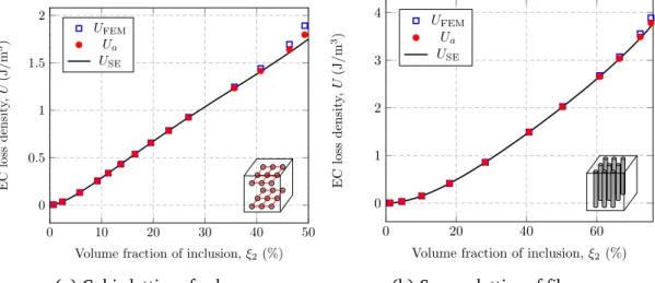
2.9 EC loss density as a function of inclusion volume fraction evaluated by full FEM computation (squares), by approximation (2.18) using the average magnetic field obtained by FEM (circles) and by the proposed analytical formulation (line). (a) case 1: Cubic lattice of spheres: magnetic field loading along z-direction, (b) case 2: Square lattice of fibers: in-plane loading field along y-direction. For all calculations: frequency f = 100 Hz, lattice size L1 = 50 µm, µ2 = 4000 µ0, µ1 = µ0,σ2 = 1.12 × 107S/m, average flux density B0= 1 T. . . 38 2.10 Errors on EC losses of the proposed homogenization model as a function

of volume fractionξ₂ for different frequencies. (a) case 1: Cubic lattice of spheres: magnetic field loading along z-direction, (b) case 2: Square lattice of fibers: in-plane loading field along y-direction. For all calculations: lattice size L₁= 50 µm, µ2 = 4000µ0,µ₁= µ0,σ₂ = 1.12 × 107_{S/m, average flux} density B₀= 1 T . . . 40

2.11 Errors on EC losses attributed to the average field assumption in equation (2.18) as a function of volume fractionξ2 for different frequencies. (a) case 1: Cubic lattice of spheres: magnetic field loading along z-direction, (b) case 2: Square lattice of fibers: in-plane loading field along y-direction. For all calculations: lattice size L1 = 50 µm, µ2 = 4000µ0, µ1 = µ0,σ2 = 1.12× 107_{S/m, average flux density B}

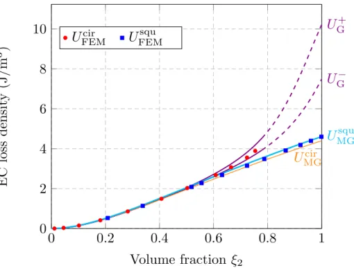
0 = 1 T. . . 40 2.12 EC loss densityU_SE evaluated with the proposed approach (lines) for cases

1 and 2 and corresponding FEM results U_FEM (dots) as a function of the permeability contrast between matrix and inclusions. For all calculations:

f = 100Hz, lattice size L1 = 50 µm, R = 24 µm, µ1 = µ0, σ2 = 1.12 × 107S/m, average flux density B0= 1 T. . . 42

List of figures xiii

2.13 Errors on EC losses of the proposed homogenization model as a function of the permeability contrast between matrix and inclusions for cases 1 and 2. Configuration: the same as Fig.2.12. . . 43

2.14 EC loss density versus different inclusion size. The filling factor is fixed for each case: 46.32 % for case 1 and 72.38% for case 2. For all calculations:

f = 100Hz, µ1 = µ0,µ₂ = 4000µ0, σ₂ = 1.12 × 107_{S/m, average flux} density B₀= 1 T. . . 44

2.15 Errors on EC losses of the proposed homogenization model as a function of the inclusion size for cases 1 and 2. Configuration: the same as Fig.2.14. . 44

3.1 Sketch of SMC in a 2D problem with in-plane magnetic field loading. . . 53

3.2 Spherical coordinates(r, θ, φ). . . . 55

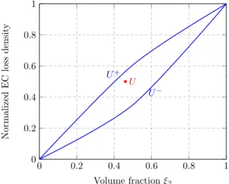
3.3 A schematic plot of EC loss density bounds as a function of volume fraction of the inclusion. . . 58

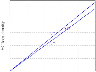
3.4 A schematic plot of EC loss density bounds as a function of permeability contrast. . . 59

3.5 A schematic plot of EC loss density bounds as a function of frequency. . . . 59

3.6 EC loss density as a function of filling factor of the inclusion. For all cal-culations: f = 100 Hz, lattice size L1 = 50 µm, µ2 = 4000 µ0,µ1 = µ0,

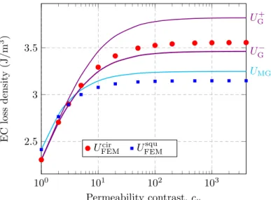
σ2= 1.12 × 107 S/m, average flux density B0= 1 T. . . 62 3.7 EC loss density as a function of the permeability contrast. Parameters: f =

100 Hz, lattice size L₁ = 50 µm, ξ2= 72.38%, µ1= µ0,σ₂= 1.12×107_S/m, average flux density B₀= 1 T. . . 64

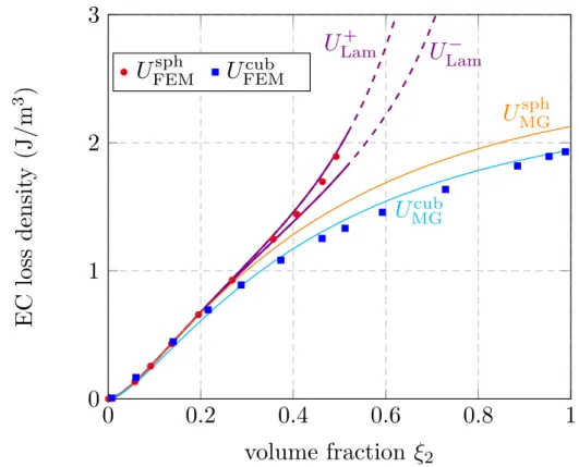
3.8 EC loss density as a function of the filling factor of the inclusions. Parameters:

f = 100 Hz, lattice size L1 = 50 µm, µ2 = 4000 µ0,µ₁ = µ0,σ₂ = 1.12 × 107_{S/m , average flux density B}

0= 1 T. . . 66 3.9 EC loss density as a function of the permeability contrast. For all calculations:

f = 100 Hz, lattice size L1 = 50 µm, ξ2 = 46.32%, µ1 = µ0,σ2 = 1.12 × 107_{S/m, average flux density B}

0= 1 T. . . 67 3.10 An example of SMC with random distribution of same-size cylinders. . . 68

3.11 EC loss density and the corresponding bounds. Disk size: R = 18 µm, Disk count: 16. L1 = 200 µm, f = 100 Hz, µ2 = 4000µ0,µ1 = µ0, σ2 = 1.12× 107S/m, average flux density B0 = 1 T . . . 69 3.12 Cross-sectional microscopic view of SMCs . . . 70

3.13 Comparison of EC loss density from different models with experimental results. (Sinusoidal polarization, peak value: 1 T). ‘Experimental’ results are from [91]; ‘distribution’ results are the prediction from [73] considering

the distributions of cross sections. . . 70

4.1 Sketch of periodic high concentration SMC. The domain confined by dashed lines 1-4 forms an elementary cell of the periodic pattern. . . 75

4.2 Flux density and eddy current density norm distribution in the inclusion. Lattice size L1= 50 µm, volume fraction ξ2= 97.6%, µ2= 4000µ0,µ1 = µ0,

σ2= 1.12 × 107S/m, average flux density B0 = 1 T, frequency f = 100 Hz. 77 4.3 Ratio of standard deviation of flux density to the average flux density norm

in the inclusion as a function of the filling factor. Lattice size L1= 50 µm,

µ2= 4000µ0,µ1= µ0,σ2= 1.12 × 107S/m, average flux density B0 = 1 T, frequency f = 100 Hz. . . 77

4.4 Effective permeability (real component) from MG estimate by comparing to FEM results, and the corresponding discrepancy. (2D SMC, cross-section magnetic permeability). Lattice size L1 = 50 µm, µ2 = 4000µ0, µ1 = µ0, magnetostatics. . . 79

4.5 EC loss density from complex permeability (MG) by comparing to FEM results, and the corresponding discrepancy. Lattice size L₁= 50 µm, µ2= 4000µ0,

µ1 = µ0,σ2 = 1.12 × 107S/m. The applied field is along y-axis, and the average flux density B₀= 1 T, frequency f = 100 Hz. . . . 80

4.6 Sketch of a schematic magnetic circuit made of SMC with square inclusions. The domain confined by red dashed lines forms an elementary cell of periodic pattern. . . 81

4.7 Geometry of the heterogeneous magnetic circuit calculated. . . 81

4.8 Geometry of equivalent virtual material (EVM) calculated. The red line in the gap is the cutline to examine the magnetic field distribution. . . 82

4.9 Magnetic field distributions on the homogeneous magnetic circuit. Relative Permeability: 48.9− j4.2 × 10−3_{, electric conductivity: 0. Frequency: 100 Hz. 83} 4.10 H_y distribution comparison for magnetic circuit made of SMC (blue dashed

line) and the homogeneous one (red line) and the corresponding errors. Parameters: same as the Fig.4.9. . . 84

4.11 EC loss density (mJ/m3_{) distribution on the heterogeneous magnetic circuit. 84} 4.12 Distribution of the errors on the EC losses over the magnetic circuit cells,

obtained by comparison between homogenization results and full field FEM calculation. . . 85

List of figures xv

4.13 EC loss error distribution of homogeneous magnetic circuit by comparing with the heterogeneous one. The color bar indicates the error values (%). The labels of the map are the dimensions of the magnetic circuit (in unit: µm) 86

5.1 Sketch of cubic lattice of cubic inclusions. The domain confined by its surrounding matrix (in red cube) forms an elementary cell of periodic pattern. 93

5.2 Magnetic flux density distribution in the inclusion. Lattice size: 50µm, volume fractionξ = 96%, µi= 4000µ0,σi = 1.12 × 107S/m, average flux

density B0= 1 T, frequency f = 100 Hz. . . . 93 5.3 Ratio of standard deviation of flux density to the average flux density norm

in the inclusion as a function of the filling factor. Lattice size: 50µm,

µi = 4000µ0,σi = 1.12 × 107S/m, average flux density B0= 1 T, frequency

f = 100 Hz. . . 94

5.4 Flow chart for the modeling scheme . . . 95

5.5 Average stress in the inclusion from MT estimate (5.9) by comparison to FEM results, and corresponding discrepancy. Lattice size: 50µm. T11= 1 MPa The mechanical parameters are listed in Tab.5.1. . . 96

5.6 Effective permeability (real component) from MG estimate by comparing to FEM results, and the corresponding discrepancy. Lattice size: 50µm, µ_i = 4000µ0. . . 97 5.7 Parallel component of the permeability of the inclusion as a function of

macroscopic stress Ta. Lattice length= 50 µm, volume fraction of inclusion

ξ = 99%. Material parameters as in Tab.5.1. . . 100

5.8 Parallel component of the effective relative permeability as a function of macroscopic stress Ta. Lattice length= 50 µm, volume fraction of inclusion

ξ = 99%. Material parameters as in Tab.5.1. . . 101

5.9 Experimental secant susceptibility under mechanical loadings[95]. . . 102

5.10 Normalized EC loss density as a function of macroscopic stress Ta. (Fixed

flux density B₀). Parameters: the same as Fig.5.7 . . . 102

5.11 Parallel component of the permeability of the inclusion as a function of Ta

for certain proportional coefficients. Parameters: the same as Fig.5.7 . . . . 104

5.12 Effective permeability (parallel component) as a function of Ta for certain

proportional coefficients. Parameters: the same as Fig.5.11 . . . 105

A.1 Sketch of homogeneous structure . . . 120

A.2 EC loss density in a homogeneous square as a function of frequency. σ = 1.12× 107 S/m, permeability µ = 4000µ0; Average flux density: 1 T. . . 123

A.3 Discrepancies between EC loss density by the linear fitting equation (A.24) and the reference values from (A.22). . . 124

A.4 Distribution of normalized eddy current density of a circle along a radius (red cut line in (b)). Radius: R= 25 µm . . . . 125

A.5 Normalized eddy current density (and the corresponding errors) as a function of the ratio between skin depth and size. . . 126

B.1 Phase shift betweenBandH, forming an ellipse in a period time. The area of this ellipse is the energy density during one time-period. . . 129

C.1 Sketch of the cubic lattice of spherical inclusions. . . 131

Résumé en Français

Le développement d’appareils légers, solides et peu énergivores est naturellement préférable. Dans les applications du génie électrique, les moteurs et les transformateurs utilisent des noyaux magnétiques afin de canaliser spatialement et de façon optimale le flux magné-tique. Les performances de telles machines dépendent grandement des propriétés du noyau magnétique utilisé. Le noyau magnétique est généralement conçu à partir de matéri-aux ferromagnétiques qui, malheureusement, sont aussi de bons conducteurs électriques. Lorsqu’un conducteur est placé dans un champ magnétique alternatif, des courants de Foucault (EC – Eddy Current) naissent, entraînant des pertes Joule dans le matériau. Dans la conception et l’analyse des machines électriques, la perméabilité magnétique et les pertes sont les deux caractéristiques dominantes à prendre en considération. Les matériaux composites permettent de réaliser des matériaux combinant les attributs des différents constituants pour fournir les caractéristiques souhaitées qui ne peuvent pas être facilement obtenues à partir de l’un ou l’autre des composants individuels.

Les composites magnétiques doux (SMC – Soft Magnetic Composites), généralement composés d’inclusions ferromagnétiques intégrées dans une matrice polymère diélectrique, présentent des pertes EC faibles tout en ayant une perméabilité magnétique relativement élevée. La matrice diélectrique confine les courants de Foucault dans chaque particule, réduisant ainsi considérablement les pertes EC du composite. Une autre particularité des SMC est l’isotropie magnétique et thermique[1,2], ce qui les rend adaptés à la construction

de dispositifs électriques à structure complexe, avec des flux magnétiques tridimensionnels - en comparaison avec les structures laminées classiques. Les SMC présentent ainsi un fort potentiel pour une utilisation dans l’industrie aérospatiale, maritime et automobile en remplacement des matériaux ferromagnétiques traditionnels[3–9]. La recherche continue

sur les SMC a montré une large gamme d’applications dans la conception de moteurs[10],

tel que les moteurs à aimants permanents à flux transversal[11–13], les moteur à aimants

permanents à flux axial[14] pour les véhicules électriques hybrides ainsi que les moteurs à

induction[15]. Les SMC sont normalement fabriqués à partir de techniques issues de la

d’une matrice diélectrique pour réduire les courants de Foucault globaux et les confiner dans chaque particule. Les particules de poudre sont généralement de forme irrégulière, avec un diamètre moyen d’environ 50 à 250µm. Les matériaux ferromagnétiques généralement sélectionnés sont du fer pur ou des alliages à base de fer, tels que les alliages Fe-Ni (haute perméabilité), les alliages Fe-Si (résistivité électrique élevée) et les alliages Fe-Co (haute saturation magnétique) [3]. Une forte concentration d’inclusions magnétiques donne

une densité plus élevée, une bonne résistance mécanique et une perméabilité magnétique élevée du composite. Les matériaux de revêtement peuvent être inorganiques ou organiques. L’époxy est souvent choisi comme matériau matriciel. Une fraction de revêtement plus élevée réduira considérablement les pertes EC, mais la performance magnétique globale sera alors diminuée. L’équilibre entre ces caractéristiques (perméabilité versus pertes) doit donc être pris en compte dans la conception de SMC.

L’étude des propriétés effectives des matériaux composites fait l’objet d’un vaste effort de recherche[17–25]. L’idée principale est de remplacer la microstructure du

compos-ite par un matériau homogène équivalent, qui peut ensucompos-ite être utilisé dans des outils d’analyse structurale standard, avec une complexité numérique réduite. Différents modèles analytiques et numériques ont été proposés.

Les techniques d’homogénéisation par la Méthode des éléments finis (FEM)[26–29]

ont été introduites pour aborder ce type de problèmes électromagnétiques à différentes échelles. Diverses stratégies ont été proposées [30, 31] pour réduire le temps et les

ressources de calcul dans une certaine mesure tout en maintenant la précision. Néanmoins, ces méthodes numériques ont souvent l’inconvénient d’être peu flexibles, par exemple pour des études paramétriques nécessitant de multiples calculs numériques. En outre, il est difficile de considérer les problèmes avec des contrastes élevés en propriété, nécessitant souvent un maillage raffiné, à moins que des techniques numériques spécifiques ne soient utilisées[31,32].

Ainsi, il est crucial de développer de nouveaux modèles pour les pertes EC dans les SMC. D’autres approches basées sur des formulations analytiques et semi-analytiques ont égale-ment été étudiées. Les approches en champ moyen ont par exemple été développées pour déterminer la perméabilité magnétique effective des polycristaux ferromagnétiques[33,34].

Des stratégies d’homogénéisation analytiques ont également été utilisées pour déterminer la permittivité effective de composites pour des applications de blindage électromagné-tique[35–37]. Puisque les échelles de la taille des grains et la taille typique du dispositif

sont bien séparées, ces stratégies d’homogénéisation sont un choix pertinent pour les SMC. En électromagnétisme, les techniques d’homogénéisation sont utilisées pour déterminer les propriétés électriques et magnétiques effectives des matériaux. La monographie de

Si-Résumé en Français xix

hvola[23] donne un aperçu utile des techniques d’homogénéisation pour les comportements

des matériaux en régime quasistatique.

Les propriétés effectives sont définies comme le tenseur des propriétés reliant les champs duaux macroscopiques. A partir de lois de comportements locales (propres à chaque constituant) reliant les champs duaux locaux (par exemple le champ magnétique H et l’induction magnétique B, reliés par le tenseur de perméabilitéµ), et à travers des opérations de moyenne volumique, les propriétés effectives d’un matériau composite peu-vent être obtenues. Une approche simplifiée des problèmes d’homogénéisation peut être utilisée avec les approches en champs moyens. Celle-ci se contente d’une quantité lim-itée d’informations sur la microstructure (fractions volumiques et quelques indicateurs statistiques). Dans les cas pratiques, une connaissance complète de la microstructure des composites n’est pas nécessairement disponible, et les propriétés effectives pour le matériau homogène équivelent (EHM – equivalent homogeneous medium) ne peuvent être exacte-ment déterminées. Néanmoins, les formules d’homogénéisation permettent de fournir des estimations ou des bornes du comportement effectif à partir des informations connues sur la microstructure. Considérons par exemple un composite biphasé avec des inclusions placées dans une matrice. La perméabilité effective d’un tel matériau se situe nécessairement entre les limites inférieures et supérieures fournies par les bornes de Wiener [19]. Des

limites plus étroites peuvent être obtenues si l’information d’isotropie globale du matériau est considérée, menant aux bornes de Hashin-Shtrikman[20,38]. Fournir des bornes du

comportement effectif peut être insuffisant tant l’écart entre les bornes peut parfois être large. Il est alors utile de fournir une estimation du comportement effectif. Le formalisme de Maxwell-Garnett (MG) a été présenté en 1904 pour estimer la permittivité effective d’un EHM diélectrique isotrope pour un matériau composite fabriqué à partir d’une dispersion de particules sphériques dans un matériau hôte [18]. Ce modèle est particulièrement

valide pour les composites à faible fraction volumique d’inclusions (matériaux dilués). C’est l’une des méthodes les plus utilisées pour calculer les propriétés macroscopiques des matériaux non homogènes[39–44]. L’estimation de MG est identique à la limite inférieure

de Hashin-Shtrikman. Un autre modèle, celui de Bruggeman[45] permet de fournir une

estimation plus pertinente pour les matériaux non dilués. Les matériaux constitutifs du matériau composite sont alors considérés comme jouant des rôles similaires (plus de dis-tinction matrice/inclusion). En réalité, dans le modèle de Bruggeman, on suppose que les phases constitutives sont dispersées dans l’EHM lui-même. Les estimations des propriétés effectives dépendent alors seulement des propriétés des matériaux constitutifs et de leurs fractions volumiques. Le principal avantage de ces modèles réside dans leur simplicité relative (modèles analytiques ou quasi-analytiques).

Dans le cas de microstructures périodiques, la technique d’expansion asymptotique [26–29,46] peut être utilisée. Parmi les méthodes alternatives, des expériences sur des SMC

commerciaux ou des prototypes ont été menées pour étudier les propriétés magnétiques et les caractéristiques des pertes[47–49]. Mais les approches expérimentales ne conviennent

pas aux processus de conception en raison des contraintes de coût et de temps.

Par conséquent, dans la phase de conception, les formules analytiques sont fortement préférées, permettant de relier de façon directe les propriétés des constituants, la mi-crostructure et les performances attendues. De ce fait, les stratégies d’homogénéisation (quasi-)analytiques sont préférables pour les stades de conception.

Une considération supplémentaire est nécessaire pour étudier les SMC de façon perti-nente. En effet, le comportement magnétique des matériaux ferromagnétiques est générale-ment sensible à l’application d’une contrainte mécanique[50–52]. Le couplage

magnéto-mécanique peut être principalement décrit par deux aspects. L’un est la magnétostric-tion [53], décrivant la déformation de matériau sous l’effet d’un champ magnétique.

L’autre est l’effet de la contrainte sur le comportement magnétique [54], représentant

le changement de susceptibilité magnétique en fonction de la contrainte. Ces comporte-ments peuvent être décrits par des approches phénoménologiques[55,56] ou des modèles

multi-échelles[57–59]. L’analyse des pertes dans les matériaux ferromagnétiques [60–62]

ainsi que le couplage magnéto-mécanique[58,63,64] ont menés à de nombreuses études

sur ces matériaux, tant d’un point de vue expérimental qu’en termes de modélisation. Un modèle analytique a été proposé pour décrire la dépendance de la susceptibilité magnétique à la contrainte[65]. Néanmoins, il n’existe pas de modèle précis pour prendre en compte

l’effet des contraintes mécaniques sur les pertes.

Cette thèse est consacrée au développement de modèles analytiques ou semi-analytiques pour les pertes par courants de Foucault dans les composites magnétiques doux. L’examen détaillé de la distribution des champs magnétiques et électriques n’est pas la préoccupation principale. Dans la plupart des cas, on peut se contenter d’approximations raisonnables sur les champs pour déterminer les pertes par courants de Foucault d’un point de vue macroscopique. Les propriétés complexes peuvent être utilisées dans des applications électromagnétiques pour décrire les phénomènes dissipatifs. Un examen approfondi des modèles d’homogénéisation pour le comportement diélectrique utilisant la permittivité complexe peut être trouvé dans[42,66]. Les cas 2D et 3D ont été explorés numériquement

en détails. La permittivité complexe dépend des propriétés de chaque constituant, de leur fraction de volume et de leur répartition spatiale[67]. De manière analogue, la perméabilité

complexe est un outil utile pour traiter les effets magnétiques à haute fréquence, par exemple dans les applications de transformateurs[68,69]. La dissipation peut se refléter directement

Résumé en Français xxi

dans la partie imaginaire de la perméabilité complexe [70, 71]. Dans le cas de SMC à

basse fréquence, lorsque le champ magnétique induit peut être négligé, il n’y a pas de déphasage entre la densité de flux magnétique et le champ magnétique. À cet égard, la partie imaginaire de la perméabilité complexe doit être considérée comme nulle. Toutefois, les pertes EC sont présentes - tant que la fréquence n’est pas nulle. Ainsi, une partie imaginaire peut être introduite dans le tenseur de perméabilité magnétique de manière à refléter les pertes EC.

Le tenseur de perméabilité complexe peut être utilisé comme un outil mathématique pour représenter un matériau magnétique dissipatif. Dans cette étude, ce tenseur de perméabilité complexe est utilisé pour décrire les performances électromagnétiques des SMC. La partie réelle est la perméabilité effective, et la partie imaginaire reflète les pertes EC. Les modèles développés se basent sur l’étude de composites à microstructure périodique avec des inclusions circulaires ou sphériques excités par des champs magnétiques harmoniques. Si, comme c’est en général le cas, le champ dans l’inclusion n’est pas uniforme, on considère alors les champs moyens dans les différentes phases. La perméabilité complexe est une propriété matériaux, indépendante de la géométrie. Elle peut être utilisée comme une propriété constitutive dans la conception de machines utilisant des SMC. Sur la base de l’étude d’une seule inclusion dans un milieu infini, on déduit les propriétés de matériaux hétérogènes dilués et le cas général des composites est extrapolé à partir de cette approche. La densité de pertes EC dans les SMC est ensuite décrite à l’aide du tenseur de perméabilité complexe homogénéisé. L’approche est comparée aux résultats obtenus par un modèle éléments finis et les erreurs observées restent généralement inférieures à 5%. Il convient de noter que l’approche nécessite des estimations précises du tenseur de perméabilité magnétique statique efficace du matériau composite. C’est généralement la principale difficulté d’un tel modèle. On constate que l’approche tend à sous-estimer la densité de pertes EC par rapport aux résultats éléments finis et que les erreurs sont indépendantes de la fréquence sous l’hypothèse de basse fréquence.

La densité de pertes EC dans les SMC peut être approchée en estimant le champ magnétique soit à partir des moments de premier ordre (moyenne classique pour obtenir le champ moyen) soit à partir des moments du second ordre (moyenne des carrés du champ magnétique) du champ magnétique. Pour les SMC périodiques avec des inclusions circulaires ou sphériques, il a été prouvé dans cette étude que les deux approches permettent de borner les pertes EC. L’approche utilisant la moyenne du champ magnétique sous-estime la densité de pertes EC dans les SMC, fournissant ainsi une limite inférieure; alors qu’elle est surestimée dans l’approche utilisant les moments d’ordre deux, fournissant ainsi une limite supérieure. Les deux estimations sont généralement proches l’une de l’autre, fournissant

des valeurs précises pour les pertes EC tant que la perméabilité efficace est estimée avec une bonne précision. Les pertes EC peuvent ainsi être approchées, sans connaissance de la solution exacte de la distribution d’EC, ce qui simplifie l’approche par rapport à un calcul FEM complet. Quand la perméabilité effective n’est pas connue mais estimée, les pertes calculées perdent leur propriété de borne et sont simplement des estimations.

Comme exemple d’application, un circuit magnétique constitué de SMC est homogénéisé avec la méthode de la perméabilité complexe. Il est composé de SMC à haute concentration à microstructure périodique. Des calculs FEM ont été effectués sur la structure hétérogène et sur la structure avec le matériau homogène équivalent. Les répartitions du champ magnétique et des pertes EC ont été examinées et comparées entre les deux solutions. Un bon accord est observé entre la densité de pertes EC de référence (obtenue pour le transformateur hétérogène) et les valeurs calculées avec une perméabilité complexe. Les calculs montrent que l’erreur globale sur les pertes EC est très faible (moins de 0,5%) et les erreurs locales ne dépassent pas 3% généralement, sauf pour des zones très localisées du circuit (angles droits de la géométrie). On conclut alors que la méthode d’homogénéisation peut fournir une répartition des pertes EC avec une précision très satisfaisante.

En plus de cela, le comportement multi-physique des SMC est exploré. L’effet de la contrainte mécanique sur la performance magnétique et sur la densité des pertes EC est étudié pour les SMC à concentration d’inclusions ferromagnétiques élevée. A partir des perméabilités locales, et en négligeant la magnétostriction, une formule est dérivée pour la densité de pertes EC en fonction du champ magnétique macroscopique et de la contrainte mécanique. La contrainte a une influence sur la densité de pertes EC en raison de la variation du comportement magnétique du matériau ferromagnétique sous contrainte. Il est montré que la contrainte a peu d’effet sur les pertes EC dans les SMC (tout en affectant la perméabilité magnétique). On en tire une conclusion intéressante : le comportement magnétique des SMC semble être moins sensible à la contrainte mécanique que celui des matériaux ferromagnétiques homogènes habituels. Cette attente doit être confirmée par des mesures expérimentales. Dans cette étude, les pertes par hystérésis et la non linéarité du comportement ne sont pas prises en considération. Pour un comportement magnétique non-linéaire, le modèle serait bien plus complexe à mettre en œuvre. Puisque la perméabilité magnétique dépend dans ce cas du champ magnétique appliqué, une procédure itérative devrait être utilisée pour obtenir le champ moyen dans l’inclusion, puis le tenseur de perméabilité de l’inclusion, et enfin le tenseur de perméabilité effective du composite. En outre, le champ magnétique harmonique doit être échantillonné au fil du temps afin de déterminer le champ moyen final et la perméabilité de l’inclusion. La densité de pertes EC doit ensuite être intégrée sur une période de temps.

Résumé en Français xxiii

Les modèles développés ici proposent des approches directes pour déterminer les pertes EC dans les SMC à faible fréquence de travail. La perméabilité complexe contient le comportement magnétique ainsi que les pertes EC. Les approches menant aux bornes des pertes EC offrent un moyen simple de se rapprocher des pertes EC dans le composite. L’effet de la contrainte mécanique est également directement intégré dans la formule de densité de pertes EC. Les modèles sont adaptés à différents contrastes de perméabilité et sont discutés pour une gamme complète de fractions volumiques. Ils sont développés pour les SMC ayant une matrice diélectrique. Lorsque les courants de Foucault globaux dans la matrice ne peuvent plus être négligés, les modèles doivent être corrigés. Les formules de densité de pertes EC sont dérivées à partir des SMC à microstructure périodique. Pour des SMC avec des microstructures aléatoires, des estimations des pertes EC peuvent également être obtenues. Dans cette étude, la non-linéarité des matériaux ferromagnétiques, l’hystérésis et les pertes par excès ne sont pas pris en compte.

En conclusion, cette étude fournit une méthodologie pour obtenir une perméabilité complexe décrivant le comportement de matériaux ferromagnétiques linéaires. Cette méthodologie donne un accès simple aux pertes par courant de Foucault. Les perspectives à ces travaux seront de développer un modèle de perméabilité complexe générique intégrant la non-linéarité du comportement magnétique, ainsi que l’hystérésis et les pertes par excès. De plus, il serait intéressant d’intégrer un couplage magnétomécanique fort dans le modèle de la perméabilité magnétique complexe. Des expériences sont nécessaires pour valider les modèles. Le couplage magnétomécanique est souvent négligé dans les études sur les SMC, ces travaux montrent néanmoins que les contraintes mécaniques ont un effet sur le comportement des SMC. L’effet de la température sur les propriétés électromagnétiques pourrait également être pris en compte. Une formule générique pourrait être développée pour faire face aux comportements couplés des SMC en utilisant des techniques d’homogénéisation. Les travaux futurs pourraient également inclure l’application du modèle de perméabilité complexe dans les outils de dimensionnement de structure pour concevoir des moteurs et des transformateurs à base de SMC. Les dispositifs prototypes pourraient être développés et fabriqués et les performances électriques comparées à celles des machines traditionnelles. Promouvoir l’application de SMC en remplacement de l’acier stratifié dans les appareils électriques afin d’économiser de l’énergie sera une tâche difficile mais importante.

General Introduction

Industrial development relies a lot on lighter, stronger and more energy efficient devices. Motors and transformers are widely used in Electrical Engineering applications. The fundamental component of a static or rotating device is its magnetic core, designed to amplify and to control the direction of the magnetic flux that in turn determines a machine’s performance. This function requires a high saturation magnetization. The magnetic core is designed with ferromagnetic materials, which, unfortunately, are generally highly conductive. When a conductor experiences an alternative magnetic field, eddy currents (EC) circulate, resulting in losses. In the design and analysis of electrical machines, magnetic performance and losses are the two dominant points to be taken into consideration.

Composite materials offer a balance between the two points. Composites combine the attributes of constituents to provide desired features which cannot readily be obtained from either of the individual components. Soft Magnetic Composites (SMC), typically composed of ferromagnetic inclusions embedded in a dielectric polymer matrix, possess the characteristics of low level of EC losses when they are subjected to electromagnetic loadings. SMC have the potential for widespread usage in aerospace, naval and automotive industries as a perspective replacement to traditional metal materials owing to designable magnetic and thermal properties and comparatively low EC losses[3–9].

In order to design electrical machines using SMC as the magnetic material, the opti-mization of material properties is crucial. First, a high magnetic permeability is required. Pure iron or Fe-alloys are then good candidates for the particle material. Second, low EC losses are needed and can be achieved thanks to the dielectric coating which significantly cuts down the induced EC. Epoxy is often chosen as the matrix material. These constituents exhibit a very high contrast both in electric conductivity and magnetic permeability. This high property contrast is a serious challenge for homogenization techniques developed in order to deduce the effective properties of heterogeneous materials. However, these homogenization techniques are required to design optimal electromagnetic devices based on SMC.

The study of the effective property of composite has been a large area of research[17–

25]. Analytical and numerical models were proposed. Powerful computing capacity enabled

the rapid development of numerical strategies. One of the most commonly employed is the Finite Element Method (FEM). FEM provides a full-field approach to electromagnetic problems. Effective properties and losses can then be post-processed. But in the case of SMC, the microstructure has to be finely meshed, which brings significant numerical burden and instabilities in FEM approach. FEM homogenization techniques[26–29] have been

introduced to tackle electromagnetic problems with different scales. The main idea is to replace periodic microstructures of the composite by an equivalent homogeneous material, which can then be used in standard structural analysis tools, with a reduced numerical complexity. Various strategies derived from standard FEM have been proposed[30,31].

These methods reduce the computational time and resources to a certain extent while maintaining accuracy. Nevertheless, these numerical methods still have the drawback of being not very flexible, for instance for parametric studies that require multiple numerical computations. Also, it is difficult to address the problem of high property contrast unless specific numerical techniques are used[31,32]. Thus, it is crucial to develop new models

for EC losses in SMC.

On the other hand, analytical and semi-analytical approaches are widely studied. Mean field methods have for instance been developed for the determination of the effective magnetic permeability of ferromagnetic polycrystals[33,34]. Analytical homogenization

strategies have also been used for the determination of the effective permittivity of com-posites for shielding applications[35–37]. These analytical or semi-analytical models pour

attention only on the effective constitutive properties and do not provide an insight into losses characteristics of composites.

Among alternative methods, experiments on commercial SMC or prototypes have been conducted to study the magnetic properties and lossy characteristics[72–74]. But

experimental approaches are not suitable for design processes due to the cost and time constraints.

Therefore, in the phase of design, analytical formulas are greatly required, by which the selection of constituents can be easily realized for the desired performance. Thus a constitutive study of SMC is critically important. In addition, at this stage, the overall performance and the balance between properties are the utmost concerns. Therefore homogenization strategy is thus a preferable choice for this constitutive study.

In addition, the magnetic behavior of ferromagnetic materials is usually sensitive to the application of mechanical stress[50–52]. Ferromagnetic material loss analysis [60–62] and

3

respective branches. An analytical model has been proposed to describe the dependence of the magnetic susceptibility to stress[65]. Still, there is no accurate model to take care of

the loss characteristics under mechanical stress applications. For SMC, since the matrix is nonmagnetic and dielectric, the magneto-mechanical coupling in the ferromagnetic inclusion is of concern.

This thesis is devoted to developing analytical or semi-analytical models for eddy current loss in soft magnetic composites. Detailed examinations of the magnetic and electric field distributions are not the most crucial concern, and in most cases, some reasonable approximations of the field are enough to determine the eddy current loss from a macroscopic point of view. In this thesis, homogenization techniques are applied to determine the magnetic permeability and EC losses of SMC.

Outline of the manuscript

This present thesis is elaborated in five chapters:

The first chapter introduces Maxwell’s equations, constitutive relations, the concept and characteristics of Soft Magnetic Composites, and homogenization strategies.

In chapter2, a complex permeability is proposed to characterize both the magnetic behavior (real component) and loss characteristic (imaginary component). This complex permeability is deduced based on an average field approach.

In chapter3, EC loss bounds are analytically derived for simple geometries.

Chapter4provides an application example. A transformer made of high concentration SMC is considered. The complex permeability model is applied to the calculation of the transformer.

Chapter5consists in a discussion of the effect of stress on the magnetic performance and EC losses of SMC. EC loss density as a function of macroscopic stress and magnetic field is presented.

Chapter 1

Basic Equations for the Modeling of Soft

Magnetic Composites

Contents

1.3 Eddy Current Losses . . . . 13

1.3.1 EC Loss Density Definition . . . 13

1.3.2 EC Loss Density of Homogeneous Structures . . . 14

1.4 Soft Magnetic Composites . . . . 15

1.4.1 EC Loss Density of SMC . . . 17

1.5 Homogenization Techniques . . . . 17

1.1 Maxwell’s Equations 7

In order to understand the electromagnetic behavior of Soft Magnetic Composites (SMC), it is necessary to take into consideration the constitutive behavior of different

phases of the composites.

The aim of this chapter is to synthesize the theoretical formulas to model the electromag-netic behavior of SMC. Maxwell’s equations are first introduced. The boundary conditions are derived at the interface, which express the continuity of electromagnetic fields across the boundary between two media. Material constitutive relations are introduced in sec-tion 1.2. The eddy current (EC) loss density is then defined for conductive materials. Formulas for EC loss density are deduced for simple homogeneous structures and simplified at low frequency in section1.3. An introduction on Soft Magnetic Composites is given in section1.4. The final section presents homogenization techniques for the determination of effective properties of composite materials.

1.1

Maxwell’s Equations

Electromagnetic (EM) theory can be regarded as the study of fields produced by electric charges at rest and in motion. Dynamic or time-varying fields are usually due to accelerated charges or time-varying currents[75]. Electromagnetism studies the coupling phenomenon

between the electric field and magnetic field. The pioneering physicists, Ampère and Faraday, among others, conducted experiments on electricity and magnetism. These experimental observations were summed up by James Clerk Maxwell in four mathematical formulas[76–78]: ∇ × E = −∂ B ∂ t Maxwell-Faraday ∇ × H = J +∂ D ∂ t Maxwell-Ampère ∇ · D = ρ Gauss electric ∇ · B = 0 Gauss magnetic (1.1a) (1.1b) (1.1c) (1.1d) whereρ (C/m3) represents the volume density of free electric charges. The four fields E, H,

B, and D are respectively the electric field(V/m), the magnetic field (A/m), the magnetic

flux density(T) and the displacement flux density (C/m2). J (A/m2) is the electric current density. Maxwell’s equations are first-order linear coupled differential equations relating the vector field quantities to each other. They unify the four fields E, H, B, and D in a system of partial differential equations. The charge densityρ and the current density J

comply with the continuity equation,

∇ · J +∂ ρ

∂ t = 0 (1.2)

which expresses the conservation of the electric charge. Equations (1.1a)–(1.1d) are solved in a bounded subdomainΩ of the Euclidean space R3_.

Ω2

Ω1

Γ

Fig. 1.1 Boundary condition at the interface between two material domainsΩ1 andΩ2 The interfaceΓ separates two different materials Ω₁ andΩ₂, shown in Fig.1.1. Elec-tromagnetic fields can be discontinuous at the interface. The fields in Ω1 and Ω2 are distinguished by the subscript 1 and 2, respectively. A unit normal vector n is directed from

Ω1 to Ω2. Denote the surface current density vector K and surface charge densityρS on

the interfaceΓ . The boundary conditions can be easily deducted from the integral form of Maxwell equations. They are[75,77]

onΓ ,            (E1− E2) × n = 0 (H1− H2) × n = K (D1− D2) · n = ρS (B2− B1) · n = 0 (1.3a) (1.3b) (1.3c) (1.3d) These equations show the continuity of the tangential component of E (1.3a) and of the normal component of B (1.3d) whereas the tangential component of H (1.3b) and the normal component of D (1.3c) are discontinuous respectively by K andρ_S on the boundary.

1.2

Constitutive Relations

The distribution of electromagnetic fields also depend on the medium properties character-ized by the constitutive parameters: magnetic permeabilityµ (H/m), electric conductivity

1.2 Constitutive Relations 9 σ (S/m) and dielectric permittivity ε (F/m). These properties are generally in the form of

second order tensor. These tensors are symmetric and therefore can be expressed with 6 coefficients: µ =   µ11 µ12 µ13 µ12 µ22 µ23 µ13 µ23 µ33   (1.4)

for the magnetic permeability tensor (the same form for the conductivity and permittivity tensors). For the isotropic case, the magnetic behavior is described by a scalarµ:

µ = µ I (1.5)

where I is the second order identity tensor.

The constitutive laws are the formulas that link the fields through the material properties:

B= µ · H D= ε · E J= σ · E (1.6a) (1.6b) (1.6c) These relations together with Maxwell equations (1.1) and well-posed boundary condi-tions close the electromagnetic problems.

1.2.1

Magnetic Behavior

In vacuum the constitutive magnetic law is:

B= µ0H (1.7)

withµ0= 4π × 10−7(H/m) the vacuum permeability. For linear magnetic materials with magnetic susceptibility tensor χ, the degree of magnetization M is proportional to the

magnetic field H by:

M= χ · H (1.8)

so that the magnetic constitutive relation is:

In the case of isotropic materials, the magnetic susceptibility does not depend on the direction of the external field. Thus it becomes a scalar quality (χ = χI). In vacuum,

χ = 0. Materials with small positive susceptibility are called paramagnetic. In this case, the

magnetic field in the material is strengthened by the induced magnetization. On the other hand, ifχ < 0, the material is diamagnetic. In this case, the magnetic field in the material is weakened by the induced magnetization. The susceptibility values of the paramagnetic and diamagnetic materials are small[52,79,80].

Ferromagnetic materials have a large positive susceptibility to an external magnetic field. They exhibit nonlinear behavior (susceptibility depends on the applied magnetic field) and possible hysteretic behavior, shown in Fig.1.2.

Br

Hc

Bs

H B

Fig. 1.2 Hysteresis loop (red curve) for a nonlinear irreversible magnetic material (the blue curve is the anhysteretic curve).

When a ferromagnetic material is magnetized in one direction, it will not relax back to zero magnetization when the imposed field is removed. The remaining flux density is called remanent induction Br. It must be driven back to zero by the coercive magnetic

field Hcin the opposite direction. As the imposed magnetic field increase, the flux density

reaches saturation Bs. According to the values of their coercive magnetic field, ferromagnetic

materials can be classified into two categories. Materials which maintain their magnetization and are difficult to demagnetize are called hard magnetic materials. These materials find their greatest use in permanent magnets. On the contrary, soft ferromagnetic materials have a small coercive magnetic field (typically less than 103A/m), which results in low amount of hysteresis loss. The constitutive relation for soft magnetic materials is roughly approximated by the anhysteretic curve[81,82]. For low level of magnetic field, the soft

magnetic material can be further approximated as linear, as shown in Fig.1.3. In this manuscript, the magnetic materials will be considered linear.

1.2 Constitutive Relations 11

B

H

linear

nonlinear

Fig. 1.3 BH curves for linear (red line) or nonlinear (blue curve) reversible magnetic material.

1.2.2

Mechanical Behavior

The mechanical behavior that links the strain tensor S (second-order) and the stress tensor T (second-order) has the form:

T = C : S (1.10)

whereC is a fourth-order stiffness (elasticity) tensor. Using Einstein notation, (1.10) writes:

T_{i j} = C_{i jkl}S_kl. The stiffness tensorC is a material property to represent the resistance to deformation in response to an applied force. It is constant in a linear elastic material. The stress tensor T is the force per unit area on a body [83].The intensity of distortion is known

as strain tensor S. It is a dimensionless tensor of rank 2.

Due to the inherent symmetries ofC (Ci jkl = Cjikl= Ci jl k= Cjil k = Ckl i j), the stiffness

tensor can be represented by a symmetric second order tensor. For orthotropic materials which have three orthogonal planes of symmetry, the stiffness tensor can be described by 9 independent parameters: Corth=          C11 C12 C13 0 0 0 C12 C22 C23 0 0 0 C13 C23 C33 0 0 0 0 0 0 C44 0 0 0 0 0 0 C55 0 0 0 0 0 0 C66          (1.11)

For isotropic media (which have the same physical properties in any direction), the stiffness tensor C can be reduced to only two independent numbers, the bulk modulus κ and the shear modulus G, that quantify the material’s resistance to changes in volume and to

shearing deformations, respectively. Ciso=          κ +4 3G κ − 2 3G κ − 2 3G 0 0 0 κ −2 3G κ + 4 3G κ − 2 3G 0 0 0 κ −2 3G κ − 2 3G κ + 4 3G 0 0 0 0 0 0 2G 0 0 0 0 0 0 2G 0 0 0 0 0 0 2G          (1.12)

In this work, the elastic property of material will be considered isotropic.

1.2.3

Magneto-Mechanical Behavior

The magneto-mechanical coupling can be principally described by two aspects: • Magnetostriction[53]: strain induced by magnetization.

• Effect of stress[54]: change of the magnetic susceptibility of a material when

sub-jected to a mechanical stress.

The corresponding behaviors are generally described by phenomenological approaches [55,56] or multi-scales models [57–59]. The magnetic behavior of ferromagnetic material

is sensitive to the application of mechanical stress[51,52]. Fig.1.4gives an example of

mag-−0.5 0 0.5 1 −1 −0.5 0 0.5 1 x 106 H (kA/m) M (A/m) σ = 0 −50 MPa −100 MPa

Fig. 1.4 Magnetization curves for a nonoriented Iron-Silicon alloy subjected to a uniaxial compression applied in the direction parallel to the magnetic field[84].

1.3 Eddy Current Losses 13

netization curves for a nonoriented Iron-Silicon alloy subjected to a uniaxial compression applied in the direction parallel to the magnetic field[84].

Consider a ferromagnetic material that is subjected to a magnetic field H in the direction

x(H = H x) and simultaneously a stress state T:

T =   T₁₁ T₁₂ T₁₃ T₁₂ T₂₂ T₂₃ T₁₃ T₂₃ T₃₃   (1.13)

An analytical magneto-elastic model has been proposed in[65]. The magnetization of the

ferromagnetic core can be written in the form:

M= A1sinh(κH)

A1cosh(κH) + A2+ A3

M_sx (1.14)

with

A_i= exp (αT_ii) , i = {1, 2, 3} (1.15) where M_s is the saturation of magnetization of the material. α and κ are material constants.

1.3

Eddy Current Losses

1.3.1

EC Loss Density Definition

Once the Maxwell’s equations are solved with constitutive laws and boundary conditions, the distribution of electric field E and magnetic field H can be obtained. In a conductorΩ of conductivityσ there arises eddy current Jeddy= σ · E, which results in EC losses in the material. In a harmonic electromagnetic problem, the EC loss densityU is defined as the Joule losses dissipated per unit volume during a wave period:

U = 〈E

∗_{·σ · E〉}

2 f (1.16)

where f is the working frequency. The superscript “*” refers to the conjugate transpose operator and the operator〈·〉 denotes a volume average over the domain Ω by 〈·〉 = _V1 R_V· dV , where V is the volume ofΩ.

The EC losses increase the temperature of the magnetic material. On the one hand, EC can be used in the case of induction heating. On the other hand, the heat represents a major source of energy loss in AC machines like transformers, generators, and motors. The

heat must be safely dissipated otherwise it would deteriorate the working performance or cause a risk of failure due to local overheating or thermal cycling.

1.3.2

EC Loss Density of Homogeneous Structures

Consider an isotropic, homogeneous and linear material of permeabilityµ, electric con-ductivityσ, and permittivity ε. The material is submitted to a harmonic magnetic field

H of frequency f (angle frequency: ω = 2π f ). Combining Maxwell’s equations with

constitutive laws of material, the problem becomes a Poisson equation,

∇ × ∇ × H = − jωµ( jω ε + σ)H (1.17) The definition of EC loss density in (1.16) is a general one. It applies for any frequency. Nevertheless, in the following formula derivation, quasistatics is assumed meaning that the frequency is low enough so that the induced magnetic field generated by the electric field can be ignored.

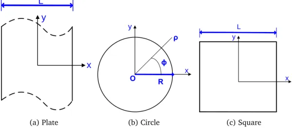
When a structure is homogeneous, Maxwell’s equations (1.1) can be analytically solved for some basic 2D shapes, for instance, a plate, a circle, and a square, as shown in Fig.1.5.

L

y

x

Fig. 1.5 Sketch of homogeneous structures

Since the domain is cut from 3D structure with infinite dimension along the z-axis, the magnetic field and the induced electric field are z-invariant,

∂ H

∂ z = 0

and

∂ E

1.4 Soft Magnetic Composites 15

Let’s apply a magnetic field H = [0, 0, Hz]t on the domain Ω, where the superscript t

indicates a matrix transpose, and consider a low frequency such thatωε ≪ σ. Denoting

k2= −jωµσ, the Poisson equation (1.17) becomes,

∇2_{H+ k}2_{H= 0 (1.19)}

subject to the Dirichlet boundary condition H|∂ Ω= Hz with∂ Ω denoting the boundary of

the domain. According to the boundary condition and z-invariance, and considering null current flow in the fiber, we have,

E_z = 0

and

To solve (1.19) in a domain of one of the basic shapes, shown in Fig.1.5, the magnetic field and electric field can be obtained. Therefore, the eddy current density has the form:

U_plate=1 6π 2 f σ µ2H_z2L2 Ucircle= 1 4π 2 f σ µ2H_z2R2 (1.21a) (1.21b) See AppendixAfor detailed derivations. As for the square-shaped material, a simple form as (1.21) can not be directly obtained. Nevertheless, since the proportional relationship holds[85,86]:

U ∝ f σ µ2_H2

z L

2_{, (1.22)}

the EC loss density of a square-shaped material can be approximated as: U_square= 9

128π 2

f σ µ2H_z2L2 (1.23)

See the detailed steps and the errors of this approximation in AppendixA.

1.4

Soft Magnetic Composites

Soft Magnetic Composites (SMC) consist of ferromagnetic inclusions embedded in a dielec-tric polymer matrix, as shown in Fig.1.6. The unique properties of SMC materials include magnetic and thermal isotropy[1,2], making them suitable for constructions of electrical

devices with complex structure and three-dimensional magnetic flux path. SMC have the advantages of low core losses and high magnetic permeability at various frequency ranges.