Online identification and control of robots using algebraic differentiators

HAL Id: tel-01259471

https://tel.archives-ouvertes.fr/tel-01259471v2

HAL is a multi-disciplinary open access

archive for the deposit and dissemination of sci-entific research documents, whether they are pub-lished or not. The documents may come from teaching and research institutions in France or abroad, or from public or private research centers.

L’archive ouverte pluridisciplinaire HAL, est destinée au dépôt et à la diffusion de documents scientifiques de niveau recherche, publiés ou non, émanant des établissements d’enseignement et de recherche français ou étrangers, des laboratoires publics ou privés.

algebraic differentiators

Qi Guo

To cite this version:

Qi Guo. Online identification and control of robots using algebraic differentiators. Automatic. Ecole Centrale de Lille, 2015. English. �NNT : 2015ECLI0030�. �tel-01259471v2�

ECOLE CENTRALE DE LILLE

THESE

DOCTEUR

En

Spécialité : Automatique, génie informatique, traitement du signal et des images

Par

GUO QI

DOCTORAT DELIVRE PAR L’ECOLE CENTRALE DE LILLE

Titre de la thèse :

Identification et commande en ligne des robots avec utilisation de différentiateurs algébriques

Soutenue le 17 décembre 2015 devant le jury d’examen :

Président Christine Chevallereau Directeur CNRS

Rapporteur Hugues Garnier Professeur à l’université de Lorraine Rapporteur Philippe Poignet Professeur à l’université Montpellier 2

Membre Sette Diop Chargé de recherche CNRS au Supélec

Directeur de thèse Wilfrid Perruquetti Professeur à l’Ecole Centrale de Lille

Co-Directeur de thèse Maxime Gautier Professeur emérite à l’Université de Nantes

Thèse préparée dans le Laboratoire CRIStAL Ecole Doctorale SPI 072 (EC Lille)

ECOLE CENTRALE DE LILLE

THESIS

Presented in order to obtain the diploma of

DOCTOR

On

Specialty : Automation, computer engineering, signal processing and images

By

GUO QI

DOCTOR DELIVERED BY L’ECOLE CENTRALE DE LILLE

Title of the thesis :

Online identification and control of robots using algebraic differentiators

Defended on 17 December, 2015 in front of the jury :

President Christine Chevallereau Director CNRS

Referees Hugues Garnier Professor at université de Lorraine Referees Philippe Poignet Professorà at université Montpellier 2

Examiners Sette Diop Researcher CNRS at Supélec

Supervisor Wilfrid Perruquetti Professor at Ecole Centrale de Lille

Co-supervisor Maxime Gautier Professor emeritus at Université de Nantes

Thesis prepared in the Laboratory CRIStAL Ecole Doctorale SPI 072 (EC Lille)

Centre de Recherche en Informatique, Signal, et Automatique de Lille (CRIStAL UMR 9189)

Bâtiment M3, Université Lille 1 59655, Villeneuve d’Ascq France

T (33)(0)3 28 77 85 41

The Ph.D work presented in this thesis was carried out in Project-team SyNeR (Systèmes Hybrides Non Linéaires et à Retards) in Ecole Centrale de Lille, Project-team Non-A (Non-Asymptotic estimation for online systems) in INRIA Lille-Nord Europe and Project-team Robotics of Laborotory IRCCyN (In-stitut de Recherche en Communications et Cybernétique de Nantes UMR 6597 CNRS) in Ecole Centrale de Nantes. The Ph.D funding was supported by China Scholarship Council.

à tous ceux qui le méritent

À mon cher directeur !

À mon cher co-directeur !

Contents

Abstract xvii

Contents xix

List of Tables xxiii

List of Figures xxv

Résumé français 1

Introduction . . . 1

Fonctions modulatrices en identification . . . 2

Analyse dans le domaine fréquentiel . . . 2

Identification en utilisant les fonctions modulatrices et le modèle de puissance . . . 3

Differentiateur de Jacobi . . . 5

Comparaisons des méthodes d’identificaiton des paramètres dynamiques des robot . . . 7

Résultats d’identification . . . 8

Conclusion . . . 10

General Introduction 13 1 Overview of the robot identification problem 19 1.1 Inverse dynamic identification model with LS . . . 20

1.1.1 Case study: the 2R scara planar prototype robot of IRC-CyN . . . 22

1.1.2 IDIM-LS . . . 27

1.1.3 Identifiability of the dynamic parameters . . . 28

1.1.4 Excitation of the trajectory . . . 29

1.1.5 Data processing for the inverse dynamic identification model 31 1.1.6 Resolution of the inverse dynamic identification model 32 1.1.7 Numerical tools and evaluation . . . 33

1.2 Energy model identification . . . 34

1.3 Power model identification . . . 37

1.4 Closed-loop output error identification (CLOE) . . . 38

1.5 Payload Identification . . . 39

1.6 Problems in robot identification . . . 40 xix

2 Robot identification using power model and modulating functions 43

2.1 Modulating functions . . . 44

2.2 Studies of modulating functions . . . 45

2.2.1 Frequency Analysis . . . 45

2.2.2 Configuration Choice . . . 48

2.2.3 An introducing example with one joint robot with gravity effect . . . 48

2.2.4 An introducing example with one joint robot without grav-ity effect . . . 52

2.2.5 General case . . . 54

2.3 Identification with modulating functions and power model . . 55

2.3.1 Simulation on 2R robot . . . 56

2.3.2 Identification on 2R prototype robot . . . 57

2.3.3 Simulation of payload dynamic parameters on 4R robot 59 2.4 Conclusion . . . 63

3 Differentiation in parameters identification of robots 65 3.1 Introduction . . . 65

3.1.1 A motivating example . . . 67

3.2 Causal Jacobi differentiator . . . 68

3.2.1 Error Analysis in Time Domain . . . 70

3.2.2 Frequency Domain Analysis . . . 71

3.3 Central Jacobi Differentiator . . . 77

3.3.1 Another access to central Jacobi differentiator . . . 77

3.3.2 Error Analysis in Time Domain . . . 78

3.3.3 Error Analysis in Frequency Domain . . . 79

3.4 Dynamic parameters identification of 2R robot . . . 84

3.4.1 Iterative learning identification and computed torque con-trol . . . 84

3.4.2 On-line Identification . . . 86

3.4.3 Non stationary inertial parameter . . . 87

3.4.4 Offline Identification . . . 88

3.5 Dynamic parameters identification of EMPS . . . 90

3.5.1 Presentation of EMPS . . . 91

3.5.2 Inverse dynamic model of EMPS . . . 92

3.5.3 Identification model using motor and load positions . . 94

3.5.4 Identification model with only motor position and torque 94 3.5.5 Data acquisition . . . 95

3.5.6 Experimental Validation . . . 96

3.5.7 Comparison between two identification model with EMPS 98 3.6 Conclusion . . . 99

4 Comparison of different identification techniques 103 4.1 Tests on 2R scara planar robot . . . 104

4.1.1 Simulation for 2R robot identification . . . 104

4.1.2 Filtering systematic error . . . 106

4.2 Conclusion . . . 111

5 Simplified model with real time estimation 115 5.1 Introduction . . . 116

5.2 Simplified model and iterative learning control . . . 117

5.2.1 Controller design . . . 118

5.3 Real time estimation . . . 119

5.3.1 Estimation model . . . 119

5.4 Simulation . . . 121

5.4.1 Simulation results with real time estimation . . . 122

5.4.2 Results Robust To Variation Payload . . . 122

5.4.3 Simulation with noise . . . 125

5.5 Conclusion . . . 126

Conclusion 131 Prospective 135 Bibliography 137 A Appendix 145 A.1 Least squares techniques . . . 145

A.1.1 Ordinary LS . . . 145

A.1.2 Weighted LS . . . 146

A.1.3 Iterative LS . . . 146

A.1.4 SVD decomposition . . . 147

A.1.5 QR factorization . . . 147

A.2 Causal Jacobi differentiator . . . 148

A.3 Central Jacobi differentiator . . . 150

List of Tables

1 méthodes pour l’identification des paramètres dynamiques des

robots . . . 9 1.1 Modified Denavit and Hartenberg notation presentation of 2R

scara planar robot . . . 22 1.2 Standard inertia parameters of 2R scara planar robot . . . 24 1.3 Base parameters of 2R direct drive scara planar robot . . . 24 2.1 Identification results of 1R robot using IDIM-LS and modulating

functions identification approaches . . . 54 2.2 Systematic error in simulation using modulating functions with

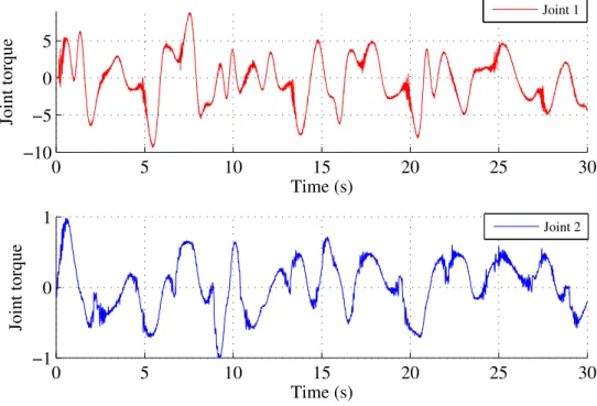
power model approach . . . 57 2.3 Comparison between IDIM-OLS and modulating function using

power model method, 2R prototype robot . . . 60 2.4 DHM configuration of 4R scara planar robot . . . 60 2.5 Comparison between IDIM-OLS and modulating functions

iden-tification approaches . . . 63 3.1 Influence of design parameters onD_{κ,µ,T ,q}(n) x(t0−T ξκ,µ,q(n) ) in

contin-uous case. . . 72 3.2 Influence of design parameters onD(_κ,µ,h,qn) x(t0) in continuous case. 79

3.3 Comparison of experimental identification with 2R prototype robot, IDIM-OLS . . . 91 3.4 Results with identification model using motor and load positions 97 3.5 Results with identification model using motor position and torque 97 3.6 Identified parameters with identification model using motor

po-sition and torque . . . 99 4.1 Different identification approaches . . . 103 4.2 Filtering systematic error of central difference with Butterworth

filter . . . 108 4.3 Filtering systematic error of central Jacobi differentiator . . . . 109 4.4 Results with IDIM-OLS, 2R prototype robot . . . 112 4.5 Results with IDIM-WLS, 2R prototype robot . . . 112 4.6 Results with power identification model, OLS, 2R prototype robot 113 4.7 Results with energy identification model method, OLS, 2R

pro-totype robot . . . 113 xxiii

4.8 Results with modulating function using power model method, OLS, 2R prototype robot . . . 114 4.9 Results with modulating function using power model method,

List of Figures

1 Diagramme de Bode du filtre FIR correspondant à la dérivation

d’ordre 2 par fonctions modulatrices avecℓ = 10 . . . . 4

2 Comparaison des réponses fréquentielles du différentiateur causal de Jacobi et des filtres classiques . . . 8

3 2R scara planar prototype robot (Lab IRCCyN) . . . 9

4 Erreurs systématiques . . . 10

5 Comparaison . . . 12

6 Development of robots . . . 14

1.1 DHM frame of 2R scara planar robot . . . 23

1.2 2R scara planar prototype robot (Lab IRCCyN) . . . 26

1.3 SYMORO+ software . . . 29

1.4 DIDIM identification scheme . . . 39

2.1 Bode plot of second order derivatives of modulating functions whenℓ = 10 . . . . 47

2.2 Estimation whenq is of SNR= 30dB, with ℓ = 2+₁₀₀i , i = 1, 2, ..., 1800

and T=4s . . . 50

2.3 Zoomed estimation whenq is of SNR= 30dB, with ℓ = 2+₁₀₀i , i = 1, 2, ..., 1800 and T=4s . . . . 51

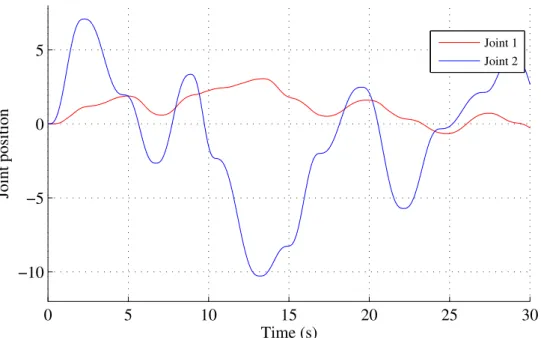
2.4 Measured joint position of 2R prototype scara planar robot . . 58

2.5 Joint torque of 2R prototype scara planar robot . . . 59

2.6 Measurement with normally disturbed random noise of SNR=30dB 62 3.1 Estimated acceleration with causal Jacobi differentiators . . . . 73

3.2 Bode plot of second order causal Jacobi differentiators . . . 74

3.3 Causal Jacobi differentiator parameters influence on bode plot whenTs = 0.001s . . . . 75

3.4 Derivative errors in velocity and acceleration with central Jacobi differentiator . . . 80

3.5 Bode magnitude plot of second order central Jacobi differentia-tors . . . 80

3.6 Phase response of second order central Jacobi differentiators . 81 3.7 Central Jacobi differentiator parameters influence on bode plot whenTs = 0.001s . . . . 83

3.8 IDIM-ILIC scheme . . . 85

3.9 IDIM-ILIC identification results . . . 87

3.10 IDIM-ILIC tracking error with simulation . . . 88 xxv

3.11 IDIM-ILIC computed torque with simulation . . . 88

3.12 Estimation inZZ1R,ZZ2,LMX2,LMY2 with variation ofZZ1R 89 3.13 IDIM-ILIC tracking error with simulation and variation ofZZ1R 89 3.14 2R prototype robot trajectory and estimation of velocities, accel-eration ofq1 . . . 90

3.15 EMPS prototype system . . . 91

3.16 EMPS components . . . 92

3.17 EMPS modeling and DHM frames . . . 93

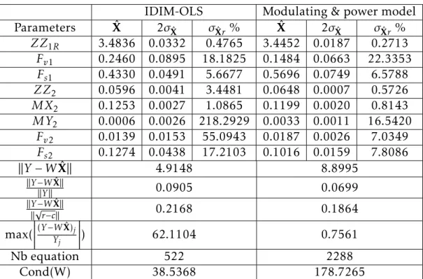
3.18 Cross validation with identification model using motor and load positions . . . 98

3.19 Cross validation with identification model using only motor po-sition and torque . . . 100

3.20 Cross validation error with two identification model . . . 101

4.1 Bode plot cutoff frequency at 8 Hz of band-pass filtering for posi-iton, velocity and acceleration . . . 107

5.1 Structure of iterative learning controller with real time estima-tion . . . 119

5.2 Reference trajectory . . . 123

5.3 Computed torque with updation of accurateM and N . . . . . 124

5.4 Computed torque in normal tracking task . . . 124

5.5 Computed torque whenZZ1R varies . . . 125

5.6 Computed torque in normal tracking task with noise . . . 125

5.7 Estimated parameters and tracking error in normal tracking task 128 5.8 Estimation ofM, N and tracking error when ZZ1R varies . . . 129

5.9 Estimation of M, N and tracking error in normal tracking task with noise . . . 130

Résumé français

Introduction

La plupart des contrôleurs avancés ont besoin d’une bonne connaissance du modèle dynamique du robot pour leur mise en œuvre. Le modèle dynamique du robot peut être développé selon la méthode de Newton-Euler ou la méthode de Lagrange. Il décrit la dynamique du système en termes de position, vitesse, l’accélération et force ou couple, ainsi que des paramètres dynamiques. Les paramètres dynamiques sont des constantes comme la masse, l’inertie, les mo-ments d’inertie, les paramètres de frottement de chaque articulation du robot, et le moment d’inertie global des éléments composant la chaîne cinématique du réducteur. Puisque les paramètres dynamiques sont inconnus, ils doivent d’être identifiés avant l’opération. De nombreux paramètres ne sont pas mesurables directement et doivent donc être identifiées à partir de mesures sur le robot en fonctionnement. Donc, la procédure d’identification des paramètres dy-namiques est nécessaire. Dans la littérature, plusieurs méthodes ont été pro-posées pour résoudre ce problème, basée sur l’utilisation les 3 modèles:

• modèle dynamique (Canudas de Wit et al., 1991; Gautier, 1986; Gautier et al., 2008, 2013; Gautier and Khalil, 1990; Gautier, Khalil, and Restrepo, 1995; Gautier, Vandanjon, et al., 2011; Hollerbach et al., 2008; Khalil and Dombre, 2004; Khosla et al., 1985; Lu et al., 1993);

• modèle d’énergie (Gautier, 1996; Gautier and Khalil, 1988); • modèle de puissance (Gautier, 1997).

L’objectif de cette thèse est de développer de nouvelles techniques en iden-tification des paramètres dynamiques des robots et de les comparer avec les techniques existantes. Nous proposons de nouvelles techniques sur deux as-pects: reformuler le modèle du robot en utilisant les fonctions modulatrices; appliquer les différentiateurs de Jacobi développés récemment pour résoudre le

problème de dérivation et analyser leur propriétés de filtrage dans le domaine fréquentiel.

Fonctions modulatrices en identification

Soitl∈ N∗,T ∈ R∗+, etg une fonction satisfaisant des propriétés suivantes:

(P1) : g ∈ Cl([ta, tb]);

(P2) : g(i)(ta) =g(i)(tb) = 0, pour i = 0, 1, ..., l− 1; (1) avec_Cl([ta, tb]) l’ensemble des fonctions qui sontl−fois continûment dérivable sur la fenêtre de temps [ta, tb] avec l ∈ N∗. La fonction g définit une fonction modulatrice d’ordre l sur [t_a, tb].

Les fonctions modulatrices peuvent être utilisées pour l’identification. Sup-posons quex(d) est d’ordre d, avec x la variable d’observation et s est un

nom-bre entier. On peut faire diminuer l’ordre de la dérivéex(d) grâce aux fonctions modulatrices. Par exemple, soit g une fonction modulatrice d’ordre l définie

sur l’intervalle [0, T ], avec l ≥ d. On multiplie g par x(d) et on intègre par partie le produit g sur la fenêtre de temps [0, T ]. Ce qui permette les dérivées de x

vers les dérivées deg, qui sont analytiquement connues.

∫ T 0 gx(d)=− ∫ T 0 ˙gx(d−1)=··· = (−1)d ∫ T 0 g(d)x. (2)

Analyse dans le domaine fréquentiel

Les intégrales (2) sont des intégrales de convolution correspondant à un filtrage qui peut être analysé dans le domaine fréquentiel.

Dans (Chen et al., 2011; Collado et al., 2009), les auteurs analysent égale-ment la propriété de différenciation dans le domaine fréquentiel. Le calcul pratique de ∫ gx se fait sous la forme d’une convolution numérique avec une période d’échantillonnage Ts, et conduit à une version discrète sous la forme

∑N

i=1g[i]x[i]. De cette façon, la convolution avec les fonctions modulatrices peut être analysée comme un filtre à réponse impulsionnelle finie (FIR) dont les coefficients sont les valeursg(t).

Les fonctions proposées gℓ(t) sont des fonctions modulatrices d’ordre K sur l’intervalle [0, T ], avec K l’ordre maximum de dérivation de x à calcule. Les

fonctionsg(t) satisfont les deux conditions aux limites: g_ℓ(i)(0) = 0, etg_ℓ(i)(T ) = 0,

quandi = 0, 1, . . . , K− 1.

(1) Les fonctions modulatrices sinusoïdales (SMF): la valeur de la fonction sinusoïdale atteint 0 à chaque demi-période, et on proposegℓ(t) = sinℓ(_Tπt), avec

ℓ∈ R.

(2) Les fonctions modulatrices de Jacobi (JMF): ce groupe de fonctions est une combinaison de polynômes de Jacobi qui vaut 0 au début et à la fin de l’intervalle [0, T ]. Il faut faire attention à ce que l’ordre des fonctions

modula-trices soit supérieur àK− 1 et on propose gℓ(t) = tℓ1_{(t− T )}ℓ2_{, avecℓ}

1, ℓ2 ∈ R et

ℓ1, ℓ2> K− 1.

(3) Les fonctions modulatrices de Fourier (FMF): la fonction exponentielle

eix = cosx + i sin x est une fonction périodique qui atteint 1 à chaque période.

Grâce à cette propriété, on peut écrire les fonctions modulatrices de Fourier sous la formegℓ(t) = e−iαℓ(e−i

2π

T t− 1)K, oùα est paramètre de réglage et ℓ∈ R.

(4) Les fonctions modulatrices de Harley (HMF): elles sont basées la méth-ode de Shinbrot et Pearson Fourier fonctions modulatrices, ce groupe de fonc-tions est donné par :

gℓ(t) =∑nj=0(−1)j       n j     

cas((n + ℓ− j)ω0t), où ℓ = 0,±1,±2,... est entier, ω0 =

2π T est la résolution fréquentielle et cas(x) = cos x + sin x.

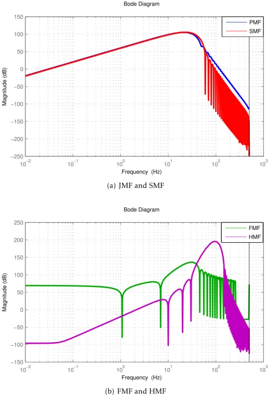
Les 4 types de fonctions modulatrices sont analysées d’un point de vue fil-trage en calculant la forme discrète de la convolution dans laquelle les valeurs degℓ(t)ĺéchantillonnée à la période de Ts, sont les coefficients d’un FIR. Par ex-emple, les diagramme de Bode en amplitude Fig. (1) représentent la réponse fréquentielle de FIR définie pour le calcul de la dérivée seconde avec les 4 types de fonctions modulatrices.

Identification en utilisant les fonctions modulatrices et le

mod-èle de puissance

Les fonctions modulatrices peuvent être appliquées à l’identification des paramètres dynamiques des robots, sous la forme d’une convolution avec le modèle de puissance du robot. Rappelons le modèle de puissance (3) d’un robot avec n

articulations:

˙qTΓ_m= d

dt(H) + ˙q

T_{[diag( ˙q)F}

v+diag(sign( ˙q)Fs+ Γoff]. (3)

oùq, ˙q sont des vecteurs de la position et de la vitesse, de dimension (n × 1), Γm est le couple de moteur,H est l’énergie totale du robot, H(q, ˙q) = E(q, ˙q + U(q)

est la somme de l’énergie cinétique de l’articulationE et de l’énergie potentielle U. H et linéaire par rapport aux parametres inertials K de robot. H(q, ˙q) =

10−2 10−1 100 101 102 103 −250 −200 −150 −100 −50 0 50 100 150 Magnitude (dB) Bode Diagram Frequency (Hz) PMF SMF (a) JMF and SMF 10−2 10−1 100 101 102 103 −150 −100 −50 0 50 100 150 200 250 Magnitude (dB) Bode Diagram Frequency (Hz) FMF HMF (b) FMF and HMF

Figure 1 – Diagramme de Bode du filtre FIR correspondant à la dérivation d’ordre 2 par fonctions modulatrices avecℓ = 10

h(q, ˙q)K, les coefficients de h définissent les fonctions d’énergie. F_vj,Fsj sont les coefficients de frottement visqueux et de Coulomb de l’articulationj, Γof f j est un paramètre d’offset (Gautier et al., 2013).

On intègre par partie, l’équation (3) pondérée par des fonctions modulatri-ces de premier ordreg sur l’intervalle [ta, tb] et :

∫ t_b ta g ˙qTΓ_{mdt =−} ∫ t_b ta ˙ghKdt + ∫ t_b ta g ˙qTdiag( ˙q)Fvdt + ∫ t_b ta tg ˙qTdiag(sign( ˙q))Fsdt + ∫ t_b ta g ˙qTΓ_{offdt. (4)} Cette équation scalaire correspond aux modèle d’énergie pondéré parg, ce

qui évite le calcul numérique de la dérivée d’ordre 2.

connaissons l’expression analytique de l’énergieh et les dérivées des fonctions modulatrices. En calculant (4) par différentes fonctions modulatricesgℓ.

On obtient un système linéaire surdéterminé den× nt× nméquations:

Y_E=W_E(q, ˙q, ¨q)X + ρ_E, (5)

oùnt est le nombre d’intervalles de temps,nm est le nombre de fonctions mod-ulatrices,ρE est le bruit, YE etWE sont respectivement le vecteur et la matrice

d’observation, qui sont définis comme:

Y_E=                         tb1 ∫ ta1 g1q˙TΓm ... t_bnt ∫ t_ant gneq˙ TΓ_m                         , WE=                         − tb1 ∫ ta1 ˙g1h(q, ˙q) ... − t_bnt ∫ t_ant ˙gneh(q, ˙q)                         . (6)

Le système (5) est résolu en utilisant des techniques de moindres carrés.

Differentiateur de Jacobi

Les différentiateurs numériques introduits dans cette partie sont basés sur des méthodes algébriques. Ils sont d’abord proposés par Fliess et Sira-Ramírez dans un article récent (Fliess, Mboup, et al., 2003; Fliess and Sira-Ramirez, 2004). Ces différentiateurs algébriques sont divisés en deux classes: les différentia-teurs basés sur des modèles et les différentiadifférentia-teurs sans modèle. Les premiers (Fliess and Sira-Ramrez, 2004; Tian et al., 2008). ont été principalement utilisés pour les systèmes linéaires. Ils ont été étendus aux différentiateurs sans modèle, qui peuvent être utilisés pour les systèmes non linéaires et divers problèmes en traitement du signal. Le premier facteur de différentiation sans modèle a été introduit dans (Fliess, Join, et al., 2004) en appliquant la méthode algébrique de développement tronqué en série de Taylor du signal à différentier. Puis, deux différentiateurs sans modèle ont été étudiés dans (Mboup et al., 2007, 2009a). En outre, il a été montré que le différentiateur causal peut également être obtenu en projetant le signal sur la base orthogonale de Jacobi. Ensuite, il a été significativement amélioré en admettant un retard choisi par le concepteur (Mboup et al., 2007, 2009a). Dans (Liu et al., 2011c), un différenciateur central de Jacobi a été proposé, pour une utilisation hors ligne.

par une intégrale définie sur une fenêtre glissante dans le cas continu, leur comportement de filtre passe-bande et correspond à une convolution dans le cas discrèt. En outre, le caractère passe-bande dans les hautes fréquences qui est robuste par rapport aux bruits (Fliess, 2006). Une étude théorique démon-tre que les erreurs sont des fonctions fortement non linéaires des paramèdémon-tres de conception et que les erreurs sont limitées. D’autre part, quelques travaux expérimentaux montrent la relation entre les erreurs et les paramètres de con-ception (Liu et al., 2009a, 2011a, 2012a). Cependant, il n’existe pas encore de méthode efficace de conception en différentiateur de Jacobi, car les paramètres sont fortement couplés. Pour résoudre ce problème, j’ai proposé une écriture du différentiateur Jacobi sous la forme d’un FIR, ce qui permet d’analyser son comportement fréquentiel et fournit un outil de conception.

On présente ici les différentiateurs causaux de Jacobi, utilisés aussi pour les différentiateurs centrales de Jacobi. Soit une mesure bruitéexϖ:I → R, xϖ(t) = x(t) + ϖ(t), où I est un interval ouvert de temps fini R+, x ∈ Cn(I) avec n ∈ N, etϖ est un bruit. L’objectif est d’estimer la dérivée d’ordre n de x en utilisant xϖ. On applique les polynômes de Jacobi pour calculer le développement série orthogonale pour estimer lanièmedérivée, (Mboup et al., 2007, 2009a).

D’abord, pour toutt0∈ I, on introduit Dt0 :={t ∈ R∗+;t0− t ∈ I}. La définition

du polynôme d’ordre i décalé sur l’intervalle [0, 1] est (voir dans(Abramowitz

et al., 1965) pp. 774-775), oùµ, κ∈] − 1,+∞[: P_i(µ,κ)(τ) = i ∑ j=0 (i + µ j )(i + κ i− j ) (τ− 1)i−jτj. (7)

Définissons sur _L2([0, 1]) un produit scalaire ⟨·,·⟩(0µ,κ,1) avec la fonction de poids ˆwµ,κ(τ) = (1− τ)µτκ, notons∀g1, g2∈ C[0,1], ⟨g₁, g2⟩(0µ,κ,1)= ∫ 1 0 ˆ wµ,κ(τ)g1(τ)g2(τ)dτ. (8)

Et la norme associée au polynôme orthogonaux décalé de Jacobi d’ordre i est

donnée par: _∥Pi(µ,κ)_∥2_µ,κ =_2i+µ+κ+11 ΓΓ(₍µ+i+1)Γ(κ+i+1)_{µ+κ+i+1)Γ(i+1)}, où Γ(n) est la fonction Gamma

(voir (Abramowitz et al., 1965) p. 255), avec Γ(n) = (n− 1)!.

Le calcu sous la forme d’un différentiateur causal de Jacobi est présenté en détail dans (Liu et al., 2012a). Ici, nous donnons l’expression continue analy-tique du différentiateur causal de Jacobi, qui calcule lanième dérivée à l’instant

t₀,∀ξ ∈ [0,1],∀t0∈ I, D_{κ,µ,T ,q}(n) x(t0− T ξ) = 1 (−T )n ∫ 1 0 Qκ,µ,n,q,ξ(τ) x(t0− T τ)dτ, (9) avecµ, κ∈] − 1,+∞[, Cκ,µ,n,i = (µ + κ + 2n + 2i + 1)Γ(κ + µ + 2n + i + 1)Γ(n + i + 1) Γ_{(κ + n + i + 1)Γ(µ + n + i + 1)} , (10) Qκ,µ,n,q,ξ(τ) = ˆwµ,κ(τ) q ∑ i=0 Cκ,µ,n,iP (µ+n,κ+n) i (ξ)P (µ,κ) n+i (τ). (11)

Enfin, nous remplaçons x dans (9) par xϖ pour obtenir D_{κ,µ,T ,q}(n) xϖ(t0− T ξ)

dans le cas bruité.

L’idée de ce différentiateur est d’utiliser une fenêtre d’intégration glissante pour estimer la valeur dex(n) pour chaque t0 ∈ I par Dκ,µ,T ,q(n) x(t0− T ξ) avec la

valeur fixéeξ ∈ [0,1], l’optimisation de ξ est donnée dans ((Mboup et al., 2007, 2009a)). Siξ , 0, alors on a un retard de T ξ.

Il dépend d’un ensemble de paramètres:

•κ, µ∈] − 1,+∞[: les paramètres du polynômes de Jacobi,

•q∈ N: l’ordre du développement de la série Jacobi tronqué,

•T ∈ Dt0: la longueur de la fenêtre glissante d’intégration,

•ξ ∈ [0,1]: le paramètre de retard T ξ.

L’analyse fréquentielle permet de caractériser le comportement du différen-tiateurs de Jacobi dans Fig. (2). On compare à un filtre FIR et à un filtre passe-bande composé d’un filtre passe-bas de Butterworth, suivi d’une dérivée par différence. Les résultats montrent que le différentiateur causal de Jacobi présente une phase linéaire au voisinage de la fréquence de coupure avec une propriété de filtrage passe bas en hautes fréquences intéressantes.

Comparaisons des méthodes d’identificaiton des paramètres

dynamiques des robot

Dans le tableau (1), on rappelle les différentes techniques d’identification en robotique.

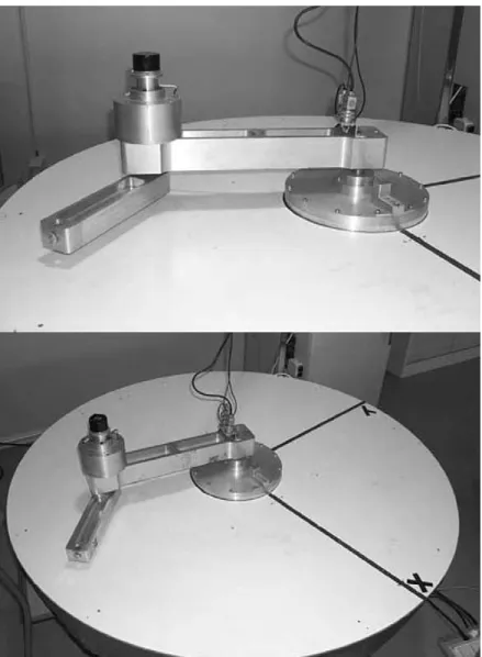
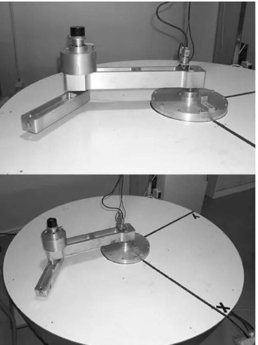
Une étude comparative des méthodes d’identification est réalisée sur un prototype de robot SCARA sans gravité à deux articulation à entraînement di-rect développé au laboratoire (IRCCyN) (Presse, 1994) comme indiqué sur Fig.

10−1 100 101 102 103 −100 −50 0 50 100 150 200 Magnitude (dB) Bode Diagram Frequency (Hz) FIR+Difference BW+Difference Causal Jacobi Ideal (a) Amplitude 5 10 15 20 25 30 35 40 −135 −90 −45 0 45 90 135 180 Phase (deg) Bode Diagram Frequency (Hz) FIR+Difference BW+Difference Causal Jacobi Ideal (b) phase response

Figure 2 – Comparaison des réponses fréquentielles du différentiateur causal de Jacobi et des filtres classiques

(3). Le modèle dynamique dépend de 4 paramètres inertiels minimaux, et de 4 paramètres de frottement:

X = [ZZ1R, ZZ2, LMX2, LMY2, Fv1, Fs1, Fv2, Fs2], (12) avecZZ₁R=ZZ1+M2L2.

Résultats d’identification

Pour étudier les erreurs systématiques dues à la distorsion des différentes filtres, on simule le modèle du robot sans bruit avec la valeurs deX en unités SI : X = [3.5 0.06 0.15 0.1 0.3 0.4 0.2 0.12]. Les résultats sont présentés dans la Fig. (4).

Modèle d’identification Différentiateurs Moindre carré

Modèle dynamique (IDIM) différence & Butterworth OLS1

Modèle de puissance différentiateurs centrale de Jacobi WLS2

Modèle d’énergie Modèle de puissance avec

fonctions modulatrices

Table 1 – méthodes pour l’identification des paramètres dynamiques des robots

|XiXi− ˆXi|. Les résultats montrent que la méthode avec le différentiateur centré de Jacobi a moins d’erreurs systématiques plus faibles que les autres. D’autre part, le modèle de puissance avec les fonctions modulatrices a le résultat le plus proche des valeurs réelles. Ensuite, on réalise des essais d’identification

Figure 4 – Erreurs systématiques

sur le prototype du robot scara. Les résultats sont indiqués dans la Fig. (5). L’identification expérimentale montre :

modèle de puissance avec fonctions modulatrices = IDIM-WLS _{≥ modèle de}

puissance_{≥ modèle d’énergie ≥ IDIM-OLS .}

Conclusion

Ce travail concerne l’identification des paramètres dynamiques des robots. Les contributions suivantes ont été réalisées:

• Proposition d’unmodèle de puissance avec fonctions modulatrices qui évite la dérivation numérique des fonctions d’énergie.

• Analyser dans le domaine fréquentiel des fonctions modulatrices, qui a permis de sélectionner les fonctions modulatrices de filtre passe-bande adapté à l’identification.

• introduction lesdifférentiateurs de Jacobi et analyser pour la première fois, dans le domaine fréquentiel pour qualifier et quantifier leurs pro-priétés de filtrage. La majeur de la thèse a permis de comparer les differ-entiateurs de Jacobi en terme de distorsion et d’établissement des bruits hautes fréquences.

• comparaison entre les modèles différents d’identification, dynamic, de puissance d’énergie, des différentiateurs, des techniques de moindre carré pour l’identification des robots.

Un problème important dans l’identification des paramètres dynamiques des robots est de diminuer au maximum l’influence du bruit dans la dériva-tion des signaux. Dans ce travail, nous proposons des méthodes basées sur des techniques algébriques: utiliser le modèle de puissance avec les fonctions mod-ulatrices ce qui supprime le calcul de l’accélération et le calcul de la dérivée des fonctions d’énergie; appliquer les différentiateurs de Jacobi pour obtenir une bonne estimation des dérivées d’ordre 2.

Les travaux futurs concernent une validation sur des robots plus complexes, qui ont un comportement non-linéaire accentué avec un grand nombre de paramètres, ce qui entraîne des difficultés pour l’identification.

(a) Moyennes de l’écart type relatif (%)

(b) Résidus norme relative maximale max(      (Y−W ˆX)j Yj      )

(c) Résidus norme relative

(d) Conditionnement Figure 5 – Comparaison

General Introduction

A robot is a mechanical or virtual artificial agent, usually an electro mechanical machine that is guided by a computer program or electronic circuitry. As a word, robot is drawn from an old Church Slavonic word, robota, for "servitude," "forced labor" or "drudgery." The word, which also has cognates in German, Russian, Polish and Czech, was a product of the central European system of serfdom by which a tenants rent was paid for in forced labor or service.

The first robot can be tracked back to the 4th century BC, when a wooden, mechanical steam-operated bird called The Pigeon was created by the Greek mathematician Archytas. While the research into the functionality and po-tential uses of robots did not grow substantially until the 20th century. Es-pecially, fully autonomous robots only appeared in the second half of the 20th century and the robotics subject keeps prosperity and development. More re-cently, "robots" and the derived term "robotics" have come to represent the most modern engineering technologies for a myriad of functions ranging from artifi-cial intelligence experiments and building automobiles to performing delicate surgical procedures.

Robotics are crossing disciplines of mechanical engineering, electrical engi-neering and computer science that deals with the design, construction, opera-tion and applicaopera-tion of robots, as well as the computer systems for their control, sensory feedback and information processing.

With the fast development of robot theory, people gradually became aware of the geometry and dynamic descriptions of the robot, with better and better precision in building mathematical model. Consequently, most of the advanced robot control schemes are proposed with application of the robot model, espe-cially the robot dynamic models, in order to adjust the controller and the in-crease the control precision. Such control schemes include: computed torque control; predictive control; passivity control; adaptive control.

It requires a good knowledge of the robot dynamic model before implemen-tation. Robot dynamic model can be developed from Newton-Euler method or Lagrange method. It describes the system dynamics in terms of current states,

Ancien Modern Future

Figure 6 – Development of robots

such as position, velocity, acceleration and force/torque, as well the dynamic parameters. The dynamic parameters are constant at each instant and include the mass, inertia, first moments, joint friction for each robot link, and moment of inertia of the rotor and transmission system of actuators. As the key elements of the robot model, they need to be recognized before operation. However, for some of them, it is not likely to implement a measurement by the existing tech-nology. Thus, the identification procedure is necessary and as a long-standing subject in the robotics.

In this work, we investigate the robot identification issue. The aim is to identify robot’s dynamic parameters via a measurement of robot trajectory and torque/force information. Various identification methods have been developed based on different robot models, differentiation approaches, numerical tools, sensor feedback information or cross validation using closed loop simulation. Illustrating results are obtained in the past decades, while there still exist some challenges in the differentiation problem. In robot applications, the obtained measurements are usually noisy, which makes the derivative estimation process be ill-posed in the sense that a small error in measurement can induce a large error in the computed derivatives, specially for high order derivatives. The poor performance of reconstructing derivatives from the noisy measurement will directly induce some bias in the identification matrix, which results in huge errors in the identification results. Moreover, the highly nonlinear property of the robot systems and its large number of dynamic parameters also bring in difficulty in identification. Therefore, more researches and studies should be

carried out in this area.

The Project-team Non-A has developed a group ofalgebraic differentiators, called Jacobi differentiators. They provide the solution as an explicit integral formulae associated with finite signal information within a sliding integration time window. Because of their integration structure, they behave as nature filtering process and are robust to corrupt noises. Compared to other differ-entiators, Jacobi differentiators can be implemented immediately without pre-filtering of the noisy signal due to their integral structure.

Meanwhile based on the algebraic conception, it is possible to transform the high order differential equation into lower order one. Associated with the mod-ulating functions, the differential equation is rewritten in a simple expression which could eliminate certain high order terms by using some annihilating in-tegral operator. The robot identification model can also apply this technique in order to avoid the terms with joint acceleration, which is usually badly esti-mated.

Objective of the thesis

The main objective of this thesis is to develop new techniques in robot dynamic parameters identification methods and compare them with the existing tech-niques. We propose new approaches in two aspects : reformulate the robot model using both the algebraic method and modulating functions; apply the newly developed Jacobi differentiators in robot differentiation problem and analyse the filtering property in frequency domain. In the end, we discuss if the detailed identification model is needed for control and based on the alge-braic method, a simple and fast response adaptive controller is designed.

Outline of the thesis

Chapter 1 gives an overview of the existing approaches for serial robot identi-fication process. The principle of theidentification procedure is based on the analysis of the ’input/output’ behavior of the robot following some planned motion and on estimating the parameters value by minimizing the difference between a function of the real robot variables and its mathematical model. Ac-cording to the models, the most widely applied approach is based onrobot ex-plicit dynamic model, requiring the joint force/torque, position, velocity and acceleration information. The other models such as robot energy model and

robot power model require only the joint force/torque, position and velocity information. However they need an additional derivative operation on the im-plicit expression of velocity. As the dynamic parameters are linear with respect to the models above, most of the identification processes form an overdeter-mined system by a sequence of measurements and obtain the optimal solution using the least-square techniques. Besides, a parallel scheme to identify robot dynamic parameters by minimizing the output error from a closed loop simu-lation is presented.

Chapter 2 investigates the new identification method. It starts from an alge-braic point of view, by which the order of differential equation can decrease us-ing some annihilatus-ing operator. Based on this technique, the robot power model is transformed to an energy equation, that does not consider the acceleration variables and the implicit derivative operation. In this sense, the identification model avoids using the inaccurate acceleration information and introduce less errors in the results. Meanwhile, the modulating functions are implemented during the process. We will analyse their magnitude-frequency response and show that they have a low-pass filtering property for certain groups of the modulating functions.

Chapter 3 discusses the differentiation problem in robot identification is-sues. The principle and analysis of the causal and central Jacobi differentia-tors are introduced. As well, their frequency domain properties are analysed via a finite impulse response (FIR) filter point of view, indicating clearly their differentiation performance. Comparisons with other differentiators are made both in time domain and frequency domain.

Chapter 4 presents mainly the identification results in simulation and ap-plication of different approaches, in order to give a clear understanding of the advantages and draw-backs for each methodology. To be more specific, four different identification models (dynamic, power, energy identification models, modulating functions with power model approach), two differentiators (Jacobi differentiators and central difference with Butterworth filter) and three least square techniques (Ordinary, Weighted, Iterative least squares techniques) are compared.

Chapter 5 studies from the control aspect, some new ultra local robot model, which represents well the robot dynamics. Here "ultra local" means on a small time window. An adaptive controller is proposed so that by estimating the states of the simplified model, the corrupt changes of the robot are detected and updated within a short time window, which offers better dynamic perfor-mance of the control scheme. Moreover, the estimation model jumps over the

traditional differentiation problem in robotics, and only needs the joint force/-torque and position information. In the 2-DOF (degrees of freedom) planar robot simulation test, the estimation window is reduced to 0.1 second in

pres-ence of noise.

Chapter

1

Overview of the robot identification

problem

Accurate dynamic models of robots are required in most advanced control schemes formulated in recent literature (Khatib, 1987; Piltan et al., 2012; Slotine et al., 1987). The precision, performance, stability and robustness of these schemes depend on, to a large extent, the accuracy of the dynamic parameters. Adap-tive and robust control scheme can tolerate some error in the dynamic param-eters, while other schemes designed to achieve perfect feedback linearization, such as computed torque control, assuming precise knowledge of the dynamic parameters. In this sense, the precise determination of the dynamic parame-ters is useful to most schemes and is crucial to some others. Furthermore, the dynamic parameters are necessary to simulate the robot dynamics.

However, accurate values of the dynamic parameters are typically unknown, even to the robot manufactures, and the measurement for some of them are practically not accessible. Thus, the indirect identification approaches are considered through the analysis of the ’input/output’ behavior of the robot fol-lowing some planned motion and on estimating the parameters value by min-imizing the difference between a function of the real robot variables and its mathematical model. The identification problem turns out to be an optimiza-tion quesoptimiza-tion which searches for the correct robot model with proper dynamic parameters.

The following parts present the principle of identification procedures and the related various techniques. According to the inputs that the identification model needs, there exists threerobot identification models:

• robot dynamic model (Canudas de Wit et al., 1991; Gautier, 1986; Gau-tier et al., 2008, 2013; GauGau-tier and Khalil, 1990; GauGau-tier, Khalil, and

strepo, 1995; Gautier, Vandanjon, et al., 2011; Hollerbach et al., 2008; Khalil and Dombre, 2004; Khosla et al., 1985; Lu et al., 1993);

• robot energy model (Gautier, 1996; Gautier and Khalil, 1988); • robot power model (Gautier, 1997).

The robot dynamic model is the most widely implemented identification model. It establishes the dynamic equations at individual point along the tra-jectory. The advantages of this model include that it is easy to create the dy-namic equations and it has a good excitation in the identification regression matrix, which means the regression always has a solution. By contrast, the dy-namic model contains the acceleration variables, which are usually inaccurate computation using the position measurement. While the robot energy model and power model avoid using the acceleration data. Instead, the energy model applies an integral operation on the robot power equation and the power model make use of the differential equation of the energy part. In the following, we will present these identification process. Note that for the rest part of the thesis, we denote the bold mathematical symbols for the vectors or matrix.

1.1 Inverse dynamic identification model with LS

Γ_{m as a function of the state variables and their derivatives. It can be deduced} from the followingLagrangian formulation:

Γ_m= d dt ( ∂L ∂ ˙q ) −∂L_∂q+ Γ_f, (1.1)

where_{q, ˙q are the (n × 1) vectors of generalized joint positions and velocities, L} is the Lagrangian of the system defined as the difference between the kinetic energy E(q, ˙q) and the potential energy U(q). E = 1₂˙qTM(q) ˙q, where M(q) is the (n× n) robot inertia matrix. Γf is the friction torque which is usually

mod-elled at non zero velocity as Γ_{f j} = Fsjsign( ˙qj) +Fvj˙qj + Γof f j, where ˙qj is the velocity of jointj, sign(x) denotes the sign function. Fvj,Fsj are the viscous and Coulomb friction coefficients of jointj, Γof f j is an offset parameter which is the dis-symmetry of the Coulomb friction with respect to the sign of the velocity

and is due to the current amplifier offset which supplies the motor (Gautier et al., 2013).

Develop Eq. (1.1) by replacing L with E− U, and it becomes the inverse dynamic model:

Γ_{m=M(q) ¨q + C(q, ˙q) ˙q + Q(q) + Γf, (1.2)}

where ¨q is the n × 1 vector of joint acceleration, M(q) is the n × n symmetric and positive definite inertia matrix, _{C(q, ˙q) ˙q is the n × 1 vector of Coriolis and} centrifugal torques,_{Q(q) is the n × 1 vector of gravity torques.}

The inverse dynamic model is linear with respect to a set of standard dy-namic parameters Xs, because E, U and Γf are linear with respect to the

dy-namic parameters (Gautier, 1990). Thus, the model (1.2) can be rewritten as:

Γ_{m=Ds(q, ˙q, ¨q)Xs=} Ns

∑

i=1

DsiXsi, (1.3)

whereNsis the total number of the dynamic standard parameters,Dsis an×Ns

matrix, andDsi is the ith column of Ds, Xsi is the ith element of Xs. Xs is the vector of standard dynamic parameters:

Xs= [ X1_sT X2_sT ··· XnsT ] , withXjs T

is the dynamic parameters of joint and linkj:

Xjs= [XXj XYj XZjY Yj Y Zj ZZj MXj MYj MZj Mj IAjFvj Fsj Γof f j]T, whereXXj XYj XZj Y Yj Y Zj ZZj are the six components of the inertia matrix of link j; MXj MYj MZj are the three components of the first moments; Mj is the mass of link j, IAj is the total inertia moment for rotor actuator and gears of actuatorj; Fvj, Fsj, Γof f j are the viscous, Coulomb and offset friction parameters of jointj.

According to (Gautier and Khalil, 1990; Mayeda et al., 1990), the set of standard dynamic parameters can be simplified into a set of base inertial pa-rameters, which are the minimum parameters that can be used to describe the robot dynamics. These base parameters are obtained from the standard inertial dynamic parameters by eliminating those that have no effect on the dynamic model and by regrouping those in linear relations. In (Gautier, 1991), symbolic and numerical solutions are presented for any open or closed chain robot

ma-nipulator to get a minimal dynamic model:

Γ_{m=D(q, ˙q, ¨q)X, (1.4)}

whereX is the N_{b× 1 vector of base parameters.}

1.1.1 Case study: the 2R scara planar prototype robot of

IRC-CyN

To illustrate the construction of robot dynamic model, here we present a two joint scara planar robot, called 2R robot for short. As shown in Fig. 1.1, the robot geometry is described in table (1.1) using the modified Denavit and Harten-berg notation (DHM) method, with

• j denotes the jth joint,

• σ_j denotes the type of joint, 0 for revolute joint, 1 for prismatic joint, • αj is the angle betweenzj−1andzjaboutxj−1,

• dj is the distance betweenzj−1andzjalongxj−1,

• θj is the angle betweenxj−1andxj aboutzj, • rjis the distance betweenxj−1andxj alongzj,

• q1andq2 are joint position for joint 1 and joint 2 respectively,

• L is the length of the first robot link, L2 is the length of the second robot

link.

j σ α d θ r

0 0 0 0 q₁ 0

1 0 0 L q2 0

Table 1.1 – Modified Denavit and Hartenberg notation presentation of 2R scara planar robot

Before regrouped into base parameters, there exist 11 standard inertia pa-rameters for each joint, such as in table (1.2):

Notice the special geometric configuration and apply the regrouping rule (Gautier, 1990) on the 2R robot, and it can be concluded as:

0 o

o

x

x

y

y

y

x

q

q

z

z

z

o

L

L

(a) 2R scara planar robot

(b) Frame and joint variables

XXj XYj XZj Y Yj Y Zj ZZj MXj MYj MZj Mj IAj Table 1.2 – Standard inertia parameters of 2R scara planar robot

• joint 1 and joint 2 are direct drive so that the link 1 and 2 are attached to the rotors of motor 1 and 2. Then, the inertia momentZZ1 andZZ2 are

the inertia moment of links plus the inertia moment of rotorsIA1andIA2

respectively, so that in the followingIAj= 0;

• joint 2 is revolute: Y Y2,MZ2, M2 can be regrouped with other dynamic

parameters of link 2 and 1;

• the axe of joint 2 is parallel to that of joint 1 :XX₂,XY₂,XZ₂,Y Z₂can be eliminated;

• joint 1 is revolute, and the axe is along the gravity direction: only the inertia parameterZZ1 is considered;

• for joint 1, ZZ1 is grouped withM2 using the following relationZZ1R =

ZZ1+M2L2.

It is shown in table 1.3 that there exist five base inertia parameters for 2R scara planar robot.

j XXj XYj XZj Y Yj Y Zj ZZj MXj MYj MZj Mj IAj

1 0 0 0 0 0 ZZ1R 0 0 0 0 0

2 0 0 0 0 0 ZZ2 MX2 MY2 0 0 0

Table 1.3 – Base parameters of 2R direct drive scara planar robot

In order to compute the Lagrangian formulation, we need to calculate the kinetic energyE(q, ˙q) and the potential energy U(q). Because the robot is

mov-ing in a horizontal plan, the potential energy keeps constant, which means the

n× 1 vector of gravity torques Q(q) is null. The kinetic energy calculates from the following relation

E =1 2ZZ2( ˙q1+ ˙q2) 2₊1 2ZZ1R˙q 2 1

+LMX2˙q1cos(q2)( ˙q1+ ˙q2)− LMY2˙q1sin(q2)( ˙q1+ ˙q2). (1.5)

The symmetric (2_{× 2) inertia matrix M(q) can be deduced from the kinetic} energy

E =1

2˙q

From equation 1.5 and 1.6 we can calculate

M(1, 1) = ZZ1R+ZZ2+ 2LMX2cos(q2)− 2LMY2sin(q2),

M(1, 2) = ZZ2+LMX2cos(q2)− LMY2sin(q2),

M(2, 1) = M(1, 2),

M(2, 2) = ZZ2. (1.7)

Then×n matrix of Coriolis and centrifugal torques C(q, ˙q) comes from M(q) andE, which is given as

C(i, j) = n ∑ k=1 ci,jk˙qk, ci,jk = 1 2 [ ∂M(i,j) ∂qk +∂M(i, k) ∂qj − ∂M(j, k) ∂qi ] . (1.8)

After calculation, we have the explicit form

C(1, 1) =− ˙q2(LMY2cos(q2) +LMX2sin(q2)),

C(1, 2) =−( ˙q1+ ˙q2)(LMY2cos(q2) +LMX2sin(q2)),

C(2, 1) = ˙q1(LMY2cos(q2) +LMX2sin(q2))

C(2, 2) = 0. (1.9)

For friction, because it has two links, the friction torque can be given as Γ_{f(1) =Fv1˙q1+Fs1sign( ˙q1) + Γof f 1,}

Γ_{f(2) =Fv2˙q2+Fs2sign( ˙q2) + Γof f 2. (1.10)} In all, we have the explicit expression ofM(q), C(q, ˙q), Q(q) and Γf, which

are all elements of the robot dynamic model. Moreover, because the link length

L is unknown and it appears together with MX2 and MY2, thus we can group

it intoLMX2andLMY2, whereLMX2=L× MX2,LMY2=L× MY2. Finally, the

base dynamic parameters of the 2R scara planar robot can be presented as X2R= [ZZ1R, ZZ2, LMX2, LMY2, Fv1, Fs1, Γof f 1, Fv2, Fs2, Γof f 2], (1.11) Corresponding to the mathematical model, the experimental works are car-ried out a two joints planar direct drive prototype robot manufactured in the laboratory (IRCCyN) (Presse, 1994) as shown in Fig. (1.2), without gravity ef-fect. The description of geometry is the same as in Fig. (1.1) and table (1.1).

The robot is directly driven by two DC permanent magnet motors supplied by PWM choppers. Recall the base dynamic parameters (1.11) of the 2R scara planar robot model, while in the prototype case we assume (the effect of fric-tion offset parameter Γ_{of f} are negligible) the dynamic model depends on eight minimal dynamic parameters, including four friction parameters:

X = [ZZ1R, ZZ2, LMX2, LMY2, Fv1, Fs1, Fv2, Fs2], (1.12) withZZ1R=ZZ1+M2L2.

The robot motion is driven by a PD controller with a reference of a succes-sive point to point trajectories using the 5thorder polynomial trajectory genera-tor. The joint positionq and torque Γm are collected at a 100 Hz sampling rate, where each torque Γ_mis calculated as

Γ_{mj =GT jVT j,}

with GT j the drive chain gain which is considered as a constant in the fre-quency range of the robot dynamics. This trajectory has been calculated in order to obtain a good condition number (see in 1.1.4) of the observation ma-trix (Cond(W ) = 290).

1.1.2 IDIM-LS

The inverse dynamic identification model is based on the measured or esti-mated data of Γ_m,q, ˙q, ¨q, which are collected during robot tracking of reference trajectories.

The principle is to establish the identification model (1.4) at a sufficient number of samplesti, withi = 1, . . . , ns, satisfyingn× ns ≫ Nb, in order to get an over-determined linear system ofn× ns equations:

Y = W(q, ˙q, ¨q)X + ρ, (1.13)

whereρ is a noise, Y and W are the vector of torques and the observation matrix,

respectively, which are defined as follows:

Y =             Γ_m(1) ... Γ_m(ns)             , W =             D(1) ... D(ns)             . (1.14)

each sampling instant, we build the dynamic equivalence equation: Γ_{m=D(q, ˙q, ¨q)X, (1.15)} where Γ_m =       Γ_m1 Γ_m2     

, and Γm1, Γm2 are joint torques respectively, D(q, ˙q, ¨q) is a

n× Nbobservation matrix, which has the following expression

D(1, 1) = ¨q1, D(1, 2) = ¨q₁+ ¨q₂, D(1, 3) = (2 ¨q1+ ¨q2) cos(q2)− ˙q2( ˙q2+ 2 ˙q1) sin(q2), D(1, 4) =−(2 ¨q1+ ¨q2) sin(q2)− ˙q2( ˙q2+ 2 ˙q1) cos(q2), D(1, 5) = ˙q₁, D(1, 6) = sign( ˙q1), D(1, 7) = 0, D(1, 8) = 0, D(2, 1) = 0, D(2, 2) = ¨q1+ ¨q2, D(2, 3) = ¨q1cos(q2) + ˙q1˙q1sin(q2), D(2, 4) =− ¨q1sin(q2) + ˙q1˙q1cos(q2), D(2, 5) = 0, D(2, 6) = 0, D(2, 7) = ˙q2, D(2, 8) = sign( ˙q2). (1.16) (1.17)

1.1.3 Identifiability of the dynamic parameters

Thedynamic parameters are divided into three groups: fully identifiable, iden-tifiable in linear combinations and completely unideniden-tifiable. Consequently,

the observation matrix W corresponding to this set of dynamic parameters

could be rank deficient, with the fact that some columns ofW are linearly de-pendent with respect to whateverq, ˙q, ¨q. In order to obtain a unique solution, a set of independent identifiable parameters, calledbase dynamic parameters or minimum dynamic parameters, need to be determined. The selection of base

or minimum dynamic parameters will regroup those are linearly dependent and will eliminate those who have no effect on the dynamic model.

In (Khalil and Dombre, 2004), the authors present both the symbolic meth-ods and numerical methmeth-ods to determine the base dynamic parameters. Fur-thermore, a robotic software named SYMORO+ developed by laboratory IRC-CyN is proposed to resolve base dynamic parameters, and it has been open-source since 2014 (Khalil, Vijayalingam, et al., 2014)1 . Actually, the determi-nation of the base dynamic parameters is a prerequisite for identification pro-cedure. It should be noted that the grouped values can be directly computed from the identification model, and reconstruct the robot dynamics with these grouped parameters.

Figure 1.3 – SYMORO+ software

1.1.4 Excitation of the trajectory

The trajectory used in the identification should be carefully selected, in order to improve the least-squares estimation performance, such as convergence rate and the noise immunity. Some techniques are applied to choose the optimal trajectory, namely persistently exciting trajectory.

Persistently excitation condition (PE condition) A function ω : R+→ Rnis persistently excitating if there existT , δ₁,δ₂> 0 such that

δ₁I_n≤ ∫ t+T

t

ω(τ)Tω(τ)dτ≤ δ2In, (1.18) holds for allt≥ 0, where Inis the identity matrix of ordern.

This criterion can be applied to verify if the trajectory is well excited. As stated in (Antonelli et al., 1999; Gautier and Khalil, 1992), two schemes are usually used:

• calculation of a trajectory satisfying some optimization criteria (Gautier and Poignet, 2001; Gautier and Khalil, 1992; Presse and Gautier, 1993; Swevers, Ganseman, et al., 1997; Swevers, Verdonck, et al., 2007);

• utilization of the sequential sets of special motions, where each motion will excite certain dynamic parameters. As certain parameters are already identified with respect to the global problem, the exciting trajectory is easier to find.

Physically, finding this constraint is equivalent to finding an optimal trajec-tory that can excite most the identified parameters. Several criteria have been proposed in literature (Presse and Gautier, 1993; Siciliano et al., 2008). For ex-ample, here we minimize the condition number and maximizing the smallest singular value of the observation matrixW as in (Antonelli et al., 1999). Since the optimum trajectory will be executed on the manipulator, parameterizing the optimal trajectory is also an important step. Two most common types are the quintic polynomial trajectory (Antonelli et al., 1999) and periodic trajectory (Swevers, Verdonck, et al., 2007). The former is suitable for most of industrial manipulators which only accepts simple velocity command while the later tar-gets the open-architecture controller which allows user to program an arbitrary trajectory. Here we consider the periodic trajectory as formulated in equation 1.19, which can be parameterized as a sum of finite Fourier series:

qi(t) = qi0+ N ∑

j=1

[aijsin(jωft)− bijcos(jωft)], (1.19) ˙qi(t) = N ∑ j=1 [aijjωf cos(jωft) + bijjωf sin(jωft)], (1.20) ¨ qi(t) = N ∑ j=1

wherei denotes the ith robot joint,ωf is the fundamental frequency of the ex-citation trajectory and should not excite the un-modelled dynamics of the ma-nipulator. Then, the problem of finding the optimal trajectory becomes deter-mining the coefficients qi0, aij, bij which minimize the following cost function (Presse and Gautier, 1993):

f (qi(t)) = λ1cond(W) + λ2

1

σmin(W),

(1.22) where the scalarλ₁andλ₂represent the relative weights between the condition number of the observation matrixcond(W) and inverse of the minimum

singu-lar value _σ 1

min(W). Note that the condition number of the observation matrix

2 _is

defined as

cond(W) = σmax(W) σmin(W)

. (1.23)

The condition number measures how change in input is propagated to change in output. It has the following relation

∥∆X∥

∥X∥ ≤ con(W)

∥∆W∥

∥W∥ . (1.24)

1.1.5 Data processing for the inverse dynamic identification

model

In real application, the measurements or estimations of Γ_m, q, ˙q, ¨q are cor-rupted with noise. Thus, the matrices Y and W are perturbed and the LS so-lution leads to a bias estimation. Because the matrix W(q, ˙q, ¨q) are highly non linear, it is not possible to get the analytical expression of the bias and the vari-ance. To tackle this problem, two filtering processes should be applied:

• data filtering to decrease noise effect,

• closed loop identification for the tracking the persistently excited trajec-tories.

(q, ˙q, ¨q) must be pre-filtered by a low-pass filter Fq(s), with s the derivative operator in order to eliminate high frequency noise. Usually, ˙q, ¨q are processed

using the product sFq and s2Fq on the position respectively. In practice, this

2_{The optimization problem consists of determining the trajectory, which provides a}

process can be carried out using a central difference algorithm to obtain the time derivative. The optimal filterFq(s) should have a flat amplitude response without phase shift in the range [0 ωc], where the cutoff frequency ωc > (10×

ωdyn), with ωdyn is the bandwidth of the joint position closed loop (Gautier, 1997). Meanwhile, the torque Γ_mis perturbed by high frequency torque ripple from joint drive chain in the closed loop control. Hence, it has to be filtered. Then, Γm and D(qf_q, ˙qf_q, ¨qf_q) are both filtered and down-sampled through a

decimate filter composed of a low-pass filter Fp(s), where its cutoff frequency

ωfp is approximated by 5× ωdyn. The decimate rate nd can be calculated with

nd = ₂ω_ωc_{f p} for a FIR filter andnd = 0.8×₂ω_{ωf p}c for an IIR filter, where ωc is the control rate.

Then, the new filtered linear system is obtained:

Yfp=Wfp(qfq, ˙qfq, ¨qfq)X + ρfp. (1.25)

Finally, we solve the LS problem via: ˆX = W+

fp(qfq, ˙qfq, ¨qfq)Yfp. (1.26)

1.1.6 Resolution of the inverse dynamic identification model

The identification handbooks provide a large variety of deterministic and stochas-tic methods to estimate X from the previous system of equations. Most of the

schemes solves X by the maximum likelihood approach (Olsen et al., 2002;

Swevers, Ganseman, et al., 1997) or the least squares (LS) methods. To our knowledge, good experimental results have been obtained by ordinary LS meth-ods, such as those based on the SVD (singular value decomposition) or QR de-composition.

The LS methods minimize the Euclidean length of the residual vector ˆX =

min ∥WX − Y∥, which obtains the optimal solution ˆX = W+Y, where

W+= (WTW+)−1WT is the pseudo-inverse matrix ofW. If W is of full rank, the LS solution ˆX is unique. The rank deficiency of W can come from two aspects:

• structural rank deficiency which is solved by considering the minimal set of parameters;

• data rank deficiency due to a bad choice of noisy samples (q, ˙q), which needs to satisfy the persistently excitation condition by a good planning of trajectories (Presse and Gautier, 1993).