HAL Id: tel-02389051
https://tel.archives-ouvertes.fr/tel-02389051
Submitted on 2 Dec 2019HAL is a multi-disciplinary open access archive for the deposit and dissemination of sci-entific research documents, whether they are pub-lished or not. The documents may come from teaching and research institutions in France or
L’archive ouverte pluridisciplinaire HAL, est destinée au dépôt et à la diffusion de documents scientifiques de niveau recherche, publiés ou non, émanant des établissements d’enseignement et de recherche français ou étrangers, des laboratoires
propriétés radiatives des objets par thermographie
infrarouge multispectrale
Thibaud Toullier
To cite this version:
Thibaud Toullier. Caractérisation conjointe de la température et des propriétés radiatives des objets par thermographie infrarouge multispectrale. Thermics [physics.class-ph]. Université Rennes 1, 2019. English. �NNT : 2019REN1S038�. �tel-02389051�
L’UNIVERSITE DE RENNES 1
COMUE UNIVERSITE BRETAGNE LOIRE
École Doctorale N◦601
Mathématique et Sciences et Technologies de l’Information et de la Communication Spécialité : Signal, Image, Vision
Par
Thibaud T
OULLIER
Simultaneous characterization of objects temperature and
radiative properties through multispectral infrared thermography
Thèse présentée et soutenue à L’IFSTTAR - CENTRE DENANTES, le 6 Novembre 2019
Unité de recherche : Inria Thèse N◦:
Rapporteurs avant soutenance :
Xavier MALDAGUE Full Professor Université Laval - Québec Christophe PRADÈRE Directeur de Recherche Universite de Bordeaux
Composition du jury :
Président : Guillaume MOREAU Professeur des Universités École Centrale de Nantes Examinateurs : Xavier MALDAGUE Full Professor Université Laval - Québec
Christophe PRADÈRE Directeur de Recherche Université de Bordeaux
Alexia GORECKI Ingénieure R&D LYNRED
Dir. de thèse : Laurent MEVEL Directeur de Recherche Inria
Co-dir. de thèse : Jean DUMOULIN Chargé de Recherche IFSTTAR
Franck Herbert
Je souhaite remercier avant tout mes encadrants qui m’ont accompagné durant ces trois années. En premier lieu, merci à Jean Dumoulin pour l’ensemble des remarques scientifiques qui ont concrétisé cette thèse. Au-delà des échanges professionnels, merci pour ta compréhension, ta patience ainsi que tes conseils avisés.
Je remercie également Laurent Mevel pour nos discussions très pertinentes qui ont beaucoup ap-porté dans la thèse et ce jusqu’aux derniers instants. Mes différentes visites à Rennes ont à chaque fois permis une grande progression dans mes travaux.
Ainsi, l’implication des différents membres d’I4S fût très bénéfique. En particulier, je tiens à re-mercier Qinghua Zhang pour les échanges que nous avons eu qui ont fait mûrir ma thèse. Même si je n’ai pas toujours compris l’ensemble des remarques immédiatement, celles-ci se sont avérées perti-nentes et m’ont fait de prendre du recul sur mes travaux. De la même manière je souhaite remercier Frédéric Gillot pour le temps passé à réfléchir à mes équations. Merci notamment pour ta pédagogie et pour m’avoir présenté le Krigeage qui fût finalement un point-clé de ces travaux.
Je remercie l’IFSTTAR, l’Inria ainsi que la région Bretagne pour avoir financé cette thèse.
Je remercie Guillaume Moreau pour avoir bien voulu présider mon jury. Des remerciements aussi aux rapporteurs Xavier Maldague et Christophe Pradère pour leur examen minutieux du manuscrit ainsi que leurs remarques qui ont permis de finaliser et d’éclaircir certains points. J’adresse également des remerciements à Alexia Gorecki qui a accepté de faire partie du jury et Laurent Ibos pour avoir assisté à la soutenance et m’avoir suivi lors du comité de suivi de thèse.
Je souhaite aussi remercier Sébastien Bourguignon de l’École Centrale Nantes pour m’avoir offert l’opportunité de donner des cours mais aussi de m’avoir guidé dans ce processus.
D’une manière moins académique, ces trois années de thèses furent une expérience personnelle épanouissante, notamment grâce à l’ambiance qui règne au sein du laboratoire SII et de l’équipe I4S. Les différents collègues (permanents, stagiaires, doctorants et post-docs) rencontrés ont été une source d’enrichissement. Merci ainsi à Louis-Marie Cottineau à qui je souhaite une bonne retraite et à Vin-cent Le Cam (aérobic) les directeurs successifs du laboratoire. Des remerciements aussi à l’ensemble des chercheurs avec qui j’ai pu intéragir, Vincent Baltazar, David Bétaille, Xavier Chapeleau et Alex Coiret.
Je me dois de saluer aussi l’ensemble des collègues qui contribuent à cette bonne entente : Yveline pour son travail de l’ombre, Ivan pour l’animation des débats autour du café, Quentin pour ses goûts musicaux, Jean-Luc pour ses connaissances en champignons et ses connaissances tout court, Jean-Marc pour nos échanges sur le traitement d’images et Jean-Philippe pour ses conseils de bricoleur. Je pense
es le prochain sur la liste, bonne chance pour tes futures fonctions.
Salut à toi Arthur à qui je n’aurais jamais dû dire que je voulais faire un triathlon, quelle idée ! Merci au futur docteur David pour tous les échanges que nous avons pu avoir et que nous aurons sur Kalman et l’informatique en général (enfin quelqu’un qui comprend mes délires informatiques !). Courage pour la suite !
Merci à tous mes collègues de bureau, notamment Guillaume qui a eu le courage de se reconvertir en architecte Java. Une grande pensée pour Nico qui m’a emmené dans des drôles d’aventures (encore désolé pour la boule noire) et qui a répondu à mes nombreuses questions mathématiques. Profite bien de la campagne, je publierais une version du jeu python un jour. Enfin, merci à Martin maître-pneu investisseur, le petit dernier du bureau qui regorge d’idées innovantes. Accroche-toi, la route est longue mais le jeu en vaut la chandelle !
Merci à Emacs pour me simplifier la vie.
Mes remerciements les plus chaleureux s’adressent à toute ma famille et à ma belle-famille qui n’ont cessé de me soutenir et de m’aider durant ces années, notamment pour que la maison avance.
Je termine ces pensées avec toi Mélina. Tu as été mon soutien le plus fort grâce à ta présence à mes côtés au jour le jour et tous les sacrifices que cela a représenté. Il y a une part de toi dans l’aboutissement de ces travaux. En cette fin de thèse, tu m’as offert la plus belle rencontre qui soit et il est ainsi temps de démarrer notre nouvelle vie à trois.
Introduction
L
e travail réalisé dans cette thèse s’inscrit dans un contexte de développement croissant de l’utili-sation de nouvelles technologies pour la surveillance de structures. Le contrôle de santé des infrastructures est primordial afin d’assurer la pérennité des réseaux de transports et des con-structions. Au regard des récents évènements en Italie, la prévention et la réparation des infrastruc-tures est un enjeu à la fois social et économique. Pour pallier la vétusté des strucinfrastruc-tures, des moyens de mesures afin de quantifier leur état sont nécessaires. En particulier, l’utilisation de caméras in-frarouges bas-coûts pour la surveillance long-terme d’infrastructures est prometteuse grâce aux ré-centes avancées technologiques du domaine. En effet, les derniers développements technologiques ainsi que la miniaturisation des détecteurs infrarouges non-refroidis permettent d’avoir des caméras bas-coûts et faciles à mettre en œuvre. La thermographie infrarouge vise alors à fournir une mesure sans-contact et plein champs de la température. Cependant, une mesure précise de la température des surfaces observées in-situ se heurte au manque de connaissance des propriétés radiatives de la scène. En effet, la thermographie infrarouge permet de mesurer un flux radiatif arrivant à la caméra. Cependant, ce flux est la résultante de différentes contributions radiatives : l’émission propre de l’objet, perme-ttant de remonter - en théorie - à sa température, mais aussi l’atmosphère, le soleil, les autres objets environnants de la scène, l’optique de la caméra, etc.Une étude bibliographique de la mesure par thermographie infrarouge ainsi que l’écriture des équa-tions du transfert radiatif met en exergue ce phénomène complexe multi-varié. De cette étude se dé-gage trois voies d’amélioration de la précision de la mesure par thermographie infrarouge.
Surveillance long-terme d’infrastructures par thermographie infrarouge
Dans un premier temps, il est montré que la correction des paramètres environnementaux in-hérents à la mesure ainsi que l’exploitation de données issues d’une instrumentation multi-capteurs permettent d’accroître la précision de la mesure. Dans l’optique d’une mesure précise, les processus de calibration spatiale et thermique sont tout d’abord présentés. Afin d’exploiter l’ensemble des don-nées provenant d’une instrumentation multi-capteurs, un logiciel de visualisation et de traitement est présenté. En particulier, un module YAML permet un traitement d’un large nombre de données par lots ; facilitant ainsi l’ensemble du processus. L’interface graphique du logiciel permet une vue d’ensemble des mesures et assiste les utilisateurs dans l’exploitation des données. Le modèle de conversion desim-ages infrarouges en niveaux numériques vers la température est parallélisé par une approche GPGPU (General-purpose processing on graphics processing units), afin d’obtenir un logiciel de traitement efficace. Ensuite, l’exploitation des données multi-capteurs montre qu’il est possible d’améliorer l’estimation de la température. De plus, des solutions faisant usage de bases de données climatiques en ligne et libres d’accès sont proposées pour pallier tout manque d’instrument de mesure.
Enfin, une étude de sensibilité des différents paramètres est menée. Il apparaît alors que l’émissivité, propriété radiative propre à tout matériaux, est un facteur prépondérant dans l’estimation de la tem-pérature ; nonobstant l’usage de données multi-capteurs. Par conséquent, des méthodes d’estimation conjointe d’émissivité et de température sont proposées dans la suite.
Simulateur multi-spectral de scènes 3D
Dans un second temps et dans l’optique d’évaluer les méthodes d’estimation conjointe d’émissivité et de température, un simulateur de scènes 3D complexes dans l’infrarouge a été étudié et développé. Suite à une étude bibliographique, la méthode des radiosités progressives est sélectionnée pour son approche par éléments finis. Cet algorithme a été implémenté en utilisant l’accélération matérielle des machines ainsi que les dernières bibliothèques graphiques. Une approche GPGPU permet une paral-lélisation des calculs pour un rendu accéléré des radiosités.
L’importation de scènes 3D issues d’outils de CAO (Conception assistée par ordinateurs) ainsi que la visualisation et le rendu sont faits en temps réel via une interface graphique. L’intégration d’un interpréteur Python au sein du logiciel le rend programmable par l’utilisateur. Ainsi, des scripts Python
De plus, l’intégration d’un modèle de rayonnement solaire spectral et de transmission atmosphérique permet une simulation accrue de scènes in-situ. De même, l’introduction d’un premier modèle de caméra infrarouge équipée d’un détecteur quantique dont les performances métrologiques sont paramé-trables permet d’optimiser de nouvelles solutions d’instrumentations pour des essais in-situ.
Figure 2: Exemple de rendu dynamique avec des boogies de trains, sur deux bandes spectrales dif-férentes. Les données simulées sont comparées à des données terrain.
Méthodes d’estimation conjointe d’émissivité et de température
Enfin, quatre méthodes d’estimation conjointe d’émissivité et de température sont comparées, dont trois nouvelles. Un cas d’étude est réalisé à l’aide du simulateur précédemment introduit dans le but de tester ces méthodes. Ce cas d’étude est constitué d’une cible composée de quatre matériaux différents dont les propriétés radiatives sont connues. Les matériaux sont supposés être des couches minces, contrôlées en température. À l’aide d’une commande en température provenant de mesures in-situ au sol sur deux jours, des images sont simulées. Un parangonnage des différentes méthodes est alors réalisé.
Le premier algorithme, inspiré de la littérature, se base sur une méthode de Monte-Carlo par chaînes de Markov. Par inférence statistique d’a priori sur les distributions d’émissivité et de température, l’estimation simultanée d’émissivité et de température est réalisée pixel par pixel à chaque instant de la mesure. Les résultats ainsi obtenus sont satisfaisants et permettent de remonter aux valeurs d’essai. Cependant, malgré ces résultats encourageants, le temps de calcul est important. Des améliorations de cette technique sont possibles en utilisant une parallélisation voire une méthode MCMC d’ensemble.
Figure 3: Exemple de résultat pour la méthode MCMC pour un pixel à un temps donné. (a) Estimation de l’émissivité. La valeur attendue (continue) est comparée à la valeur estimée (par bande). (b) Estimation de la température. La valeur attendue est représentée en pointillés.
La seconde méthode s’appuie sur un filtre de Kalman en interaction. Ce filtre permet de suivre l’évolution temporelle de la température via un filtre de Kalman ainsi qu’une estimation des paramètres du modèle grâce à un filtre particulaire. La méthode montre de bons résultats sur le cas d’étude mais repose cependant sur une hypothèse de bandes spectrales fines, dont le cas d’application se limite à des données hyper-spectrales et non multi-spectrales.
Figure 4: Exemple de résultat pour la méthode CMA-ES. Une erreur relativement faible sur une valeur faible d’émissivité peut induire une erreur importante dans l’estimation de la température
Ensuite, la métaheuristique d’optimisation CMA-ES (covariance matrix adaptation evolution strategy) a été appliquée au problème en utilisant l’hypothèse de surfaces homogènes localement. En supposant que des pixels adjacents ont la même température à l’équilibre thermodynamique local, il devient
pos-MCMC, le temps d’exécution est important. Bien qu’une parallélisation soit possible, une application à des données multi-spectrales long-terme avec déploiement in-situ entièrement basé sur cette méthode semble difficile.
Afin de pallier ces précédentes limitations, une dernière méthode reposant sur un filtre de Kalman en interaction krigé (KIKF) est proposé. Cette méthode combine la précédente méthode du filtre de Kalman en intéraction avec une méthode de Krigeage dans le but d’inférer un modèle de covariance spa-tiale à l’émissivité. L’hypothèse de température homogène locale est aussi considérée. L’ensemble des solutions possibles est alors réduit permettant de résoudre le problème en mono-spectral. L’avantage de cette méthode est sa capacité à suivre l’évolution des paramètres et de la température en même temps. Ainsi, lorsque le krigeage dégénère, il est possible de remarquer une modification des pro-priétés spatiales. De plus, par comparaison aux précédentes métaheuristiques, l’exécution est réalisée en un temps raisonnable qui est potentiellement parallélisable (moins d’une minute d’exécution entre deux mesures sans parallélisation).
Figure 5: Estimé final après traitement de l’ensemble des mesures sur une bande spectrale avec la méth-ode KIKF, pour deux jours de mesures simulées.
Conclusions et perspectives
Les travaux effectués dans cette thèse mettent en perspective l’utilisation de la thermographie in-frarouge pour la surveillance de structures comme outil quantitatif. Une étude bibliographique a per-mis de mettre en avant trois moyens d’améliorer la précision de la mesure de la température.
Premièrement, l’exploitation de données issues de multiples capteurs permet de corriger les effets environnementaux et d’améliorer ainsi l’estimation de la température. Lorsque les données locales ne sont pas disponibles, des solutions en ligne et libres d’accès sont proposées.
Ensuite, le développement d’un simulateur d’échanges radiatifs diffus sur des scènes 3D complexes permet d’optimiser de nouvelles solutions d’instrumentation et ce, en amont de toute exploitation. Ce simulateur peut être amélioré pour intégrer d’autres phénomènes physiques tels que la diffusion ou la convection, ainsi que des environnements participatifs. De plus amples modèles de caméras et détecteurs peuvent aussi être ajoutés.
Enfin, un ensemble de méthodes utilisant l’inférence statistique a été proposé. Chacune de ces méthodes s’appuie sur un ensemble d’hypothèses et des méthodes de résolutions différentes. Si les méthodes MCMC et CMA-ES offrent de bons résultats, leur temps d’exécution reste long et un suivi dy-namique des paramètres n’est pour l’instant pas possible. A contrario, la méthode KIKF offre une résolu-tion en un temps relativement faible. Des travaux complémentaires, notamment sur l’optimisarésolu-tion des paramètres intrinsèques au filtre pourraient être conduits. De plus, d’autres approches d’optimisation pourraient être étudiée en vue d’améliorer la convergence du filtre.
Dans tous les cas, les méthodes proposées offrent un résultat prometteur. En effet, une quantifica-tion de la mesure de la température par thermographie infrarouge est réalisée grâce à une estimaquantifica-tion de l’incertitude, inhérente à ces méthodes statistiques.
Nomenclature v
List of Figures viii
List of Algorithms xiv
1 Introduction 1
2 Context and problem positioning 3
2.1 Structural Health Monitoring (SHM) . . . 3
2.2 Thermal radiative transfers . . . 5
2.2.1 Radiative transfer theory . . . 5
2.2.2 Basic radiation properties . . . 6
2.2.3 Radiative transfer quantities definitions . . . 10
2.2.4 Surface properties . . . 14
2.3 Radiative Transfer Equation (RTE) . . . 17
2.3.1 Differential form . . . 17
2.3.2 Radiative transfer in nonparticipating medium . . . 19
2.4 Infrared thermography . . . 22
2.4.1 Simplified radiometric equation . . . 22
2.4.2 Needs for emissivity-temperature simultaneous estimation methods . . . 24
2.4.3 Measurements bias due to environmental and spatial conditions . . . 26
2.4.4 Infrared cameras for thermal radiative measurements . . . 27
2.5 Synthesis . . . 33
3 Bibliographical study 35 3.1 Emissivity and temperature separation methods . . . 35
3.1.1 In the field of Remote Sensing . . . 36
3.1.2 General separation methods . . . 42
3.1.3 Bayesian methods . . . 52
3.1.4 Synthesis . . . 55
3.2 Solving the radiative transfer equation . . . 56
3.2.2 3D image synthesis . . . 59
4 In-situ long-term thermal monitoring of structures: environmental measurements bias compensation 71 4.1 Infrared camera calibration . . . 71
4.1.1 Thermal calibration . . . 72
4.1.2 Spatial calibration . . . 73
4.2 Multi-sensor data exploitation . . . 85
4.2.1 Input data and standard formats . . . 86
4.2.2 Data processing . . . 87
4.3 Tests sites and use cases . . . 90
4.3.1 Instrumented road section . . . 90
4.3.2 Instrumented wood house . . . 91
4.4 Parameters sensitivity . . . 91
4.4.1 Sensitivity to emissivity . . . 91
4.4.2 Sensitivity to sky temperature and atmospheric transmission . . . 93
4.4.3 Sensitivity to sun contribution . . . 96
4.4.4 Other parameters . . . 97
4.4.5 Summary . . . 98
4.5 Synthesis . . . 100
5 Study and development of an infrared multispectral images simulator 101 5.1 Radiosity method . . . 101
5.1.1 Radiosity equations . . . 102
5.1.2 Form factors computation . . . 102
5.2 Numerical solution to the linear radiosity system . . . 105
5.2.1 Solving the linear system . . . 105
5.2.2 Approximate solution to the linear system . . . 106
5.3 Implementation on accelerated hardware . . . 112
5.3.1 Hardware acceleration and OpenGL® . . . 112
5.3.2 Progressive radiosity GPGPU implementation . . . 113
5.3.3 Form factors computation . . . 115
5.3.4 Progressive radiosity implementation . . . 117
5.4 Camera model . . . 119
5.5 Solar spectral irradiance . . . 120
5.5.1 Sun position . . . 121
5.5.2 Atmosphere . . . 122
5.6.1 Graphical User Interface (GUI) . . . 125
5.6.2 YAML files configuration . . . 126
5.6.3 Python interpreter and module . . . 126
5.6.4 Static results . . . 127
5.6.5 Dynamic results . . . 127
5.6.6 Comparison with literature . . . 128
5.7 Synthesis . . . 130
6 Proposed and studied methods for the simultaneous estimation of temperature and emis-sivity 133 6.1 Linear time varying (LTV) systems in state-space representation . . . 133
6.2 Optimal Bayes filter . . . 136
6.2.1 Prediction . . . 136 6.2.2 Update . . . 136 6.2.3 Synthesis . . . 137 6.3 Kalman Filter . . . 137 6.3.1 Equations . . . 137 6.3.2 Test case . . . 139 6.3.3 Synthesis . . . 141 6.4 Particle filter . . . 143 6.4.1 Mutation . . . 143 6.4.2 Selection . . . 144 6.4.3 Resampling . . . 144 6.4.4 Synthesis . . . 144
6.5 Interacting Kalman filter . . . 145
6.5.1 Test case . . . 145 6.5.2 Synthesis . . . 146 6.6 Kriging . . . 148 6.6.1 Variogram . . . 148 6.6.2 Simple Kriging . . . 149 6.6.3 Universal Kriging . . . 150 6.6.4 Kriging examples . . . 153 6.6.5 Synthesis . . . 154
6.7 New Bayesian approaches . . . 155
6.7.1 A Kriged Interacting Kalman Filter based temperature and emissivity estimation . 155 6.7.2 CMA-ES applied to the temperature / emissivity estimation . . . 160
6.7.3 Synthesis . . . 164
6.8.1 Study case . . . 164
6.8.2 Monte-Carlo Markov Chain (MCMC) . . . 166
6.8.3 CMA-ES . . . 169
6.8.4 KIKF . . . 173
6.8.5 Synthesis . . . 176
7 Conclusion and future work 179 Appendices 198 A YAML batch processing 198 B YAML example configuration file 199 C Simulator Python script example 200 D Temperature auto-regressive model 201 D.1 Seasonal ARIMA model . . . 201
Subscript
·a Aerosol related
·atm Atmospheric contribution ·env Environmental contribution
·g Mixed gas related (mainly O2and CO2)
·λ Spectral quantity (wavelength dependent) µm
·∆λ¯ i Defined on the median of the spectral band ·∆λi Defined on a given spectral band (
∫λi+∆λ/2
λi−∆λ/2 (·) dλ)
·land Land surface contribution ·n Nitrogen dioxide related
·o Ozone related
·obj Object contribution ·opt Optical contribution ·R Rayleigh scattering related ·sun Solar contribution
·tot Total contribution
·w Water vapor related
·pc Pixel p and channel c Superscript
·◦ Black-body related quantity ·(i,j) Defined for a given pixel (i, j)
·↑ Up-welling quantity
·↓ Down-welling quantity
Constants
C2 Second radiation constant (= khcB) 1.438 777 353 827 7× 10⁻²m· K kB Boltzmann constant 1.380 649× 10−23J· K−1 Greek letters α Absorption coefficient δ Declination angle ϵ Emissivity γs Azimuth angle λ Wavelength µm
ν Electromagnetic wave frequency of a given photon Hz
Ω Solid angle sr Φ Radiant flux W ϕ Flux emitted W φ Latitude ρ Reflection coefficient σ Stefan-Boltzmann constant 5.670 374× 10−8W· m−2· K−4 τ Transmission coefficient θz Zenith angle
Σv Covariance matrix of process noise Σw Covariance matrix of measurement noise Other Variables (cx, cy) Principle points Ak State matrix Bk Control matrix Ck Observation matrix Dk Feedthrough matrix Kk Kalman gain uk Control vector xk State vector
a Aspect ratio
B Thermal calibration constant 2
c Speed of light in vacuum 299 792 458 m· s−1
E Irradiance W· m−2
e Photon energy J
h Planck constant 6.626 070 15× 10−34J· s
I Radiant intensity W· sr−1
˜
I Directional emissive power W· sr−1
J Radiosity W· m−2
L Radiance W· m−2· sr−1
l Longitude
M Radiant exitance W· m−2
MT Transformation matrix
n nthday of the year
Q Radiant energy J
R Thermal calibration constant 1
s Skew
T Temperature K
F Thermal calibration constant 3
f Focal length
2.1 Main steps of structural health monitoring process . . . 4
2.2 Focus on the IR part of the electromagnetic spectrum. Common spectral bands of IR are shown: Near-infrared (NIR: 0.75− 1.4µm); Short-wavelength infrared (SWIR 1.4 − 3µm); Mid-wavelength infrared (MWIR 3− 8µm); Long-wavelength infrared (LWIR 8 − 15µm); Far infrared (FIR 15− 1000µm). The atmospheric transmission is also represented. . . 5
2.3 Planck’s law as a function of wavelength at different temperature values . . . 8
2.4 Temperature as a function of exitance at different wavelengths. . . 9
2.5 Solid angle on hemisphere. Note that the solid angle is not necessary a circular cone . . 11
2.6 Emission rate in a normal direction and off direction with the Lambert’s cosine law on the right. . . 13
2.7 Interactions that occur at the interface of an object . . . 15
2.8 Spectral emissivity of a series of various materials. (Data from reflectance spectra in ASTER spectral library http://speclib.jpl.nasa.gov, Copyright: Jet Propulsion Lab-oratory, California Institute of Technology, Pasadena, CA; see also Balridge, A.M. et al., Remote Sens. Environ., 113, 711, 2009.). The alumina is from previous studies [130]. . . . 17
2.9 Effect of the state of the surface on emissivity (from [71]) . . . 18
2.10 Enclosure for which the radiosity is computed at the surface. Point x3and x2cannot see them each other. . . 21
2.11 Main radiatives contributions received by the infrared camera . . . 23
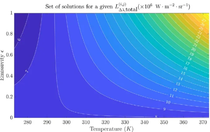
2.12 Possible solutions for a given measurement when everything but temperature and emis-sivity are known . . . 25
2.13 The geometry of the scene leads to different angle of view between the object and the camera in the image . . . 26
2.14 Different views of the same scene, the spatial sampling is not constant within the images 27 2.15 Mixed pixel effect illustration with three different materials. . . 28
2.16 Small uncooled IR camera with 3D-printed case. A coin of 1e is placed at the top as a scale factor. . . 29
2.17 Cross-sectional view of a bolometer pixel structure principle . . . 29
2.18 Different types of detectors reading . . . 31
2.19 Sensor / Object configuration . . . 31
3.1 Radiative transfer equation for satellite measurements, done at the top of the atmosphere. 37 3.2 ln approximation with its Taylor serie . . . 44 3.3 Original irradiance at sensor compared to the irradiance with the estimated emissivity
and temperature . . . 47 3.4 Found temperature and emissivity profiles . . . 48 3.5 Cubic spline interpolation with quadratic boundaries conditions. . . 49 3.6 Ray tracing images can be realistics, example with the POV-Ray software rendering . . . 61 3.7 Example of ray-traced rendering with the Sponza scene and Cycles open source renderer. 62 3.8 Monte-Carlo π approximation after 500 iterations and 10000 iterations. . . 63 3.9 Hierarchical subdivision . . . 65 4.1 Black-body calibration source . . . 73 4.2 Result of thermal calibration . . . 73 4.3 Principle of camera resectioning. . . 74 4.4 Extrinsics and intrinsics parameters over the camera resectioning. . . 75 4.5 Frame skew . . . 76 4.6 A comparison between the symmetric and reprojection error, as proposed in [85] . . . . 81 4.7 Result of interpolation after calibration and ROI recovering . . . 84 4.8 Spatial re-sampling influence . . . 85 4.9 HDF file recording format: different data type from various sensors can be registered
and then read back fastly due to the HDF internal architecture. . . 86 4.10 Any text file format can be imported and formated easily . . . 87 4.11 Parallelization of the temperature conversion process onto the GPU. Comparison of the
different implementations . . . 88 4.12 GUI of the tool . . . 89 4.13 YAML batch processing flowchart . . . 90 4.14 Road section instrumentation: IR image (a) and test site overview (b) . . . 90 4.15 Wood house instrumentation: IR image (a) and test site overview (b) . . . 91 4.16 Emissivity map for the wood house, colors represents one particular emissivity
measure-ment . . . 92 4.17 Effect of adjusting the emissivity for different material compared to a constant emissivity 92 4.18 Difference between true object temperature and estimated one depending on the error
made on the environment temperature and emissivity. In this case, the true object is at 293.15K and its emissivity is 0.93. How to read:on the left the true object’s temper-ature and emissivity. A point on the image represents the difference between the true object temperature and the estimated one with ˜Tenv(x-axis) and ˜ϵobj(y-axis) values. The images represent different environment temperatures values. . . 93
4.19 Comparison of ground truth temperature values to temperature estimation with and without sky correction . . . 94 4.20 Effect of using a correlation for the sky temperature based on the air temperature . . . . 95 4.21 Sky temperature derived from different sources of air temperature . . . 95 4.22 Difference between true object temperature and estimated one depending on the error
made on the atmospheric transmission. Here is the difference map for an object tem-perature of 293.15K and emissivity of 0.93. . . 96 4.23 Different distance values for the atmospheric transmission, through time. . . 96 4.24 Sun irradiance reflection on 7.5µm−13µm band for a normal object and different
emis-sivity values . . . 97 4.25 Sun irradiance reflection on 1.5µm − 5.4µm band for a normal object and different
emissivity values . . . 97 4.26 Comparison of sun’s irradiance measured and simulated on may 5th in the 0.3µm−
2.8µmband . . . 98 4.27 Rain and wind in-situ measurements . . . 98 4.28 IR image view: in dry environment (a), rain with optic issues (b) . . . 99 4.29 A set of environmental data for long-term thermal monitoring . . . 99 4.30 Comparison between the temperature estimation by considering Mtot = ϵobjMobj or
using the presented model and multi-sensor data . . . 100 5.1 Form factors for two infinitesimal elements . . . 102 5.2 Nusselt’s analog . . . 103 5.3 Gathering step as in the Gauss-Seidel algorithm, figure inspired from [40] . . . 108 5.4 Shooting step as in the Southwell algorithm, figure inspired from [40] . . . 110 5.5 Progressive radiosity examples with a Cornell’s Box where all surfaces emit in [1.5µm−
5.4µm]band. (a) Initial state. The ceiling source is at 353.15K and the objects at 293.15K with different emissivities. (b) After 10 iterations (≈ 0.15s). (c) After 100 iterations (≈ 0.3s). (d) After 1000 iterations with interpolation to smooth the result (≈ 4.4s). Almost all surfaces have shot their unshot radiosity (red texture). . . 111 5.6 OpenGL®pipeline. Blue boxes are programmable steps and dashed lines correspond to
optional stages [191]. . . 112 5.7 Mirror’s Edge Catalyst driven by Unreal Engine 3, which can interface OpenGL®-Credits to
deadendthrills.com . . . 113 5.8 Principle of the progressive radiosity GPGPU implementation . . . 114 5.9 Projection image of one of the plane from an element of the other plane . . . 117 5.10 Concurrency example. At first, the maximum value is 10 at index 0. The concurrency
makes the orders in the queues not the same. The maximum value is always guarantee but not its corresponding index . . . 119
5.11 Energy shot at a given time of the algorithm as a percentage of the first shot . . . 120 5.12 Signal received at the camera (left). Generated image by the camera (impulse response),
the digitization can be observed as well as the noises impact on the image. . . 120 5.13 Sun position over the sky vault for a 3D wood house scene . . . 122 5.14 Atmospheric model parameters in the software . . . 122 5.15 Spectrum of the solar irradiance received by a surface normal to the sun for different
visibility and altitude values . . . 123 5.16 Transmittance values for different zenith angles . . . 124 5.17 Effect of the pathlengths of ozone and N O2to their transmittance and comparison with
the original figure. . . 125 5.18 Animation of an object in the 3D scene through Python: an object on the scene is rotated
of 4 degrees and the scene is displayed on screen at each iteration. . . 126 5.19 Radiosity map of a building for a given day, at different time (from left to right: 6AM,
12PM and 4PM) . . . 127 5.20 3D model of the boogie in its scene environment . . . 127 5.21 Boogie and environment in the simulation software. The preview of the rendered
in-frared image is done in real-time at the bottom left corner. . . 128 5.22 Comparison of simulation data with experimental ones. The motion blur is well
repre-sented in the simulation. The temperature levels however are not well reprerepre-sented due to a lack of information about the initial temperatures values of the boogie. . . 128 5.23 Original and approximated reflectivity spectrum used for the validation . . . 129 5.24 Cornell’s box result for two different lights. Such result is computed on a professional
laptop - M1000M Nvidia graphic card, Intel i7-6820HQ CPU @ 2.70GHz. The computation time is approximately 60 seconds with a progressive rendering and aliasing on screen every 50 iterations. . . 129 5.25 Flowchart overview of the developed software showing the different steps of the
numer-ical simulation . . . 131 6.1 Temperature and emissivity profiles . . . 139 6.2 6-order Tchebychev approximation through Kalman filtering . . . 140 6.3 6-order Tchebychev polynomial approximation through combined Kalman filter and
gradient descent. . . 141 6.4 Kalman filter flowchart overview . . . 142 6.5 Temperature and emissivity estimation through the interacting Kalman filter (8000
par-ticles) . . . 146 6.6 Interacting Kalman filter flowchart overview . . . 147 6.7 Influence of the covariance kernel on the prediction (in black). The 95% confidence
6.8 Influence of the trend on the prediction (in black). The 95% confidence interval in light gray and the input measurements points in red. . . 154 6.9 Difference between a spherical and Matérn variogram models for a 2D problem . . . 155 6.10 Kriged Interacting Kalman filter flowchart overview . . . 159 6.11 Multi-resolution approach for solving the optimization problem. From left to right:
coarse level to highest final resolution details. . . 162 6.12 Comparison of the trust-region-reflective algorithm and the CMA-ES . . . 163 6.13 Cuboid’s result comparison . . . 163 6.14 Comparison of processing time, for one given scale with a given number of pixels . . . . 164 6.15 Target used for the study case. (a) Rendering of the scene in the visible spectrum. The
camera is represented, the target and the hemisphere for the environment. (b) Result example for a frame at 20◦Cand other materials at 5.2◦C . . . 165 6.16 Emissivity spectrum of the materials of the target. . . 166 6.17 Target material’s temperature evolution through time. The measurements correpond to
the temperature at ground during two days of january 2017. The decimated temperature profile is shifted by 1K for drawing purposes. . . 166 6.18 Focus on the emissivity retrieval on one pixel of each of the four materials for the 8µm−
12µm spectral band. . . 167 6.19 Results of the temperature / emissivity retrieval on one pixel of each of the four
materi-als. (a) (c) (e) (g): Emissivity retrieval. The ground truth profile (continous) is compared to the estimated one (per spectral band).(b) (d) (f) (h): Temperature estimation. The ground truth temperature is represented by the dashed line. . . 168 6.20 Initial prior for the CMA-ES optimization algorithm. A constant emissivity is chosen
leading to important differences with the ground truth values. Band: 10µm− 12µm. . . 169 6.21 Coarse level preliminary CMAES result. The image is blurry due to the level used. Band:
10µm− 12µm. . . 170 6.22 Full result of the CMAES algorithm at a given time and given band. At the opposite of
Fig. 6.21, the image is noisy due to the small neighborhood involved. Band: 10µm− 12µm.170 6.23 Filtered CMAES result after a 2D median filter. The materials have distinct emissivities
values on the emissivity map. As stated in Chapter 4 and observed on the temperature absolute difference image, a small error on low emissivity values can lead to important error in the temperature estimate. Band: 10µm− 12µm. . . 171 6.24 CMAES: SSIM and RMSE local values between estimated emissivity and temperature and
ground truth values. A small error on materials with low emissivity leads to a more important error in temperature than materials with higher emissivity. The material av-erage RMSE is up to 4K against 0.05 for the emissivity, which is still lower in avav-erage than for a constant emissivity case. Band: 10µm− 12µm. . . 172
6.25 Initial estimate by using a constant temperature value T = T0 = 270K. The emissivity at T0 is shown in the first image. The Kriged model result from this emissivity map is shown in the two other images with the mean estimate and standard deviation. Band: 10µm− 12µm. . . 173 6.26 Final estimate over the entire period. The ground truth values are compared to the
esti-mates. As for the CMA-ES the materials emissivities are distincts. Band: 10µm− 12µm. . . . 174 6.27 Estimated temperature time evolution at one pixel . . . 174 6.28 KIKF: SSIM and RMSE local values between estimated emissivity and temperature and
ground truth values. A small error on materials with low emissivity leads to a more important error in temperature than materials with higher emissivity. The material av-erage RMSE is less than 3K against 0.04 for the emissivity, which is still lower in avav-erage than for a constant emissivity case. Band: 10µm− 12µm. . . 175 D.1 A day forecasting with the SARIMA model used (2, 0, 0)× (0, 1, 1)1and its comparison
to actual measurements with the 95% confidence interval . . . 203 D.2 A day forecasting with the SARIMA model used (2, 0, 0)× (0, 1, 1)1and its comparison
1 Pseudo code for a Gibbs sampler . . . 54 2 Pseudo code for a slice sampling . . . 54 3 Pseudo-code of the SVD computation . . . 79 4 DLT based algorithm for calibration matrix estimation . . . 81 5 Pseudo-code for RANSAC algorithm where the error function and the model are defined
appart. . . 82 6 Pseudo-code for Jacobi radiosity solver . . . 107 7 Pseudo-code for Gauss-Seidel radiosity solver . . . 108 8 Pseudo-code for Southwell radiosity solver . . . 109 9 Pseudo-code for progressive radiosity . . . 111 10 Proposed code for progressive radiosities algorithm on hardware . . . 118
Introduction
I
nfrared thermography is a non-contact and full-field measurement technique used in numerous infrastructure diagnosis applications thanks to its non-invasive nature and large scale implemtation potential. In the context of energy savings, the thermal characterization of buildings en-velopes plays an essential role. Determining the thermal properties of a structure helps at refining and integrating various phenomena in diagnostics tools in order to measure its thermal efficiency but also its aging. Obtaining refined data on large infrastructures makes it possible to optimize repair costs, and thus save both energy and economic expenses. The latest improvements on uncooled infrared (IR) cameras have brought new opportunities for inexpensive thermal diagnostics in the Civil Engineering’s field. Although the technological maturity is ready, the methods to retrieve an accurate temperature measurement or at least with a known uncertainty are missing. In fact, the radiative flux that arrives at the camera’s sensors is not directly related to the observed target temperature. Instead, this flux depends on a combination of many parameters that varies with the 3D geometry of the scene, the me-teorological conditions, the self radiative properties of the objects, etc. In such context, the estimation of the temperature from those measurements is not trivial. If some parameters can be estimated from other local or online measurements, the most influential radiative quantity that will affect the temper-ature estimation is locally difficult to evaluate. This quantity is called the emissivity and depends on the object’s own characteristics (material, roughness), but also the angle of view and the temperature. As a consequence, in-situ infrared thermography for the thermal inspection of infrastructures is mainly used as a qualitative tool.The work done in this thesis aims at providing methods to estimate simultaneously the emissiv-ity and the temperature during long-term and in-situ multi-spectral infrared thermography measure-ments. One of the advantage of in-situ measurements is the presence of the sun as a natural heating source to excite the observed surfaces. Those various conditions coupled with long-term monitoring and multi-spectral measurements provide a set of data from which the emissivity and temperature can be extracted under some assumptions and statistical priors. Even more, a confidence interval is deducted to make the infrared thermography usable as a quantitative tool. In order to develop such method, the equations that govern the radiative heat transfer are introduced and presented in Chap-ter 2. The radiative phenomenon is complex and the equations are written at different observations scales to understand fully the assumptions used in the final model equation. In particular, it is shown that even if multi-spectral data brings more information to the system it is still insufficient to estimate
simultaneously the temperature and the emissivity.
A bibliographical review on the IR measurement process and radiative balance, the numerical sim-ulation of 3D thermal infrared scenes and the simultaneous estimation of emissivity and tempera-ture through multi-spectral infrared thermal measurements has been conducted. This bibliographical study, presented inChapter 3, highlights three ways to improve the temperature estimation accuracy. The first way is to correct the environmental effects and exploit in-situ complementary environ-mental measurements. InChapter 4, a description of how coupled environmental data measurements can improve the estimation result is presented. Moreover, when local measurements from multi-sensor acquisitions are not available, it is shown that open-data available online can also be exploited.
Then, in order to optimize new instrumentation solutions for in-situ studies and test developed emissivity and temperature estimation methods, a 3D simulation software tool has been developed and studied. This software, presented inChapter 5 is implemented on graphic hardware to reduce the computational time. It enables the numerical simulation of the radiative diffuses exchanges of 3D complex scenes. Thanks to an atmospheric spectral solar irradiance model and sun modelization, in-situ dynamic scenes can be simulated. Furthermore, the acquisition chain of the irradiance received at the camera sensor is also modeled and complete the measurement process simulation.
Developed mathematical models for the simultaneous estimation of the temperature and emissiv-ity are presented inChapter 6. Two methods from the literature have been implemented and three new methods are then proposed. The first one is an interacting Kalman filter which is the combina-tion of a particle filter on a Kalman filter. While the Kalman filter tracks the temperature evolucombina-tion through time, the particle filter estimates the model’s parameters. However, satisfying results are ob-tained only for small spectral bandwidth, which is suitable for hyper-spectral applications only. The second one is based on the covariance matrix adaptation evolution strategy (CMA-ES) meta-heuristic optimization algorithm. By assuming that on a given pixel’s neighborhood the temperature is homo-geneous, the equation system can be solved on a single-band image, at every moment. However, this robust method induces important computational costs. To overcome those previous issues, a combi-nation of an interacting Kalman filter with a spatial approximation is proposed. By using a priori on the spatial distribution of the emissivity through Kriging, a single-band or multi-band emissivity and temperature estimation method that tracks the parameters through time is proposed. Those methods are applied to a study case, obtained by the previous introduced simulation tool and compared.
Finally, conclusions and perspectives on in-situ infrared thermography for the monitoring of infras-tructures as well as obtained results are proposed and discussed.
Context and problem positioning
P
roposed methods in this thesis aim at making the temperature measurement of infrared ther-mal structure monitoring more accurate, or at least with a quantifiable error. This can only be achieved by identifying the surface properties of the observed object and in particular its emis-sivity, as exposed in this chapter. After introducing the concepts of the radiative transfer theory, the main equations to describe radiative exchanges in this thesis will be derived. Then, the main scientific challenges for in-situ infrared thermal monitoring are presented as well as the technological context on which this thesis is part of.2.1
Structural Health Monitoring (SHM)
Structural health monitoring aims at detecting and characterizing damages on engineering struc-tures. It has become a major public concern due to aging infrastructures and their intensive use [113]. A damage can be any change in the geometry or the material’s properties of the infrastructure system that may affect its performance. The system is observed over time thanks to various sensors. This gath-ered information is then exploited to prevent catastrophic events, save maintenance costs but also for prognostic. Therefore, SHM relies on multiple pillars (seeFig. 2.1). The first one concerns the diagnosis of the infrastructure through the observed physical phenomenon, which can be seen as an extension of Non Destructive Evaluation (NDE) [13]. The second one is the monitoring system in itself and all the parameters that defines it: sensors technology, acquisition architecture, data processing, communica-tion, etc. Therefore, SHM needs to consider the monitoring as a whole sub-system inside the structure: embedded and connected monitoring system integration, communication layers, power and even real-time data processing ability. All those elements need to reconsider the design and management of the structure to make it "smarter". Such complete systems have been studied for the monitoring of road transport infrastructures for example in [95], [176] or [49]. In those SHM applications, the monitoring is long-term, which needs to have a fully autonomous acquisition systems. Those systems are therefore critical for the monitoring and need to be scalable to any specific application. This implies to handle the various sensors [50], the amount of data to store, send [108] and process [63,62]. One concern about most civil engineering structures is their subject to environmental parameters due to their outdoor characteristic.
Figure 2.1: Main steps of structural health monitoring process
structures are subject to environmental parameters and more particularly to the solar flux, a natu-ral heating excitation source for the system [105]. Thermo-physical properties of the structure can therefore been followed through time. In this thesis, emphasis is given to the monitoring of infrastruc-tures through infrared cameras. In fact, infrared thermography cameras have experienced significant technological development over the last decade. Uncooled cameras with good resolution, relatively inexpensive and even multi-spectral are now possible [193]. Infrared thermography offers an interest-ing solution to monitor structure’s thermal evolution through time. First, infrared cameras provide a non-contact and non-destructive technique which simplifies the setting up on field. Then, infrared thermography offers a multi-point measurement with a large field of view, suitable for large scale structures [36]. However, in-situ infrared measurements are often used as qualitative data only [80]. In fact, the measured flux that arrives at the sensor depends on the surrounding and meteorological environment (seeSection 2.4.1andChapter 4). As a consequence, complementary data measurements are needed to estimate the temperature of the observed object. The objective of this thesis is to use this multiple sensors configuration and propose a method to estimate the temperature with a known uncertainty. The sensitivity of the measurement model to its different parameters will be studied on actual measurements.
Some elements of the thermal radiative transfers theory are given in the following section. This theoretical background will be used to derive the equations that govern the main phenomena that
occur during infrared thermography.
2.2
Thermal radiative transfers
Radiation transfer is one of the three means for thermal energy to be transferred with conduction and convection. The diffusion represents the transfer of heat via molecular interactions whereas radi-ation represents the transfer of heat via photons/electromagnetic waves. The radiative transfer theory (RT) aims at studying the absorption, emission and scattering of electromagnetic radiation as it passes through a medium. Such interactions can be described mathematically by the equation of radiative transfer. RT is involved in a wide variety of fields, including remote sensing, atmospheric science, as-trophysics, optics etc. The purpose of this section is to provide the main principles of the RT theory and to introduce its concepts through the equations. Those definitions and a more detailed description of RT theory can be found in standard textbooks [93,26,53]
2.2.1 Radiative transfer theory
For the purposes of this study, radiation is viewed as the transport of energy in electromagnetic waves. All substances continuously emit electromagnetic radiation due to the different interactions and motions of the molecules and atoms they are made. The term thermal radiation is reserved for the visible and infrared portion of the spectrum since the related radiation should be detected by either heat or light [23]. The infrared part of the electromagnetic spectrum is given inFig. 2.2.
Figure 2.2: Focus on the IR part of the electromagnetic spectrum. Common spectral bands of IR are shown: Near-infrared (NIR: 0.75− 1.4µm); Short-wavelength infrared (SWIR 1.4 − 3µm); Mid-wavelength infrared (MWIR 3−8µm); Long-wavelength infrared (LWIR 8−15µm); Far infrared (FIR 15−1000µm). The atmospheric transmission is also represented.
transmitted (also, those effects can affect the frequency of the radiation beam). All those different in-teractions make the thermal radiation a complex phenomenon. Absorption and scattering effects can be studied on their own: the size of the particle relative to the wavelength of the radiation, the index of refraction (complex) of the material and also the shape of the particle will have an impact on the scattered proportion of the incident radiation. All of this leads to the study of different parameters such as the particle’s phase function, the scatter cross section and the absorption cross section. The pur-pose of this study is not to go too deeply in the description of all the physical effects that occur since it will make the approach too complicated. However, it is still important to know that other physical phenomena exist at lower scales that cannot be taken into account in the presented models. For more readings on this subject, see [182] and [21]. Two approaches can be used for describing the radiation theory: the classical electromagnetic theory and quantum mechanics. Whereas quantum mechanics will take into account the microscopic interactions of the radiation with matter, the classical theory such as Maxwell’s equations will only derive the macroscopic behavior. As explained before, we cannot go too deeply onto lower scales since the mathematical complexity of the approach will increase and become unusable for practical study cases. Therefore, a combination of the two approaches is generally used in the litterature. For example, the spectral intensity is derived from the photon model whereas the absorption, transmission and emissivities are considered from a more classical approach as con-stant of proportionnality in the equations. This is why most of the time those parameters are derived from experimental studies even though they could be developed by the quantum mechanics through Einstein’s transition probability coefficients. In such context, the main physical quantities involved into the RT theory and mainly described in [93] will be presented. Then, based on those definitions, the different radiative transfer equations will be derived.
2.2.2 Basic radiation properties
Let first start by giving some definitions on temperature. One can define temperature differently [16]:
• Thermodynamic temperature: T is defined according to the second principle of thermodynamics, for a medium in thermal equilibrium, which can be measured directly by a thermometer. For non-isothermal bodies, the temperature T (x, y, z) is defined as the temperature of an elementary isothermal volume at the location (x, y, z). The surface temperature is then defined by the limit of T (x, y, 0) with a width approaching zero.
• Radiometric temperature: This time, the temperature is defined from the radiance Lλemitted by a surface and defined later on in this chapter. The radiance Lλmeasured by a radiometer may be written with appropriate approximations and the temperature retrieved from those equations. It is important to note that the surface temperature is well-defined for homogeneous materials at ther-mal equilibrium. However, it becomes much more complicated when considering non isotherther-mal and heterogeneous materials. Most of the time in this thesis, the materials will be considered homogeneous
and that thermal equilibrium is reached.
Radiation can be viewed as the transport of energy by discrete photons for which the relationship between its energy and frequency ν (or wavelength λ = c/ν) is given by Planck’s relation:
ϵ = hν = hc
λ (2.1)
where h is Planck’s constant and c the speed of light in vacuum. Eq. (2.1)shows an interesting fact: the energy of the radiation is inversely proportional to the radiation wavelength. This property can be easily observed by looking at the change of a burning flame as it goes hotter. Hotter temperatures mean higher energy which leads to a shift in frequency and therefore, in its color. In the XIXthcentury, the Stefan-Boltzmann law was established, deriving the maximum emission value for a given surface at a given temperature.
Definition 2.2.1 (Stefan-Boltzmann Law). We can describe the power radiated from the black-body in terms of its temperature:
M◦(T ) = σT4 (2.2)
This relation describes the power radiated from a black body surface (denoted with the superscript ◦) which depends only on the temperature of the surface and is expressed in W/m2. All real surfaces will emit radiation at a rate smaller than M◦which represents an ideal surface called black body (more details on black body and real surfaces radiation will be given in the next section). Then, at the be-ginning of the XXthcentury, Planck showed that the radiative energy emitted by a black body could be expressed over the spectrum a relation now called the Planck’s law.
Definition 2.2.2 (Planck’s law). Planck’s law describes the radiative energy emitted by a black body to its temperature (T ) over the spectrum through the Planck’s function denoted L◦λ(T ). An increase of temperature will lead to an increase of the emitted frequency.
L◦λ(T ) = 2hc 2 λ5 1 e hc λkB T − 1 (2.3)
Two constants are often used to simplify the writing of Planck’s law C1 = 2hc2and C2 = khcB:
L◦λ(T ) = C1 eC2λT − 1
(2.4)
By integrating Planck’s Law over the spectrum, the Stefan-Boltzmann law is found:
∫ ∞
0
L◦λ(T )dλ = σT4 (2.5)
Fig. 2.3shows the Planck’s law as a function of wavelength, for different temperatures values. The maximum of this distribution is shifted as the temperature changes. This is known as the displacement
Figure 2.3: Planck’s law as a function of wavelength at different temperature values
law of Wien: the wavelength that maximizes the emission relies on the temperature but the product λmax(T )T ≈ 2.898 × 10⁻³mK remains constant. Such property explains why an incandescent bulb filament emits in the red at about 700◦Cand becomes white and then blue for higher temperatures.
At the same time, two other relations linking the radiative energy emitted by a black body were found the Rayleigh-Jeans formula and the Wien’s approximation law. Both of those formulae can be retrieved by Planck’s law and may be used for particular applications as an approximation of Planck’s law.
Definition 2.2.3 (Rayleigh-Jeans formula). By expanding the exponential of the denominator ofEq. (2.21) in a series: eλkThc = ∞ ∑ n=0 (λkThc )n n! , ∀ hc
λkT > 0(always the case) (2.6)
For λT >> hc
k, we can approximate the denominator by using the development until n = 1 which gives:
L◦λ(T ) = 2ckT
λ4 (2.7)
Definition 2.2.4 (Wien’s approximation law). This was the model originaly proposed by Wien to de-scribe the complete spectrum of thermal radiation until Planck’s one.
Wien’s approximation can now be derived from Planck’s law when hν ≫ kT : L◦λ(T ) = 2hc 2 λ5 1 e hc λkB T − 1 ≈ 2hc2 λ5 e −hc λkB T (2.8)
The temperature of a black body can therefore be deducted from Planck’s law:
T = C2 ln ( (C1+λ5M◦ λ)λ (λ5M◦ λ)λ ) (2.9)
Figure 2.4: Temperature as a function of exitance at different wavelengths.
Fig. 2.4shows the temperature value as a function of radiant exitance, for different wavelength values. This figure shows two main trends regarding the temperature and exitance dependence. In the MWIR-LWIR bands, highest energy levels correspond to a more important increase of the temperature than in the NIR-SWIR bands.
In the next section, the main quantities of the radiative transfer theory will be defined in order to derive - at the end - the radiative transfer equations and get a better understanding of this physical phenomenon.
Wien’s approximation is often used to approximate Planck’s law and partic-ularly to linearize the equation system as shown on the emissivity - tem-perature section. This approximation can be justified in common civil en-gineering applications: since hc
k = 14388µm· K, in the LWIR band (λ ∈ [8µm; 14µm]), we must have 959.2 >> T .
Note
2.2.3 Radiative transfer quantities definitions
Radiative transfer represents exchanges between surfaces and inside medium. Due to the complex-ity of the phenomenon it is important to keep in mind that the radiative transfer deals with waves that propagate among surfaces and through a medium. Therefore, the surfaces particularities and the ge-ometry between the surfaces will have an effect on this heat transfer. To describe those exchanges, it is necessary to remind the solid angle definition.
Definition 2.2.5 (Solid angle). The solid angle is an equivalent of the planar angle but in three-dimensional space. It represents a part of 3D space delimited by a cone (the vertex of the cone is the vertex of the solid angle). It is a measure of the field of view from a particle point that an object covers and therefore used in radiometry to determine the exchanges between two bodies. The solid angle is defined as the ratio of its base area to the square of chord length. Its dimension is the steradian sr:
dΩ = A
r2 (2.10)
The solid angle can also be defined on an unit hemisphere, which will be used later on (seeFig. 2.5):
dΩ = rdθr sin(θ)dΦ
r2 = sin θdθdΦ (2.11)
In radiometry, the quantities are defined for a given solid angle, to represent the beam direction. However, for approximation and simplicity needs or sometimes due to uniformity, the quantities may be referred to as hemispherical. In that case, it means that the quantity is integrated on the unit hemi-sphere over the surface. Hemispherical properties get rid of the angle component and propose a more global representation of the quantity, as an average over the surface.
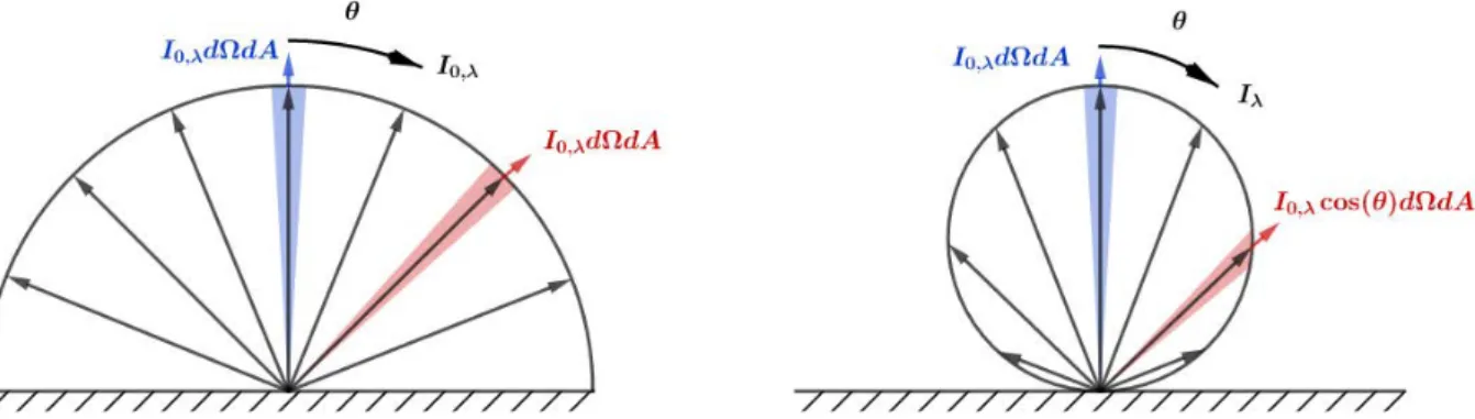
Definition 2.2.6 (Radiance). The analysis of radiation field deals with the analysis of the amount of energy dQλ(x, Ω, t)that is transported across an element of area dA [26]. The radiation will then be highly dependent on the spatial geometry and the location of this area element. Let D ⊂ Rd(d ∈ {2, 3}) and A be the unit sphere of Rd. This energy is defined by unit of projected surface, dA cos(θ)
Figure 2.5: Solid angle on hemisphere. Note that the solid angle is not necessary a circular cone
to be located at x in time dt, in the solid angle dΩ about the direction ⃗n in the wavelength interval [λ; λ + dλ]:
dQλ(x, Ω, t) = Lλ(x, Ω, t) cos θdλdAdΩdt (2.12)
where θ is the angle which the direction considered makes the outward normal to d⃗n. The quantity Lλ(x, Ω, t)is called spectral radiance (W· sr−1· m−2· µm−1) We have to note the fact that Lλ(x, Ω, t) depends on seven variables in total:
• 3 variables giving the position in space x,
• 2 variables giving the direction of the radiation Ω, in which we use the inclination angle θ and the azimuth angle φ,
• The time variable t,
• The wavelength λ or sometimes the energy hν or the frequency ν = c λ.
This dimensionality makes the solving of the general radiative transfer equation difficult both analyti-cally and numerianalyti-cally. Moreover, most of the time, the radiation has an impact on the crossed material, which also has an impact on the incomming radiation. Therefore, the resolution of the problem must be coupled, iteratively.
depends on, we may abusively write1:
Lλ ≡ Lλ(x, Ω, t) (2.13)
Definition 2.2.7 (Radiant flux). Radiant flux is the radiant energy emitted, reflected, transmitted or received, per unit of time (W).
ϕ = ∂Q
∂t (2.14)
where Q is the radiant energy emitted, reflected, transmitted or received (J). FromEq. (2.1)we can define the spectral flux in frequency ϕν = ∂ϕ∂ν and the spectral flux in wavelength ϕλ= ∂ϕ∂λ1.
Finally, one can combineEq. (2.4)andEq. (2.1)to get the spectral radiance in terms of flux which represents how much of the power is emitted, reflected, transmitted or received by a surface when an optical system is looking at the surface from a specified angle of view as unit.
Lλ =
∂2ϕλ
cos(θ)∂Ω∂A (2.15)
where:
• ϕλis the radiant spectral flux (emitted, reflected, transmitted or received), • Ω is the solid angle,
• ∂A cos(θ) is the projected surface.
Definition 2.2.8 (Irradiance). The irradiance denoted E is defined as the local value of the ratio of the flux ϕr received by an object and the area of this object. It is the power received per unit area (W· m−2):
E = ∂ϕr
∂A (2.16)
Definition 2.2.9 (Exitance). The radiant exitance denoted M is defined as the local value of the ratio of the flux ϕe emitted by an object and the area of this object. It is the power emitted per unit area (W· m−2):
M = ∂ϕe
∂A (2.17)
Definition 2.2.10 (Radiosity). The radiosity of a surface denoted J is the radiant flux leaving (emitted, reflected and transmitted by) a surface per unit area. It is the power left per unit area (W· m−2). Therefore:
J = ∂ϕ
∂A = M + Jreflected+ Jtransmitted (2.18) When the surface is opaque, Jtransmitted = 0 =⇒ J = M + Jreflected.
Definition 2.2.11 (Radiant intensity). The radiant intensity is the ratio of the flux ϕeemitted per unit solid angle dΩ:
I = ∂ϕe
∂Ω (2.19)
As explained in [93], the intensity of radiation from a black-body is defined on the basis of the nor-mal area. It means that I is independent of the direction of emission, by definition which enables the description of a black-body intensity without defining the normal of the surface or the angles (θ, Φ).
Definition 2.2.12 (Directional emissive power). The radiant intensity is defined by its normal which means that the maximum energy emitted by a surface is reached if the surface is normal to the receiver. When there is an angle between the two surfaces, then the energy reaching the receiver is not the radiant intensity anymore. By assuming that the emission is uniform in all directions, the directional spectral emissive power for a black surface can be derived:
˜
I(θ, Φ) = I cos(θ) = ˜I(θ) (2.20)
where ˜Istands for the directional emissive power. This equations is valid for Lambertian surfaces which represent a perfect diffusion: the brightness of the surface appears the same no matter the observer’s angle of view (Fig. 2.6). The emission is therefore isotropic and the intensity followsEq. (2.20)called Lambert’s cosine law.
Figure 2.6: Emission rate in a normal direction and off direction with the Lambert’s cosine law on the right.
Based on this law, one can integrate the emission of a black-body through a unit hemisphere over the surface. The spectral emission from an infinitesimal area dA per unit of time and unit surface area passing through the element on the hemisphere is given by:
˜
By integrating over the hemisphere and usingEq. (2.20) ˜ Iλdλ = Iλdλ ∫ 2π Φ=0 ∫ π 2 θ=0
cos θ sin θdθdΦ = πIλdλ (2.22)
The black-body hemispherical emissive power is therefore π times the black-body intensity. We also have the equivalent in luminance. For a flux leaving the surface in an isotropic way:
Mλ= πLλ (2.23)
Definition 2.2.13 (Bouguer’s law). Finally, Bouguer’s law defines the relation between the irradiance E of a receiving surface, due to a source S and the intensity of that source in the direction of the receiver lying at a distance d. In the case of a nonparticipating media.
E = I cos(θ)
d2 (2.24)
The Lambert’s cosine law can be recognized in this expression as well as the inverse square law. Now that the main quantities that describe the radiation theory have been introduced, the next section aims at developing the principles behind the actual phenomena that occur at a given surface.
2.2.4 Surface properties
Until now, the black body has been said to be a body that emits the maximum of energy for a given temperature. To be more accurate, a black body is an idealized physical body that absorbs all incident electromagnetic radiation, regardless of the frequency or the angle of incidence [144]. At the oppo-site of a black body, a white body will reflect all incident rays uniformly and entirely in all directions. Whereas black body represents an idealized object, real materials are considered to emit energy at a fraction of a black body energy levels. The ratio that links the two materials is called emissivity (ϵ, more rigorously defined later on). Finally, surfaces that have their properties independent of wavelength are called grey surfaces. When dealing with real radiating materials, multiple interactions at interfaces may occur and are schematized inFig. 2.7. The emission has been defined previously for a black body, as well as the incident radiation. However, the reflectivity, absorption and transmission have not been mentioned yet and are addressed in this section.
To understand well the complexity of those phenomena, it is necessary to view those quantities as local properties of the material. As for the previous quantities, they will depend on the solid angle, the wavelength and the temperature but also on the intrinsic characteristics of the surface’s material. Wood and metal will not absorb or reflect the same way; as well as polished iron will not have the same properties as unpolished one. From a practical point of view, giving values to those quantities is difficult. In fact, when the reflection or the absorption of a given material is given in the literature


![Figure 2.9: Effect of the state of the surface on emissivity (from [71]) the radiation [93]:](https://thumb-eu.123doks.com/thumbv2/123doknet/14596377.730538/45.892.85.769.169.449/figure-effect-state-surface-emissivity-radiation.webp)