HAL Id: hal-00173580
https://hal.archives-ouvertes.fr/hal-00173580
Submitted on 12 Feb 2010
HAL is a multi-disciplinary open access
archive for the deposit and dissemination of
sci-entific research documents, whether they are
pub-lished or not. The documents may come from
teaching and research institutions in France or
abroad, or from public or private research centers.
L’archive ouverte pluridisciplinaire HAL, est
destinée au dépôt et à la diffusion de documents
scientifiques de niveau recherche, publiés ou non,
émanant des établissements d’enseignement et de
recherche français ou étrangers, des laboratoires
publics ou privés.
Lookahead Computation in G-DEVS/HLA Environment
Gregory Zacharewicz, Claudia Frydman, Norbert Giambiasi
To cite this version:
Gregory Zacharewicz, Claudia Frydman, Norbert Giambiasi.
Lookahead Computation in
G-DEVS/HLA Environment. SNE Simulation News Europe, ArgeSIM, 2006, 16 (2), pp.15-24.
�hal-00173580�
1
S
IMULATION
N
EWS
E
UROPE
Speci
al Issue 1
Lookahead Computation in G-DEVS/HLA Environment
Gregory Zacharewicz Claudia Frydman Norbert GiambiasiLSIS UMR CNRS 6168 Université Paul Cézanne Marseille France
{
{ggrreeggoorryy..zzaacchhaarreewwiicczz;;nnoorrbbeerrtt..ggiiaammbbiiaassii;;ccllaauuddiiaa..ffrryyddmmaann}}@@llssiiss..oorrg g
Abstract
In this article, we present new methods to evaluate lookahead of DEVS/G-DEVS federates participating in a HLA federation.
We propose first, an algorithm to compute the loo-kahead according to the current state of a DEVS/G-DEVS model. This solution is designed for models with lifetime function depending on one state variable.
Then, we extend this computation to models with lifetime functions defined with several state variables. We use the Dijkstra graph theory search to compute the different values of state variables and a mathe-matical function analysis to determine the lookahead for the model states. Finally, we illustrate with an ex-ample how this solution extends the range of DEVS/G-DEVS models that can be involved into dis-tributed simulations and we present some simulation results.
1. Introduction
On the one hand, G-DEVS [7] lies in its ability to develop uniform discrete event executable specifica-tions for hybrid dynamic systems with a scientifically controlled degree of accuracy. Hence, models of con-tinuous and discrete components can be represented with the same formalism using only a continuous time representation.
On the other hand, HLA [16] allows integrating dis-tributed simulations, located on several computers with different operating systems, into a global simula-tion. HLA-compliant distributed simulations intercom-municate by exchanging messages eventually syn-chronized.
A first DEVS/HLA compliant environment was pro-posed by Zeigler et al. in [20,21]. In this environment, distributed DEVS simulations intercommunicate through the interface (RTI) specified by HLA. In [14], Lake et al. have proposed a DEVS/HLA environment improvement by using the HLA lookahead. In [18], we have proposed a DEVS/HLA environment using the HLA lookahead without moving the management of the coupling relations from the RTI level to the feder-ate level as in [14].
The focus of this article is to improve the DEVS/HLA environment proposed in [18]. For that purpose, in a first part, we compute a lookahead
de-pending on the current state of DEVS models with life-time function depending on only one state variable. It allows increasing the value of the HLA lookahead.
Then, we propose going further in the improve-ment of the HLA lookahead computation. This compu-tation tackles DEVS/G-DEVS models for which state lifetimes are functions of more than one state variable. This lookahead computation is based on the shortest and longest path search algorithms in a graph. This improvement permits to compute non-zero HLA loo-kahead values from models with complex lifetime functions. This result is significant because the use of greatest values for the lookahead improves the per-formances of distributed simulation according to litera-ture on distributed discrete event simulation [5].
This article is organized as follows. Section 2 gives a brief recall on DEVS/G-DEVS formalisms and HLA standard. Section 3 recalls previous DEVS/HLA map-ping. Section 4 exposes the approach proposed for improving the lookahead computation of the DEVS/G-DEVS HLA environment. Finally, we conclude by giv-ing some simulation results that illustrate the perform-ances of the proposed algorithm.
2. Recall
2.1 Generalized Discrete EVent System Specification (G-DEVS)
Traditional discrete event abstraction (e.g. DEVS) approximates observed input-output signals as piece-wise constant trajectories. G-DEVS defines abstrac-tions of signals with piecewise polynomial trajectories [7]. Thus, G-DEVS defines coefficient-event as a list of values representing the polynomial coefficients that approximate the input-output trajectory. Therefore, a DEVS model is a zero order G-DEVS model (the in-put-output trajectories are piecewise constants). For-mally, G-DEVS represents a dynamic system (DESN)
as an n order discrete event model expressed as a structure:
DESN = <XM, YM, S, δ int, δ ext, λ, D, Coef>
The following mappings are required:
XM = A n+1, where A is a subset of integers or real numbers that represents external input events
YM = A n+1, represents output events
S
IMULATION
N
EWS
E
UROPE
Speci
al Issue 1
Speci
al Issue 1
Where Q is a set of state variables, and A n+1 is a
subset of state variables that stores last input coeffi-cient-event.
For all total state (q, (an, an-1,..., a0), e) (with e:
elapsed time in S, 0 ≤ e ≤ D(S)) and a continuous polynomial input segment w : <t1, t2> → x, the
follow-ing functions are defined :
The internal transition function: that defines the
autonomous state changes for the transient states, (i.e. states for which lifetime is a finite value):
δint(S) = δint (q, (an, an-1,..., a0)) =
Strajq, x (t1+D((q, (an, an-1,..., a0)), x))
with x =antn+an-1tn-1+…….+a1t+a0
and Straj is the model state trajectory ∀ q ∈ Q and ∀ w : <t1, t2> → x,
Strajq,w : <t1, t2> →Q
The external transition function: that defines the
state changes caused by external events: δext(S, e, XM) =
δext (q, (an, an-1,.., a0), e, (an’, an-1’,.., a0’)) =
Strajq, x ((t1+e), x’)
with: Coef (x) = (an, an-1,..., a0)
and Coef (x’) = (an’, an-1’,..., a0’)
Coef: function to associates n-coefficient of all
con-tinuous polynomial function segments w over a time interval <ti, tj>, to the (n+1) constants values (an, a n-1,..., a0) such as:
w(t) = antn+an-1tn-1+….+a1t+a0
Coef-1: the inverse function of Coef is applied to transform an output event in piecewise continuous polynomial trajectory:
Coef-1 (an, an-1,..., a0) = antn+an-1tn-1+….+a1t+a0
The output function: triggered by autonomous state
changes, it produces output events:
λ(S) = λ (q, (an, an-1,..., a0)) = (an’, an-1’,.., a0’)
The function defining the lifetime of states: that
represents the maximum length or lifetime of a state:
D(S) = D (q, (an, an-1,..., a0)) =
MIN (e/Coef (Otrajq, x (t1)) ≠
Coef (Otrajq, x (t1 + e))
with Otraj is the model output trajectory: Otrajq,w : <t1, t2> →Y
2.2 DEVS / G-DEVS Coupled Model
Zeigler has introduced, in [23], the concept of cou-pled model. Every basic model of a coucou-pled model interacts with the other models to produce a global behaviour. The basic models are, either atomic mod-els, or coupled models stored in a library. The model coupling is done using a hierarchical approach. A dis-crete event coupled model (DEVS or G-DEVS) is de-fined by the following structure:
MC = < X, Y, D, {Md/d∈D}, EIC, EOC, IC, Select>
X: set of external events. Y: set of output events. D: set of components names. Md: DEVS/G-DEVS models. EIC: External Input Coupling relations. EOC: External Output Coupling relations. IC: Internal Coupling relations.
Select: defines priorities between simultaneous events intended for different components. Note that to allow the coupling of different degree models ports, Giambiasi et al. have defined, in [7], a coupling model component to transform the polyno-mial order of events exchanged.
2.3 DEVS / G-DEVS Simulator
The concept of abstract simulator has been pro-posed in [23] to define the simulation semantics of the formalism. The architecture of the simulator is derived from the hierarchical model structure.
The processors involved in a hierarchical simula-tion are Simulators, which insures the simulasimula-tion of the atomic models, Coordinators, which insures the routing of messages between coupled models, and the Root Coordinator, which insures the global man-agement of the simulation (e.g. Fig. 1. a, without con-sidering crosses out).
The simulation runs by exchanging specific mes-sages (corresponding to different kind of events) be-tween the different processors.
2.4 The High Level Architecture (HLA)
The High Level Architecture (HLA) is a software architecture specification for global simulations that can include a variety of simulation programs imple-mented on distant computers and/or to reuse existing simulations by interconnecting them [6]. Dr. Straßburger presents in this journal an overview of this specification [16].
2.4.1. Implementation Components. An HLA
federa-tion simulafedera-tion is composed of federates and a Run time Infrastructure (RTI) [11].
A federate is a HLA-compliant program, the code of that federate keeps its original features but must be
3
S
IMULATION
N
EWS
E
UROPE
Speci
al Issue 1
extended by other functions to communicate with other members of the federation. These functions, contained in the HLA-specified class code of
Feder-ateAmbassador, make interpretable by a local
proc-ess the information received resulting from the federa-tion. Therefore, the federate program code must in-herit of FederateAmbassador to complete abstract methods defined in this class used to receive informa-tion from the RTI.
The RTI supplies services required by a simula-tion, it routes messages exchanged between feder-ates. It is composed of two parts.
The “Local RTI Components code” (LRC, e.g. in Fig. 1 b) supplies external features to the federate for using RTI call back services such as the handle of ob-jects and the time management. The implementation is the class RTIAmbassador, this class is used to transform the data coming from the federate in an in-telligible format for the federation. The federate pro-gram calls the functions of RTIAmbassador to send data to the federation or to ask information to the RTI. Each LRC contains two queues, a FIFO queue and a time stamp queue to store data before delivering to the federate.
Finally, the “Central RTI Component” (CRC, e.g. in Fig. 1 b) manages the federation notably by using the information supplied by the FOM [16] to define Ob-jects and Interactions classes participating in the fed-eration. Object class contains object-oriented data shared in the federation that persists during the run time, Interaction class data are just sent and received.
A federate can, through the services proposed by the RTI, "Publish" and "Subscribe" to a class of shared data. "Publish" allows to diffuse the creation of object instances and the update of the attributes of these instances. "Subscribe" is the intention of a fed-erate to reflect attributes of certain classes published by other federates.
2.4.2. HLA time management. In order to respect the
temporal causality relations in the simulation stated in [15]; HLA [4,5] proposes classical conservative [1,2] or optimistic [12] synchronization mechanisms. We focus in this article on conservative synchronisation and event driven mechanism.
We recall here the time management notions from [9,10,11], implemented in the 1516 compliant RTI im-plementation, that will be exploited in the following of this article:
Lookahead: Delay given by influencers federates
to the RTI. They certify to the RTI not to emit message until their actual time plus their lookahead.
GALT (Greatest Available Logical Time): Time
stamp, computed by the RTI, until influenced feder-ates will not receive information from the federation (i.e. minimum lookahead of its influencers federates).
NextMessageRequest(t) (NMR(t)): Federate
func-tion to ask for grant to the RTI, to deal an event time stamped t. If the RTI call-backs the federate with
TimeAdvanceGrant(t), this federate is sure to have
received all events at t’ ≤ t and can emit events time stamped t’’ > t.
NextMessageRequestAvailable(t) (NMRA(t)):
dif-fers from NMR(t) in the call-back function.
TimeAd-vanceGrant(t) answer to NMRA(t), ensures the
feder-ate to have received all events at t’ < t and allows it to emit events at t’’ ≥ t. In return, the federate is not sure to have received all events time stamped t.
LITS (Least Incoming Time Stamp): Federate LITS
is a lower bound until which the federate will receive no message, this value is calculated from its GALT and the messages in transit not received yet by the federate (i.e. messages stored in the LRC queue).
3. Previous DEVS/HLA mapping
3.1 Components mapping
Zeigler et al., in [20,21,22], present a first integra-tion of DEVS Coordinators in a HLA-compliant archi-tecture. They map local coupled models in HLA feder-ates whose coordinators of higher level will have re-sponsibility to communicate with a “Time Manager” federate. TM routes messages between distributed coordinators. This federation of coordinators defines a global distributed coupled model.
3.2 Integrating Algorithms
As recalled in the previous section, deterministic distributed simulations require synchronization mechanisms in order to treat events in respect to cau-sality. In consequence, DEVS/HLA federates must include integrating algorithms to communicate with the RTI (i.e. in order to handle received messages from the federation and to emit messages in a HLA format).
Zeigler et al. have proposed in [22] a first integrat-ing algorithm of DEVS models into a HLA-compliant environment. To guarantee the global synchronization of Local Coordinators, this approach exploits conser-vative algorithm of [1,2] mechanism available in HLA [11].
In [14], Lake et al. have given a second approach for mapping DEVS into HLA that resolves Deadlock problems encountered in the first solution. To this end, this approach notably uses the NMRA(t) service pro-posed by HLA instead of NMR(t). This two solutions use a zero or negligible value of HLA lookahead for every federate [4].
S
IMULATION
N
EWS
E
UROPE
Reference [14] also introduced another approach that uses a not negligible lookahead by globally broadcasting event messages among federates and giving to each federate a global view of DEVS cou-pling relations. So, the federates decide to treat or not an event regarding to their history of received events and to their knowledge of coupling relations. This DEVS/HLA environment uses a non-zero constant for the lookahead. However, some responsibilities of the RTI are transferred to the federates, what bypasses some RTI functions.
4. New G-DEVS/HLA mapping
4.1 Components mapping
We have proposed, in [18], an environment for creating DEVS/G-DEVS models HLA compliant. This environment proposes two-step for distributing models (and simulators associated to).
In the first step, the GDEVS coupled model is flat-tened. The hierarchical structure of a model is a user facility, which is not necessary adapted to a simulation purpose. This new simulation structure decreases the algorithm complexity and so increases simulation per-formance regarding to the hierarchical one as stated by Kim et al. and Glinsky et al. in [8,13]. The flattening of the structure induces eliminating the crossed out Coordinators on Fig.1 a.
In the second step, the flattened G-DEVS simula-tion structure is split into coupled model by federate (Fig.1 b) in order to build an HLA federation (i.e. a dis-tributed G-DEVS coupled model). The environment conforms to [22] mapping of Local Coordinator and Simulators into HLA federates, but does not use the
“Time Manager” federate. It maps directly the Root Coordinator into the RTI. The reason of this mapping is the specification of interface (RTI) proposes ser-vices that enclose those defined in the DEVS Root Coordinator. Thus, the “global distributed” model (i.e. the federation) is constituted of federates intercom-municating.
The G-DEVS models federates intercommunicate by publishing/subscribing to HLA interactions that map the coupling relations of the global distributed coupled model. This information is routed between federates by the RTI in respect to time management and FOM description.
4.2 G-DEVS/HLA integrating Algorithms
From the first algorithm of [14], we have proposed in [18] a solution integrating the use of the HLA looka-head. This solution can be applied to G-DEVS or DEVS coupled model. It considers a local G-DEVS coupled model integrated in a HLA federate. This fed-erate communicates with other G-DEVS models within the federation. We set the federate lookahead as in function (1).
Lookahead = Min D(s) / s ∈ S (1) Where S is the set of model states.
We assume to use, G-DEVS models with D(S) > 0 to define a non-zero lookahead.
Moreover, we state that, in the case of simultane-ous events, we choose to treat first the internal event, then, after having emitted an output event and done a state change, we process simultaneous external events using a confluent function.
Root Coordinator Coordinator B Coordinator D Coordinator C Coordinator A Simulator B1 Simulator D1 Simulator C1 Simulator D2 Root Coordinator Coordinator B Coordinator D Coordinator C Coordinator A Simulator B1 Simulator D1 Simulator C1 Simulator D2 a) Interconnection Network b) Central RTI Component Simulator B1 Simulator C1 Simulator D2 Simulator D1 Computer 1 Computer 2 Computer 3 Local Coordinator AB Local Coordinator ACD Local RTI Component Local RTI Component Federate 1 Federate 2 Speci al Issue 1 Speci
5
S
IMULATION
N
EWS
E
UROPE
Speci
al Issue 1
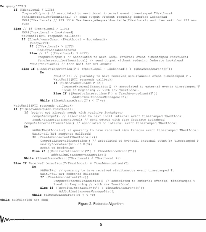
We recall from [18], in the Fig. 2 pseudo-code, the federate algorithm to communicate with the RTI. The initial settings define that the actual logical time of this federate is “Tact” and it possesses a next local event planned in its local event list at “TnextLocal”. It uses the queryLITS() RTI service defined in the HLA stan-dard. Using this service, a federate can preserve a non-zero lookahead value by treating local events with timestamps earlier than LITS (that evolves depending
on influencers federates data delivering behaviour and processing speed). In consequence, a non-zero loo-kahead federate frees of constraint federates under its influence for a period equal to the lookahead. Thus, this situation increases the parallelism of the global simulation.
It should be noted that our pseudo-code is de-signed for the 1516 version of HLA specification and the 1516 compliant RTI implementation.
Do queryLITS()
If (TNextLocal ≤ LITS)
ComputeOutput() // associated to next local internal event timestamped TNextLocal SendInteraction(TnextLocal) // send output without reducing federate Lookahead
NMRA(TNextLocal) // RTI 1516 NextMessageRequestAvailable(TNextLocal) and then wait for RTI
an-swer
Else // if (TNextLocal > LITS)
NMRA(TnextLocal - Lookahead)
Wa
If (TimeAdvanceGrant (TNextLocal - Lookahead)) itUntil(RTI responds callback)
queryLITS()
If ((TNextLocal) > LITS)
M
Else // If ((TNextLocal) ≤ LITS) odifyLookahead(zero)
ComputeOutput() // associated to next local internal event timestamped TNextLocal SendInteraction(TnextLocal) // send output without reducing federate Lookahead NMRA(TNextLocal) // then wait for RTI answer
Else If (ReceiveInteraction(T’≤ (TnextLocal - Lookahead)) & TimeAdvanceGrant(T’)) Do
NMRA(T’+ε) // guaranty to have received simultaneous event timestamped T’.
WaitUntil(RTI responds callback)
If (TimeAdvanceGrant(T’+ε))
ComputeExternalTransition() // associated to external events timestamped T’
Break to beginning // with new TnextLocal.
Else If ((ReceiveInteraction(T’) & TimeAdvanceGrant(T’))
AddtoSimultaneousMessageList()
While (TimeAdvanceGrant(T’) < T’+ε)
WaitUntil(RTI responds callback)
If (TimeAdvanceGrant(TNextLocal))
If (output not already sends with positive lookahead)
ComputeOutput() // associated to next local internal event timestamped TNextLocal SendInteraction(TNextLocal) // send output with zero federate Lookahead
ComputeInternalTransition() // associated to internal event timestamped TNextLocal
Do
NMRA(TNextLocal+ε) // guaranty to have received simultaneous event timestamped TNextLocal.
Wa
If (TimeAdvanceGrant(TNextLocal+ε)) itUntil(RTI responds callback)
ComputeExternalTransition() // associated to eventual external event(s) timestamped T ModifyLookahead(min of D(S))
Break to beginning
Else if ((ReceiveInteraction(T’) & TimeAdvanceGrant(T’))
AddtoSimultaneousMessageList()
While (TimeAdvanceGrant(TNextLocal) < TNextLocal +ε) Else If ReceiveInteraction(T<TNextLocal) & TimeAdvanceGrant(T)
Do
NMRA(T+ε) // guaranty to have received simultaneous event timestamped T.
WaitUntil(RTI responds callback)
If (TimeAdvanceGrant(T+ε))
ComputeExternalTransition() // associated to external event(s) timestamped T
Break to beginning // with new TnextLocal.
Else if ((ReceiveInteraction(T’) & TimeAdvanceGrant(T’))
AddtoSimultaneousMessageList()
While (TimeAdvanceGrant(T) < T +ε) While (Simulation not end)
S
IMULATION
N
EWS
E
UROPE
4.3 First G-DEVS/HLA Lookahead computation im-provement
In the two last integrating algorithms [14,18] pre-sented in the above section, the lookahead is set to the minimum of all the states lifetime D(s) of the model. Indeed, in DEVS/G-DEVS, output events are produced by output function λ(s) associated to internal transitions δint that occur when a state lifetime D(s) is
elapsed. Therefore, these solutions always consider the worst case. In concrete term, the event to be ear-liest emitted will not have a time stamp lower than the minimum states lifetime as defined in (1), but this so-lution does not take into account the behaviour of the model (i.e. its current state).
We have proposed in [19] a first improvement in the lookahead computation in the case of G-DEVS models with only one state variable, named “phase”, and a constant lifetime function defined for each sym-bolic value of the phase. Lookaheads relative to the current state (of the model simulated) are computed by considering the reachable state list by external transitions δext for each state. The lookahead relative
to the phase is set to the minimum lifetime of the cur-rent state reachable state list, what gives a relative value superior (or equal in worst case) to the solution of the previous section that was using a unique looka-head value during the simulation.
In more details, for a G-DEVS model, the next output event to be emitted is associated to an upcom-ing internal transition. As a result, we have to find the sooner next internal transition that could be executed from the current state of the model. We propose to use a graph search to explore and to determine for each state all reachable states by a sequence of ex-ternal transitions.
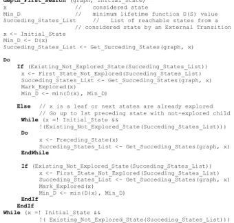
For that purpose, we defined an algorithm that ex-plores, from a considered state, the graph of reach-able states in order to compute a state relative looka-head. In Fig. 3, we present a pseudo-code algorithm of this solution that is based on oriented graphs clas-sical depth-first search algorithm.
We use the list of adjacencies of a considered node of the graph to obtain the
Succed-ing_States_List. This algorithm computes the relative
Lookahead for an Initial_State, which is equal to
Min_D at the end of the graph exploration (i.e. Min_D
is the min D(S) of reachable states).
Let us focus on Fig. 4 that represents a simple DEVS atomic model (i.e. a G-DEVS model of 0 order) with the graphical representation of [17]. The discrete state of the models considered in this sub-section is defined only by the phase state variable (with values represented by circles). For that reason, a lifetime value can be associated to each phase value
(refer-enced by numbers inside circles). Solid arcs represent external transitions δext; for instance, mark “com?o1”
on an arc of this type describes that the model state will transit by receiving an input event of “o1” value on the input port “com”. Dotted arcs represent internal transitions δint; if it elapses lifetime length in the
source phase of this type of arc, mark “out!set” shows, for instance, that the model state will transit and emit an output event of “set” value on output port “out”. Tri-angles represent input and output ports.
depth_First_Search (graph, Initial_State) x // considered state
Min_D // minimum lifetime function D(S) value Succeding_States_List // List of reachable states from a
// considered state by an External Transition x <- Initial_State Min_D <- D(x) Succeding_States_List <- Get_Succeding_States(graph, x) Do If (Existing_Not_Explored_State(Succeding_States_List)) x <- First_State_Not_Explored(Succeding_States_List) Succeding_States_List <- Get_Succeding_States(graph, x) Mark_Explored(x)
Min_D <- min(D(x), Min_D)
Else // x is a leaf or next states are already explored // Go up to 1st preceding state with not-explored child While (x =! Initial_State &&
!(Existing_Not_Explored_State(Succeding_States_List))) Do x <- Preceding_State(x) Succeding_States_List <- Get_Succeding_States(graph, x) EndWhile If (Existing_Not_Explored_State(Succeding_States_List)) x <- First_State_Not_Explored(Succeding_States_List) Succeding_States_List <- Get_Succeding_States(graph, x) Mark_Explored(x)
Min_D <- min(D(x), Min_D) EndIf
EndIf
While (x =! Initial_State &&
!( Existing_Not_Explored_State(Succeding_States_List)))
Figure 3. G-DEVS model current state relative lookahead
If we consider an absolute lookahead not depend-ing on the current state, the lookahead of the Fig. 4 example is equal to one time unit. If B state is the cur-rent state of the example, considering the curcur-rent state relative lookahead, the lookahead can be in-creased to five times units (Fig. 4. minimum lifetime of not shadowed states). Moreover, the computation of all lookahead values is done before run time and so does not affect simulation performance.
A ∞ C 10 D 9 E1 F 8 H 5 ∞I com?o1 COMMANDE “com” “stop” “out” com?o2 com?o3 stop?1 com?o1 com?o1 stop?1 com?o1 com?o1 out!set out!set out!set out!set out!set J 6 G 7 B 10 Speci al Issue 1 Speci al Issue 1
7
S
IMULATION
N
EWS
E
UROPE
Speci
al Issue 1
The restriction of the computation presented in this sub-section comes from the fact that it can only be applied to models with D(S) functions depending on only one state variable called the phase. Because DEVS/G-DEVS formalism can express more complex models, we propose in the next sub-section to gener-alise this computation for models with D(S) function depending on several state variables.
4.4 Second G-DEVS/HLA Lookahead computation im-provement
In the following, we define an extension of the compu-tation of the lookahead in order to consider G-DEVS models with state defined by (2).
S = Q × (An+1) (2)
Where:
Q: (phase, sigma, Bn) where sigma is the lifetime
function D(S) of the current state, phase is a state variable with symbolic values and Bn (b
0,..., bn) is a
(n)-tuple set of discrete state variables. An+1: state variables (a
0,..., an+1) stores the
(n+1)-tuple polynomial coefficients of the last external event occurred with A subset of real numbers or integers [7]. The phase defines explicit subset of state set, which allows representing graphically the DEVS/G-DEVS models as stated in [17] and recalled in 3.4.
The Bn n-tuple finite set of integer valued state variables completes the definition of the considered G-DEVS model state.
The values of the state variables are modified by the δext and δint transition functions. Note that we do
not consider the elapsed time in the current state to change the values of the next state.
Moreover, in the G-DEVS models considered, each lifetime is a mathematical function of D(phase, Bn), it does not depend on An+1 (e.g. Fig. 5 a).
4.4.1. Path search in G-DEVS models. The
looka-head is the minimum delay to emit an output event, which corresponds to the earliest next λ(s) among the reachable phase values by a sequence of δext.
Path search algorithms seem to be suited to ana-lyze the variation of state variables involved as pa-rameters of D(s), because the considered G-DEVS models can be represented by nodes/arcs. The only mismatch comes from classical graph path search al-gorithms only consider one variable (i.e. that is the path weight between two nodes) but G-DEVS models graphs can possess more than one state variable. In the considered model, there are n state variables B.
A key to this mismatch is to decompose a consid-ered G-DEVS model (e.g., Fig. 5 a) into as many
sub-models as the model contains state variables B. From each sub-model with S = ((phase, sigma, B), An+1), we create an oriented graph by representing the phase values of the G-DEVS model as nodes and the δext as
edges (e.g. Fig. 5 b,c,d).
The edges of a G-DEVS sub-model are weighted by the part of the δext function that handles the
con-sidered B state variable. Therefore, it implies that the state variables of Bn are independent in the
expres-sion of δext (i.e. each B variable must only be
depend-ent on constant values or on itself in the δext
func-tions). We can apply on the obtained oriented graphs a path search algorithm to track the variations of state variable B.
4.4.2. Dijkstra path search. Considering an oriented
graph (obtained from a G-DEVS sub-model) and the phase value phasei, we define a function (3), which
computes the shortest path (in terms of a considered bj of Bn) to reach each other phasek by a sequence of
δext.
ShortestPath(phasei, bj, phasek) = min bj in phasek (3) / considering an initial value of bj in phasei and k ∈ reachable phase value list of phasei
For example in Fig. 5 b), the shortest path from phase A to the others phase values, considering state variable b1, is 10 for reaching phase B, 2 for C, 10 for D and not defined for E because it is not linked from A
by external transition.
To implement the ShortestPath function, we ap-plied the Dijkstra Algorithm [3] that fulfils requirements of the function. The limitation is that this algorithm is not suited for graphs that contain circuits with edges of negative weight; indeed the looping of such circuits decreases iteratively the weight of the path. As a re-sult, the considered G-DEVS models must contain only B variables defined on R+ and δext functions that
only increment the state variables of Bn. We notice that others algorithms (e.g. Warshall and Floyd) allow the use of negative weight edges but the studied graphs still must no contain negative weight circuit.
We use the modified Dijkstra Algorithm (by chang-ing the values searched from min to Max) to find the longest path from a considered phase value to all oth-ers. This search computes the state variable B maxi-mal values for each reachable phase value. It implies a restriction on graphs type; it can be applied only to acyclic graphs (i.e. without circuits) because finding the longest path in a cyclic graph has been shown to be an NP-hard problem. Notice that cyclic graphs can be considered only if all state lifetimes D(s) contain no decreasing part since we do not search for the maxi-mum of the state variables.
S
IMULATION
N
EWS
E
UROPE
Speci
al Issue 1
Speci
al Issue 1
4.4.3. State lifetime D(s) analysis. Using min/Max
values of state variables of Bn (obtained from short-est/longest path computation), we exploit mathemati-cal backgrounds to study the variations of state life-time D(s). We consider D(s) as real-valued functions of several variables. The functions must be continu-ous, defined and derivable in all points of the state variables values range in order to determine their minimal value regarding to min/Max values of the state variables of Bn. To respect these definitions, we bound the study to linear state lifetimes D(s) defined by independents state variables (i.e. a linear function of several variables b1, b2, ... , bn is described by (4)).
f(b1, b2, ..., bn) = α0 + α1b1 + ... + αnbn (4) / {α0, ..., αn} are constants real values.
Taking into account the restrictions on state life-time D(s), we can compute a minimum value of state lifetime of a reachable phase value from a considered one regarding to min/Max values of the state vari-ables. More formally, for a phase value phasek and
the state variables b1, ..., bn, the state lifetime is
de-fined by (5).
D((phasek, sigma, Bn), An+1) = α0 + α1b1 + ... + αnbn (5) if αi < 0 we consider maximum value of bi / i ∈ {0,…, n} if αi ≥ 0 we consider minimum value of bi / i ∈ {0,…, n}
By repeating this computation for each reachable phasek from a considered phasei, we calculate the
lookahead (6) of the considered phase value equal to the minimum of all the reachable phase value state lifetime D(s) (we do not consider sigma and An+1).
Lookahead (phasei) = min D(phasek, min/Max (Bn)) (6)
∀ k ∈ reachable phase value list of phasei
If some G-DEVS models federates in a G-DEVS coupled model federation do not respect the restric-tion on state lifetime D(s) and on the state variables variations or if state lifetime D(s) computation con-cludes to a negative value result, then no minimum of state lifetime D(s) can be computed. We set, in that case, the lookahead of these G-DEVS model feder-ates equal to a minimum value ε negligible regarding to values taken by state lifetime D(s). Thereby, the simulation is constrained and slowed, by the looka-head of this federate.
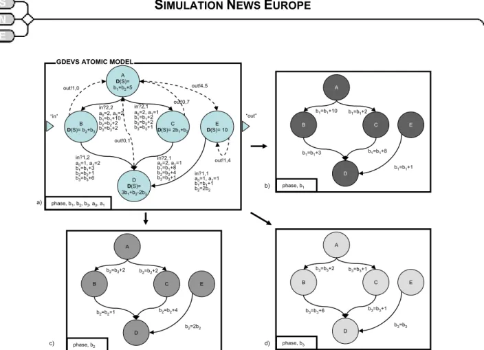
4.4.4. Lookahead computation example. Fig. 5 a)
example is an order 1 G-DEVS model. We consider an initial state with phase=A and b1=b2=b3=a0=a1=0.
We focus on the computation of the lookahead of phase A. As a result, we determine the reachable phase values from A by a sequence of external transi-tions that are B, C, and D. The state lifetime D(s) val-ues of these phase valval-ues are dependent on the ex-ternal transition passed from A to attain the consid-ered phase value.
For instance, state lifetime D(S) of phase D is equal to 3b1+b2-2b3. It implies to consider the
mini-mum value of b1 and b2 and the maximum value of b3.
Djikstra algorithms find out the extremes values of the state variables for each phase value.
We focus first on the sub-model represented in Fig. 5 graph b) that only considers the phase and b1.
From the initial state, we compute that b1 minimum
value is 10 time units in phase B, 2 for C, 10 for D and not defined for E.
By repeating the same process, we compute b2
minimum, values in Fig. 5 graph c). The min of b2 is 2
for B, 2 for C, 3 for D and not defined for E.
In Fig. 5 graph d): b3 minimum is 2 for B, 1 for C, 2
for D and not defined for E.
Because the D(s) function of phase D contains a subtraction, it is necessary to compute b3 maximum
value in Fig. 5 graph d) that is equal to 8 for D. Using these values, we compute the minimum val-ues of the D(s) functions for each reachable phase value from A:
min D(A, min/Max (Bn)) = b
1 + b2 + 5 = 0 + 0 + 5 = 5 min D(B, min/Max (Bn)) = b 2 + b3 = 2 + 2 = 4 min D(C, min/Max (Bn)) = 2b 1 + b2 = 4 + 2 = 6 min D(D, min/Max (Bn)) = 3b 1 + b2 - 2b3 = 30 + 3 – 16 = 17
The lookahead of phase A is equal to the minimum
D(s) of all reachable phase values. It is thus set, to 4
time units.
Using the same approach, we can compute the HLA lookahead for all phase values of the model. The lookahead is employed in the communication algo-rithm defined in [18] and recalled Fig. 2.
The limitation of this solution comes from its non-generic capabilities to handle all DEVS formalised models. In more details, this improvement does not allow to extend the lookahead computation to all kinds of DEVS/G-DEVS models; e.g. models with non-explicit phase, state variables defined on R and non linear D(s) functions are not considered in this study.
9
S
IMULATION
N
EWS
E
UROPE
“out” “in” out!0,1 phase, b1, b2, b3, a0, a1 B D(S)= b2+b3 D(S)= 2bC 1+b2 D D(S)= 3b1+b2-2b3 E D(S)= 10 in?2,2 a0=2, a1=2 b1=b1+10 b2=b2+2 b3=b3+2 out!4,5 out!0,7 out!1,0 out!1,4 in?1,2 a0=1, a1=2 b1=b1+3 b2=b2+1 b3=b3+6 in?2,1 a0=2, a1=1 b1=b1+8 b2=b2+4 b3=b3+1 in?2,1 a0=2, a1=1 b1=b1+2 b2=b2+2 b3=b3+1 in?1,1 a0=1, a1=1 b1=b1+1 b2=2b2
GDEVS ATOMIC MODEL
A D(S)= b1+b2+5 phase, b2 B C D E b2=b2+2 b2=b2+1 b2=b2+4 b2=b2+2 b2=2b2 A b) a) c) d) phase, b1 B C D E b1=b1+10 b1=b1+3 b1=b1+8 b1=b1+2 b1=b1+1 A phase, b3 B C D E b3=b3+2 b3=b3+6 b3=b3+1 b3=b3+1 b3=b3 A
Figure 5. Lookahead computing in G-DEVS model with complex lifetime function
5. Simulation results
We have implemented the algorithm of Fig. 2 on two distributed Pentium 4-based computers with 2.4 GHz, 256 Mo RAM, Windows XP OS, interconnected by a 10 Mbps LAN. We ran G-DEVS coupled models federations, of 2, 4, 6 and 8 G-DEVS federates dis-tributed on the two computers, in order to measure the influence of the lookahead value on the execution time. In the tests, each federate contained a G-DEVS atomic model and published/subscribed to coupling HLA interactions to define the federation as a “closed-chain” of coupled model federates. The code was de-veloped in Java and the RTI (running on a third similar computer of the LAN) was the pRTI1516 of Pitch.
0 10 20 30 40 50 60 70 80 90 100 110 2 4 6 8
Num ber of G-DEVS Federates
E xe cu ti on Ti me ( se cond ) Lookahead min 1/2 Lookahead Lookahead Max Speci al Issue 1
Figure 6. Execution time versus Lookahead value
The Fig. 6 shows that G-DEVS federation execu-tion is speeded up using a maximum lookahead (com-puted from the lifetime of the G-DEVS models phase as presented in 4.3 and 4.4). This assertion is done regarding the run time of the same federates models with half-reduced lookahead (representing the first so-lution proposed in 4.2 with a unique lookahead) and with negligible (min) lookahead (representing the pre-vious solutions recalled in 3.2).
The experiment also deduces that the speedup is nearly linear in number of federates. Thus, federates with a negligible lookahead value always produce an important overhead regarding federates with a maxi-mal lookahead. This overhead increases with the fed-eration size and appears clearly in Fig. 6 to slow sig-nificantly the simulation as stated theoretically.
6. Future work
The lookahead computation algorithm is still under the scope of our studies.
We are working on the improvement of this com-putation, particularly in the case of computing a long-est path. Because computing the longlong-est path is re-strictive on the class of G-DEVS models that can be handled, we try to compute it using algorithms of es-timate for the longest path proposed in the literature.
S
IMULATION
N
EWS
E
UROPE
Speci
al Issue 1
Speci
al Issue 1
We are also studying other kind of state lifetime
D(s) functions to be considered (e.g. real valued of
several variables interaction functions, distance func-tions, constrained functions).
7. Conclusions
In this article, we have presented a new HLA loo-kahead computing algorithm for distributed G-DEVS/DEVS models that uses the Dijkstra path search in a graph. It considers G-DEVS models with explicit phase and D(s) depending on several state variables instead of previous solutions that were con-sidering DEVS models with D(s) depending only on one state variable. In addition, a benchmark experi-ment has been performed to confirm the speedup of the G-DEVS federation execution due to the new loo-kahead computation.
Finally, this improvement extends the class of G-DEVS models that can be involved in a G-G-DEVS fed-eration. These models can be, more generally, cou-pled with heterogeneous HLA-compliant programs that respect, of their sides, the distributed time man-agement constraints and the event exchanged format.
References
[1] Bryant R. E., “Simulation of packet communication architecture computer systems”, Technical Report MIT/LCS/TR-188, MIT, 1977.
[2] Chandy K. M. and J. Misra, “Distributed simula-tion: A case study in design and verification of distrib-uted programs”, IEEE Transactions on Software Engi-neering, 5(5):440-452, September 1979.
[3] Dijkstra E.W., “A note on two problems in connex-ion with graphs”, Numerische Mathematik, 1:269-271, 1959.
[4] Fujimoto R. M., “Zero lookahead and repeatability in the high level architecture”, In Spring Simulation Interoperability Workshop (SIW), number 97S-SIW-046, Orlando, FL, 1997.
[5] Fujimoto R. M., “Time management in the high level architecture”, Simulation, 71(6):388-400, 1998. [6] Fujimoto R. M., Parallel discrete event simulation, Wiley Interscience, New York, NY, January, 2000. [7] Giambiasi N., B. Escude and S. Ghosh, “G-DEVS A Generalized Discrete Event Specification for Accu-rate Modeling of Dynamic Systems”, Transactions of the Society for Computer Simulation International, 17(3):120-134, 2000.
[8] Glinsky E., G. A. Wainer: “DEVStone: a Bench-marking Technique for Studying Performance of DEVS Modeling and Simulation Environments”. DS-RT 2005: 265-272, Montreal CA, 2005.
[9] IEEE std 1516-2000. IEEE Standard for Modeling and Simulation (M&S) High Level Architecture (HLA) - Framework and Rules. IEEE, NY, NY, USA, 2001. [10] IEEE std 1516.1-2000. IEEE Standard for Model-ing and Simulation (M&S) High Level Architecture
(HLA) - Object Model Template (OMT) Specification. IEEE, NY, NY, USA, 2001.
[11] IEEE std 1516.2-2000. IEEE Standard for Model-ing and Simulation (M&S) High Level Architecture (HLA) - Federate Interface Specification. IEEE, NY, NY, USA, 2001.
[12] Jefferson D.R., “Virtual Time”. ACM Trans. Prog. Lang. and Syst. 7(3):404-425, 1985.
[13] Kim K., W. Kang, B. Sagong, H. Seo, Yeungnam University “Efficient Distributed Simulation of Hierar-chical DEVS Models: Transforming Model Structure into a Non-Hierarchical One” 33rd ASS, 2000 Wash-ington, D.C. p. 227, 2000.
[14] Lake T., B.P. Zeigler, H.S. Sarjoughian and J. Nu-taro, “DEVS Simulation and HLA Lookahead” In Simu-lation Interoperability Workshop (SIW), number 00S-SIW-160, Orlando, FL, 2000.
[15] Lamport L., “Time, clocks and the ordering of events in a distributed system”. Communication of the ACM, 21(7):558-565, July 1978.
[16] Straßburger S., “Overview about the High Level Architecture for Modelling and Simulation and Recent Developments”. SNE special Issue 1 "Parallel and Distributed Simulation Methods and Environments", july-Aug 2006.
[17] Song H.S. and T.G. Kim, “The DEVS framework for discrete event systems control”, In 5th Conference on AI, Simulation and Planning in High Autonomous Systems:228-234, Gainesville, USA, 1994.
[18] Zacharewicz G., N. Giambiasi and C. Frydman, “Improving the DEVS/HLA Environment”, In DEVS In-tegrative M&S Symposium, DEVS'05, Part of the 2005 SCS Spring Simulation Multiconference, Spring-Sim'05, San Diego, CA, USA, April 3-7 2005.
[19] Zacharewicz G., N. Giambiasi and C. Frydman, “A New Algorithm for the HLA Lookahead Computing in the DEVS/HLA Environment”, In SISO European Simulation Interoperability Workshop (EUROSIW), number 05E-SIW-028, Toulouse, France, 2005. [20] Zeigler B.P. and J.S. Lee, “Theory of quantized systems: formal basis for DEVS/HLA distributed simu-lation environment”, SPIE, 3369 (Enabling Technology for Simulation Science II):49-58, A.F. Sisti Ed, 1998 [21] Zeigler B.P., G. Ball, and al, “The DEVS/HLA Dis-tributed Simulation Environment And Its Support for Predictive Filtering”, Technical Report Dept., DARPA Contract N6133997K-0007, UA, Tucson, AZ, 1998. [22] Zeigler B.P., G. Ball, H.J. Cho and J.S. Lee, “Im-plementation of the DEVS formalism over the HLA/RTI: Problems and solutions”, In Simulation In-teroperation Workshop (SIW), number 99S-SIW-065, Orlando, FL, 1999.
[23] Zeigler B.P., H. Praehofer and T.G. Kim, Theory of Modeling and Simulation, 2nd Edition, Academic Press, New York, NY, 2000.