Search for the Higgs boson decay into a pair of taus in ATLAS

(1)

HAL Id: tel-01253915

https://tel.archives-ouvertes.fr/tel-01253915

Submitted on 11 Jan 2016

HAL is a multi-disciplinary open access

archive for the deposit and dissemination of sci-entific research documents, whether they are pub-lished or not. The documents may come from teaching and research institutions in France or abroad, or from public or private research centers.

L’archive ouverte pluridisciplinaire HAL, est destinée au dépôt et à la diffusion de documents scientifiques de niveau recherche, publiés ou non, émanant des établissements d’enseignement et de recherche français ou étrangers, des laboratoires publics ou privés.

Search for the Higgs boson decay into a pair of taus in

ATLAS

Faten Hariri

To cite this version:

Faten Hariri. Search for the Higgs boson decay into a pair of taus in ATLAS. High Energy Physics -Experiment [hep-ex]. Université Paris-Saclay, 2015. English. �NNT : 2015SACLS065�. �tel-01253915�

(2)

(3)

c

(4)

Search for the Higgs boson decay into a pair of taus in ATLAS

by

Faten Hariri

Submitted to the Université Paris-Saclay on October 30, 2015, in partial fulfillment of the

requirements for the degree of Doctor of Philosophy of Science (Physics)

Abstract

Keywords: ATLAS, Higgs boson, tau lepton, missing transverse energy, Higgs effective field theory (HEFT)

In the LHC project, one of the major goals was the search for the last missing piece of the standard model (SM), namely the Higgs boson (H). The quest was successful during the Run I data taking in 2012 with the discovery of a new scalar of mass_∼125 GeV, compatible with the SM Higgs boson, and decaying to two bosons (either two photons or two electroweak vector bosons ZZ or 𝑊+_𝑊−

). To complete the picture, one needed to establish the couplings of the new particle to fermions. This motivated the search for the decay mode into two tau leptons predicted with a high branching ratio.

Inside the ATLAS collaboration, the analysis was divided into three channels accord-ing to the decay modes of the tau pair. The work reported in this Ph.D describes the ‘lepton-hadron’ analysis where one tau lepton decays leptonically into an electron or a muon and the other decays hadronically. Common features of all three analyses are the identification of the hadronic tau lepton and the presence of large missing transverse energy (MET) due to the escaping neutrinos from the tau decays.

An important contribution reported in this dissertation concerns the improvement brought by a new MET determination. By using charged tracks to estimate the con-tribution of the soft energy component produced in the proton-proton collision, the sensitivity to the overlaid events (‘pile-up’), unavoidable in a high luminosity hadron collider, is very much reduced. The systematic uncertainties associated to this soft component were estimated, their dependence on physics modeling and pile-up con-ditions studied for various track MET definitions. It will contribute to an improved 𝐻 → 𝜏+_𝜏−_{analysis with future data. In the lepton-hadron H analysis, the dominant}

background comes from events where a hadronic jet is misidentified as a hadronic tau (‘fake-tau’). The work reports in detail how this fake-tau background has been estimated in the two most sensitive event configurations predicted for the H signal i.e. events where the H boson is highly boosted or where it is produced by fusion

(5)

of vector bosons (VBF); VBF events are characterized by two forward and backward jets in addition to the H decay products.

Finally, the thesis reports on a last contribution performed with the Higgs Effec-tive Field Theory (HEFT) to study the H couplings and probe new physics beyond SM in a model independent way. The work consisted in testing and validating the ‘TauDecay’ model in association with the Higgs characterization framework in Mad-graph5_aM@NLO. After fixing some encountered problems and implementing a tool to merge H production and decay in a single step (especially useful with NLO re-quirements), the validation was done in three different ways: direct matrix element generation, with the implemented merging tool and using MadSpin to decay taus. The combined package is ready for use in the LHC Run II context.

Résumé

Titre: Recherche de la désintégration du boson de Higgs en deux leptons taus dans l’expérience ATLAS

Mots clés: ATLAS, boson Higgs, lepton tau, énergie transverse manquante, théorie effective des champs (HEFT)

Au LHC, l’un des buts essentiels était de trouver la dernière pièce manquante du modèle standard (MS), i.e. le boson de Higgs (H). La recherche fut couronnée de succès avec les données prises en 2012 et la découverte d’une nouvelle particule scalaire de masse _{∼125 GeV se désintégrant en deux bosons (deux photons ou deux} bosons électrofaibles ZZ or 𝑊+_𝑊−_{). Pour vérifier la compatibilité de la nouvelle}

particule avec les prédictions du MS, son couplage aux fermions devait être établi, ce qui motiva la recherche du Higgs dans le mode de désintégration en deux leptons taus ayant un rapport d’embranchement important.

Dans ATLAS, cette analyse est divisée en trois canaux selon le mode de désin-tégration des leptons taus. Le travail présenté dans cette thèse concerne le canal ‘lepton-hadron’, où l’un des taus de l’état final se désintègre leptoniquement en un muon ou un électron, alors que l’autre se désintègre hadroniquement. Les canaux de l’analyse H_{→tau tau sont caractérisés par de larges valeurs de l’énergie transverse} manquante (MET) dans l’état final et adoptent la même technique pour identifier le lepton tau.

(6)

Dans cette thèse, une contribution importante, mettant en relief l’amélioration obtenue avec une nouvelle estimation de MET, est montrée. En utilisant les traces chargées pour estimer la composante ‘molle’ de MET dans les événements issus de collisions p-p, la sensibilité à l’empilement (pile-up), inévitable dans les collisionneurs hadroniques à haute luminosité, est bien réduite. Les erreurs systématiques associées à la composante molle ont été évaluées et leur dépendance sur les conditions de pile-up et de modélisation de l’événement a été étudiée pour différentes définitions de MET. Ceci contribuera à améliorer les futures analyses H_{→tau tau.}

Dans l’analyse ‘lepton-hadron’, le bruit de fond dominant provient des événements dont un jet de hadrons est mal identifié comme un tau se désintégrant hadronique-ment (‘fake tau’). Le travail discuté montre en détail l’estimation de ce bruit de fond pour les deux configurations les plus sensibles aux événements de signal H, i.e. les événements produits avec un Higgs bien boosté ou ceux produits par fusion de deux bosons vecteurs (mode VBF). L’état final de ces derniers est caractérisé par deux jets bien séparés en pseudorapidité, répartis sur les deux hémisphères, produits en association avec les produits de désintégration du H.

Enfin, cette thèse rapporte une dernière contribution utilisant la théorie effective des champs pour estimer la production du boson de Higgs et ses couplages aux par-ticules du MS (HEFT), et explorer la nouvelle physique au delà du MS de façon indépendante du modèle théorique. Le travail consiste à tester et valider le mod-èle ‘tauDecay’ dans le cadre d’une caractérisation du Higgs utilisant HEFT au sein de Madgraph5_aMC@NLO. Après avoir écrit un outil permettant de fusionner les fichiers de production et de désintégration du Higgs (utile surtout en travaillant avec une précision au niveau NLO), la validation du modèle a été faite de 3 façons indépen-dantes: avec la génération d’événements au niveau d’éléments de matrice directement, avec l’outil créé et en désintégrant les taus avec MadSpin. Ce nouvel outil est prêt à être utilisé durant le Run-II du LHC.

(7)

(8)

Acknowledgements

First, I would like to express my sincere gratitude to the best supervisor ever, Michel Jaffré. Thanks for all the good times, the enjoyable discussions and for sharing your great knowledge with me. Thank you for believing in me, for encouraging and sup-porting me and for being there for me. You are a great friend. Without you, this journey would not have been possible.

My sincere thanks go to our group leader, David Rousseau, for his endless support on so many levels. You are a true friend and a leader like no other. Thank you for all the good moments we shared together, for all the excellent physics discussions, and for taking care of me like your own student. I could not have made it without you. I am very grateful to Achille Stocchi and Fabien Cavalier. Thank you for being there for me, for believing in me and supporting me. Special thanks to you, Achille, for your faith in me from the moment I was your student. Without you, this thesis would not have been materialized.

A big thank you to Francois LeDiberder for his great support and encouragement. With you, great opportunities are not a dream but a reality.

Many thanks to convenor Elias Coniavitis. Special thanks to exceptional con-venors Koji Nakamura and Teng-Jian Khoo for their help and support, and for all the great discussions.

A huge warm thank you to Fabio Maltoni for believing in me and giving me the opportunity to work with him and the great Madgraph5 team members. You are an excellent role model. Many thanks for the good discussions,for your guidance and for such a pleasurable working experience. Thanks to my good friend Pierre Artoisenet for his great help and support, for all the fruitful discussions and much more. Thank you Kentarou Mawatari for sharing your knowledge with me, your help and for all the good discussions. Thanks to my friends Federico and Ioannis for all the interesting discussions and help, and the memorable good times. Thanks to David, Eleni and Olivier. Thank you Ginette for being such a good, caring friend.

Many thanks to the MCnet community and to the network coordinator and project manager. Thank you for giving me this opportunity to be part of this great family.

Finally, last but most important, I would like to thank God for his great support and love, without which this work would have never been possible and this thesis would have never seen the light. I would also like to thank my dad for his

(9)

uncondi-tional love and support on so many countless levels. I am your student academically and in life. Thank you for all the things you’ve done for me. My love for physics grew through our discussions together and I became quite fond of particle physics thanks to you. Thank you for encouraging me to explore new fields and for your great pas-sion for science that I admire. Without you, I would not be who I am today. And I would like to thank my mom and sisters for their great love that knows no limits and for their great support. Thanks for being there for me throughout this journey. Without you, I would not have made it. You are the wind beneath my wings. You’re the reason I have come so far.

(10)

Author’s Contribution

I joined the ATLAS collaboration by the end of 2012 and started as an analyzer in the 𝐻 → 𝑊 𝑊* _{→ ℓ𝜈ℓ𝜈 analysis group, working on top background estimation and signal}

extraction. Then, I was ready to work on the search for Higgs in the 𝐻 _{→ 𝜏}ℓep𝜏ℎ𝑎𝑑

channel. In both channels, events are characterized by large missing transverse energy ‘MET’ in the final state, which also motivated the work on a promising pile-up ro-bust MET definition based on track measurements. After exploring the experimental aspects of the search for the Higgs boson in Run-I, I tried probing the spin/CP mea-surement in the 𝐻 → 𝜏+_𝜏− _{channel using the Higgs Effective Field Theory (HEFT)}

approach, which is now the default scheme for Run-II spin/CP studies. A summary of my contribution to ATLAS during my 2-year PhD work period is given below.

Track-based missing transverse energy

I was in charge of the evaluation of systematic uncertainties associated to soft terms of the track-based MET measurement ‘track MET’ (_{∼7 months) described in}chapter 5. My work includes :

– Evaluating the soft term systematic uncertainties for various MET definitions for both 2011 and 2012 data sets, and studying their dependence on MC gener-ators, pile-up, fast/slow simulation, event kinematics and potential correlations with the calorimeter based MET measurement. I wrote the systematics section of the track MET note :

F. Hariri, C. Lee, B. Liu, R. Mazini, and M. Testa, Measurement of track-based missing transverse momentum in proton-proton collisions at√𝑠 = 8 TeV centre-of-mass energy with the ATLAS detector, Tech. Rep. ATL-COM-PHYS-2013-1577, CERN, Geneva, Nov. 2013, https://cds.cern.ch/record/1645897/

– Implementing a user friendly tool for automatic systematics evaluation to be used by analysis groups.

Higgs Analyses:

𝐻

_{→ 𝑊 𝑊, 𝜏𝜏 channels}

∙ Work in 𝐻 → 𝜏𝜏 channel:

1. Based on the𝜏 -lepton decay modes (leptonic/hadronic), 3 orthogonal chan-nels are defined: lep-lep, lep-had and had-had. I worked on the lep-had channel, where the major background contribution from 𝑍 → 𝜏𝜏 sam-ples and from ‘fakes’, i.e. events with jets faking hadronic taus. I was in

(11)

charge of the evaluation of the fake tau background (fake factor method) and associated uncertainties for 7 TeV analysis, in addition to developing a functional analysis code and implementing the fake factor method in it. Results are explained in chapter 6. Additional details can be found in:

– Measurement of the Higgs boson couplings in the𝜏 𝜏 final state with the ATLAS detector - Supporting Note, https://cds.cern.ch/record/1666539 – Evidence for the Higgs-boson Yukawa coupling to tau leptons with the

ATLAS detector, JHEP 1504 (2015) 117

2. This work was followed by a study of track-based MET for global𝐻 → 𝜏𝜏 analysis to show the potential improvement in the lep-lep and lep-had channels as summarized inchapter 6 and explained in:

F. Hariri, Track MET for HSG4, HSG4 workshop, Orsay, June 2014, https://indico.cern.ch/event/324233/contribution/4/material/slides/1.pdf This is useful for Run-II analyses in particular since track-based MET is less pile-up dependent than the calorimeter based definition, while giving similar results especially for the final analysis distributions.

∙ Work in 𝐻 → 𝑊 𝑊 channel: I worked on optimizing the cut-based analysis used for Higgs signal extraction for both 2011 and 2012 analyses, and succeeded to improve the significance of the standard analysis of the ATLAS HWW group. Results are summarized in Appendix A.

HEFT and Monte Carlo tools

During my 4-month MCnet internship @UCLouvain with the Madgraph5_aMC@NLO team, I worked on the validation of the TauDecay model with the Higgs Character-ization (HC) framework, which uses a simple effective field Lagrangian (based on HEFT) below the EW symmetry breaking scale, yet is perfectly suitable to address questions on the strength of the Higgs coupling. The main advantage of HEFT is probing new physics in a model independent way while providing accurante spin/CP measurements. And the angular variables studied have a strong discriminating power regarding :

1. signal/background: 𝑍 _{→ 𝜏}+_𝜏− _vs _𝐻

→ 𝜏+_𝜏− _{(important for background}

re-duction in analysis) 2. 0±

spin hypotheses

which is promising for Run-II studies. In addition, a merging tool and an automation of a new MadSpin version were done as well as shown in chapter 7.

(12)

6.9.3 𝑍 _{→ 𝜏𝜏 Embedding . . . .} 210 6.10 Background Estimation . . . 214 6.10.1 𝑍 _{→ 𝜏𝜏 Background . . . .} 214 6.10.2 Fake Tau . . . 216 6.10.3 𝑊 +jets . . . 216 6.10.4 𝑍 _{→ ℓℓ +jets . . . .} 216 6.10.5 Top . . . 218 6.10.6 Diboson . . . 218 6.10.7 QCD . . . 218

6.11 Boosted Decision Trees . . . 218

6.12 Results and Systematic Uncertainties . . . 221

6.12.1 Systematic Uncertainties . . . 222

6.13 Track MET for 𝐻 → 𝜏+_𝜏− _{Analysis . . . .} ₂₂₉

7 Higgs Effective Field Theory and Tau Model Validation in Mad-graph5_aMC@NLO 239 7.1 Higgs Effective Field Theory (HEFT) . . . 239

7.1.1 Introduction . . . 239

7.1.2 Motivation . . . 240

7.1.3 Linear vs non-Linear Parametrization . . . 241

7.1.4 Building HEFT . . . 241

7.1.5 Effective Lagrangian: Basics . . . 242

7.1.6 HEFT Bases . . . 243

7.2 Importance of HEFT for LHC Run-II . . . 245

7.3 Higgs Properties (Spin/CP) and Monte Carlo Tools . . . 245

7.4 Higgs Characterization (HC) Framework . . . 246

7.4.1 HC Effective Lagrangian . . . 247

7.4.2 Comparison with JHU Results . . . 248

7.5 Application in Higgs Analyses . . . 252

(16)

7.7 Testing and Validation of HC+Tau Model in Madgraph5_aMC@NLO 253 7.8 Conclusions and Prospectives . . . 255

Conclusions and Prospectives 263

A Optimized 𝐻 → 𝑊+_𝑊− _{→ ℓ𝜈ℓ𝜈 analysis} ₂₆₅

A.1 Optimized 𝐻_{→ 𝑊 𝑊}* _{analysis with track MET . . . .} ₂₆₅

B Track MET for the 𝐻 _{→ 𝜏}+_𝜏−

analysis 279

C Résumé Substantiel 283

C.1 Track MET . . . 284 C.2 Analyse 𝐻 _{→ 𝜏}+_𝜏− _{. . . .} ₂₈₅

(17)

(18)

List of Figures

1-1 Summary of the SM particle content. . . 7 1-2 Scalar potential shape for 𝜇2 _{> 0 (left) and} _𝜇2 _{< 0 (right). In the}

latter, degenerate minima exist with different phases𝜃 [9]. . . 10 1-3 Summary of Higgs couplings to bosons and fermions in addition to

self-interaction terms [10]. . . 13 1-4 The 4 main Higgs production processes at LHC Run-I. . . 15 1-5 Cross section of the main Higgs production processes at LHC Run-I at

√

𝑠 = 8 TeV [14]. . . 15 1-6 Feynman diagrams illustrating the Higgs direct decay into a pair of

bosons (left) and fermions (right) at leading order. The𝐻 →γ γ decay is not shown as it is loop induced (see Fig. 1-7). . . 16 1-7 Leading-order Feynman diagrams showing the Higgs decay into a pair

of photonsγ γ. . . 16 1-8 Higgs branching ratios and their uncertainties for the low mass range

(left) and for the full mass range (right) [15]. The solid line in deep red for 𝑚𝐻 > 300 GeVis for the 𝑡𝑡 mode. . . 18

2-1 Plot showing the LHC design (a) [2] and the various stages of par-ticle acceleration at LHC (b) [5]. The energy values shown are for √

𝑠= 7 TeV in 2011. . . 24 2-2 Schematic representation showing the four major experiments and the

two ring structure of the LHC. Interaction points (IPs) are labelled based on octant. For example, ATLAS is at IP1 [9]. . . 27 2-3 Average number of interactions per crossing at LHC in 2011 (blue) and

2012 (green) [11]. . . 28 2-4 A graphical representation of the various parts of ATLAS detector

obtained by computer simulation [15]. . . 30 2-5 Layout of the ATLAS inner detector [14, 15]. The graphical

represen-tation in (b) does not include the additional Insertable B-Layer (IBL), which was added during the 2013-2014 shutdown after Run-I. . . 32 2-6 Figure showing where the IBL is inserted in the pixel detector [21]. . 33 2-7 Segmentation of the EM calorimeter barrel module in (𝜂, 𝜑) [14]. The

various parts of the EM LAr calorimeter are shown in (b)[15]. . . 40 2-8 Jet energy resolution as determined in situ and extracted from Monte

(19)

2-9 Graphical representation of the tile calorimeter layers [15] (a) and schematic drawing of the tile calorimeter mechanical structure and readout (b) [14]. . . 42 2-10 Evolution of the percentage of non-reconstructed tile calorimeter faulty

cells (masked cells) during Run-I 2011-2012 data taking period (left). The 2D-histogram (right) shows the (𝜂, 𝜑) positions of the masked cells at the end of 2012 [36]. The𝑧-axis shows the number of tile cells corresponding to each (𝜂, 𝜑) position. . . 43 2-11 Graphical representation of a HEC module (a) and the corresponding

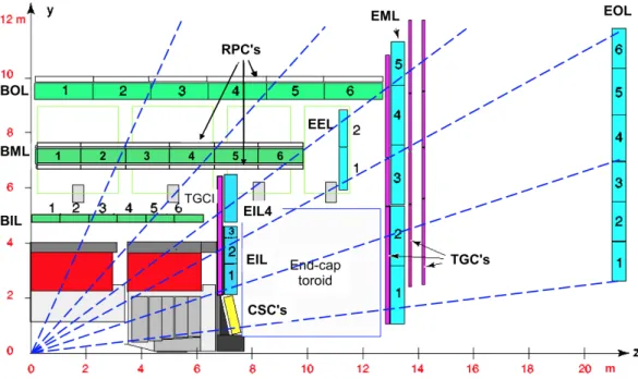
readout electronics (b) [14]. . . 44 2-12 Schematic representation of the ATLAS muon system in plane

contain-ing the beam axis (bendcontain-ing plane). Blue dashed lines show trajectories of muons with infinite momentum [14]. . . 46 2-13 Figure showing the definition of the sagitta ‘ s’ as the maximum

de-viation of the curved trajectory from a straight line. The definition is shown for 3-point trajectories, which is the case of muon tracks in ATLAS. L is the distance between the end points 1 and 3. . . 48 2-14 Schematic representation of trigger performance in ATLAS during 2012.

Design values are shown in addition to the actual peak values [40]. Items circled in red are the ones that need to be adjusted for Run-II requirements. . . 50 2-15 Figure showing trigger rates during 2012 data taking in Run-I [41]. . 50 2-16 Figure showing efficiency with respect to offline trigger for electrons

(a), muons (b) and jets (c) as a function of the transverse momentum [41]. . . 51 2-17 Figure showing trigger towers for e/𝛾 reconstruction [14]. . . 52 2-18 Graphical representation of the muon trigger [14]. High-𝑝T and low𝑝T

refer to the L1 muon trigger thresholds. . . 53 3-1 ATLAS software simulation flow starting with event generators (top

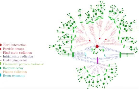
left) till reconstruction (top right) [1]. SDOs and RODs stand for Simulated Data Objects and Read Out Driver electronics during the dgitization step. . . 60 3-2 A graphical representation of the various event generation steps for a

𝑡¯𝑡𝐻 event [9]. . . 62 4-1 Track perigee parameters illustrated in the transverse𝑥-𝑦 plane (left)

and 𝑟-𝑧 plane (right) as defined in ATLAS. . . 70 4-2 Sketch illustrating track seed parameters [8]. . . 71 4-3 Normalized distributions showing track parameter resolution for track

seeds matched to the generated particles compared to those of the final tracks (final fit) in minimum bias MC simulation samples [8]. . . 75

(20)

4-4 Plot (a) shows the data and MC track candidates at different stages of the ambiguity solver for primary particles [8]. Plot (b) shows the pri-mary track reconstruction efficiency as a function of the pseudorapidity 𝜂 in minimum bias MC samples for two selections: default and robust requirements. Distributions are done for different pile-up conditions: no pile-up, average number of interactions_{⟨𝜇⟩ = 21, 41 [}19]. . . 76 4-5 2011 Data (closed markers) to MC samples (open markers) comparison

of the average number of tracks as a function of the number of inter-actions per beam crossing for both default (black) and robust (red) requirements is shown in (a). The dashed lines in (a) show the linear fit of the track multiplicity for tracks meeting the robust requirements. Plot (b) shows the transverse impact parameter 𝑑0 distributions for

tracks meeting the robust requirements in data for various pile-up con-ditions [19]. . . 77 4-6 Plot showing different vertex definitions. . . 78 4-7 Distribution of the reconstructed number of vertices in various pile-up

conditions (a) and the correlation with the average number of interac-tions per crossing [19, 20]. . . 78 4-8 (a) shows a qualitative fixed-size cluster representation for a single layer

in the EM calorimeter. The sliding window algorithm combines such clusters layer by layer. An example of a topo-cluster is shown in (b). 80 4-9 Resolution of the invariant mass from𝑍 → 𝑒𝑒 events after applying all

energy corrections in the 2011 data set. The fit shown in red uses a Breit-Wigner convoluted with a Crystal Ball function [15]. . . 87 4-10 GSF impact on the electron track resolution and impact parameter in

simulated MC events [16]. . . 91 4-11 Measured electron reconstruction efficiencies as a function of𝐸T integrated

over the entire pseudorapidity range in (a) and as a function of 𝜂 for 𝐸T between 10 and 50 GeV for 2011 and 2012 data sets [30]. . . 92

4-12 Measured electron reconstruction efficiencies as a function of the num-ber of primary vertices for 2012 data set is shown in (a). The combined reconstruction and identification efficiency as a function of 𝐸T is

plot-ted in (b) for cut-based loose, medium, tight and multilepton (They are mainly loose electrons with cuts on TRT variables used for Higgs_→ZZ channel) selections. (b) shows the statistical and systematic uncertain-ties on the measured efficiencies along with the data to MC efficiency ratio, useful for SF calculation, drawn in the bottom plot [30]. . . 93 4-13 Chain 1 muon reconstruction efficiency as a function of 𝜂 measured in

𝑍 _{→ 𝜇𝜇 events for various muon reconstruction types. This is done} for muons with 𝑝T > 10 GeV. CaloTag muons points are limited to

the region in 𝜂 where they are used in physics analyses. The CB + ST efficiency pile-up dependence is shown in (b) [33]. . . 94 4-14 ID muon reconstruction efficiency as a function 𝜂 (a) and 𝑝T (b) [33].

Pure statistical uncertainties are in green. Combined statistical and systematic uncertainties are shown in orange. . . 94

(21)

4-15 Muon isolation efficiency before (left) and after (right) pile-up correc-tions for 2011 data sets as done in𝐻 _{→ 𝑊 𝑊}* _{analysis for}_{Δ𝑅 = 0.3}

(top) and in𝐻 → 𝑍𝑍 analysis for Δ𝑅 = 0.2 (bottom) with Σ𝐸𝑇/𝑝 𝜇

𝑇 ≤ 0.14

[41]. . . 96 4-16 Resolution correction terms for the MS (a) and ID (b) muons. The

scale corrections for the MS and ID muons are shown in (c) and (d) respectively [26]. . . 98 4-17 Invariant mass distribution of Chain1 CB muons in 𝑍 → 𝜇𝜇 events

before (a) and after (b) applying scale and momentum smearing cor-rections [26]. . . 99 4-18 Invariant mass distribution of𝑍 → 𝜇𝜇 events with Chain 1 CB muons(a)

[33]. The signal muons are plotted along with the background events. Filled histograms are for MC samples with muon momentum correc-tions applied, while the dashed histogram shows the MC distribution without these corrections. Plot (b) shows data to MC Chain 1 CB di-muon mass ratio for 𝑍 _{→ 𝜇𝜇 (both muons with 𝑝}T > 25 GeVand

same𝜂 bin), 𝐽/Ψ→ 𝜇𝜇 (both muons with 𝑝T > 6 GeVand same𝜂 bin)

and ϒ_{→ 𝜇𝜇 (both muons with 𝑝}T > 6.5 GeV) events [26]. The 𝜂 of

the leading muon is shown. . . 100 4-19 Overview of the ATLAS jet reconstruction[37]. . . 101 4-20 Example of an event with random soft emissions at the parton-level

clustered into jets using anti-𝑘𝑇 algorithm with 𝑅 = 1[2]. . . 101

4-21 Data to MC response ratio for anti-𝑘𝑇 (R=0.4) LCW+JES jets in 2012

data as a function of the jet 𝑝T. The error bands show the statistical

uncertainties as well as the total (systematic and statistical uncertain-ties added in quadrature) uncertainuncertain-ties for three in-situ jet energy scale methods combined. The plot shows also the results for each method separately [23]. . . 103 4-22 JES fractional uncertainty at average pile-up conditions as a function

of the jet transverse momentum and pseudorapidity [25]. . . 104 4-23 The hard scatter jet efficiency using JVT and JVF for anti-𝑘𝑇 LCW+JES

jets (R = 0.4), with 20 < 𝑝T < 30 GeV and 30 < 𝑝T < 40 GeV, as

a function of the number of primary vertices in Pythia dijet samples [35]. The inclusive sample efficiency is 90%. . . 105 4-24 Normalized distribution of the median 𝑝𝑇 density 𝜌 for several values

of the number of primary vertices, 𝑁PV, for 20 <⟨𝜇⟩ < 21 [25]. . . . 106

4-25 A graphical representation of the jet vertex fraction JVF. . . 107 4-26 Graphical representation of secondary vertex reconstruction: 𝐿𝑥𝑦 is the

distance separating the secondary vertex from the primary vertex in the transverse plane, i.e. plane orthogonal to beam axis and 𝑑0 is the

track impact parameter in the transverse plane [40]. . . 108 4-27 MV1 algorithm light flavor rejection efficiency as a function of b-jet

tagging efficiency(a) [29]. The b-jet efficiency 𝑝T dependence is shown

(22)

4-28 (a): b-jet efficiency scale factors for MV1 b-tagging algorithm at 70% working efficiency in 𝑡¯𝑡 samples [28]. The green band shows total un-certainty (statistical+systematic). The scale factors to correct the ef-ficiency with which the b-tagging algorithms identifies c-jets is shown in (b) [29]. . . 110 4-29 Diagram showing hadronically decaying tau and QCD jet cones. . . . 110 4-30 Tau trigger rates for 2012 data as a function of the instantaneous

lu-minosity: Level-1 trigger L1(a) and Event Filter(EF) in (b) [32]. . . . 111 4-31 𝜏had-vis track efficiency as a function of the average number of

interac-tions per crossing for 1-prong taus in 𝑍 → 𝜏+_𝜏− _{events : the} _𝜏 had-vis

candidates are required to have 𝑝𝜏

𝑇 > 15 GeV and match truth-tau

within a distanceΔ𝑅 < 0.2. With TJVA, the efficiency is less pile-up sensitive with a small degradation at high pile-up values [21]. . . 112 4-32 Graphical representation of tau reconstruction steps summarized. . . 113 4-33 Normalized distributions of 𝑓cent in (a), 𝑁trackiso in (b) and 𝑅track in (c)

in both signal samples (𝑍, 𝑍′

→ 𝜏+_𝜏− _and _𝑊

→ 𝜏𝜈) and background samples obtained using 2012 data. The inverse background efficiency as a function of the signal efficiency is plotted in (d) [32]. . . 115 4-34 Distributions of 𝑓HT and 𝑓EM in simulated 𝑍 → 𝜏+𝜏− and 𝑍 →

𝑒𝑒 samples [32]. . . 116 4-35 Inverse background efficiency(𝑍 → 𝑒𝑒 ) as a function of the signal(𝑍 →

𝜏+_𝜏−

) efficiency for e-veto for various 𝜂 regions [32]. . . 117 4-36 Pseudorapidity 𝜂 (a) and 𝑓EM (b) normalized distributions in

recon-structed 𝜏had,vis matched to true muons and true taus. 𝜏had,vis

candi-dates overlapping with reconstructed muons are discarded [22]. . . 118 4-37 𝜏had-vis signal (top) and background (bottom) efficiency for 1-prong

(left) and 3-prong(right) taus for the different BDT working points for 2012 data, as a function of the true visible tau 𝑝T for signal and

reconstructed 𝑝T for background (QCD from data) [22]. . . 119

4-38 𝜏had-vis signal efficiency as a function of the number of the vertices in

the event for 1-prong (a) and 3-prong (b) taus [22]. . . 120 4-39 Tau SFs for all tau identification working points combined as a function

of 𝜂 for the muon and electron channels separately and together. The results are derived separately for 1-prong taus (a) and 3-prong taus (b) with𝑝T > 20 GeV. The error bars include combined statistical and

systematic uncertainties [32]. . . 120 4-40 𝐸miss

T distribution in 𝑍 → 𝜇𝜇 samples before (a) and after pile-up

suppression with MET-STVF (b) and MET-JetFiltered(c) [24]. . . 125 4-41 MET resolution as a function of the scalar sum of the measured physics

objects 𝐸T in the event, Σ𝐸𝑇, before and after pile-up suppression [24]. 126

4-42 𝐸miss

T linearity in ggF(gluon-gluon fusion) and VBF(vector boson

fu-sion) Higgs decaying in the 𝜏 𝜏 mode 𝐻 → 𝜏+_𝜏−_(𝑚

𝐻 = 125 GeV) (b)

as a function of the true 𝐸miss

(23)

5-1 Nominal Track MET distribution in Monte Carlo𝑍 _{→ 𝑒𝑒 events before} and after the removal of events with Bremsstrahlung electrons using a cut on electron 𝐸𝑇/𝑝𝑇 < 1.4, compared to 𝑍 → 𝜇+𝜇− results [1]. . . . 135

5-2 Resolutions of nominal calorimeter-based𝐸miss

T and jet corrected𝑝missT as

a function of the number of reconstructed vertices in the event𝑁PV (a)

and ∑︀ 𝐸𝑇. The resolution is improved when switching to the

track-based 𝑝miss

T estimation [1]. . . 137

5-3 Track 𝑝𝑇 distribution in 𝑍 → 𝑒𝑒 events from 2012 data before and

after mis-reconstructed track momentum rejection [1]. . . 140 5-4 Schematic representation of𝑝hard

T for the jet corrected definition (right)

and the remaining nominal and cluster definitions (left). For the latter, it is sometimes referred to as 𝑝Lep_T and the contribution from tracks associated to jets enters the soft term calculation. . . 142 5-5 Example showing the Gaussian fit of 𝑝miss

T,soft,L distribution, in a 𝑍 →

𝜇𝜇 data (at √𝑠 = 8 TeV) sample in the 1-jet bin, to extract the scale (mean) of 𝑝miss

T,soft . The results are derived for Track MET-Cl-j using

the ghost-association method in the first bin of phard

T , for events with

an average number of interactions per crossing_{⟨𝜇⟩ greater than 22. .} 143 5-6 Projection of𝑝miss

T,soft with respect to p hard,trk

T direction to extract𝑝missT,soft,L and

𝑝miss

T,soft,P. . . 144

5-7 Distribution of the average number of interactions per crossing _{⟨𝜇⟩ in} 𝑍 _{→ 𝜇𝜇 events at} √𝑠 = 7 TeV(left) and 8 TeV (right). The dashed lines show the limits defining the binning in _{⟨𝜇⟩ used for Track} MET-Cl-j calculations. . . 147 5-8 Scale and resolution results for Track MET-Cl in the inclusive 𝑍 _→

𝜇𝜇 samples. The scale uncertainty defined as the difference(shift) be-tween data and MC 𝑝miss

T,soft,L is plotted in the lower panel of (a). The

resolution uncertainty defined as the ratio of data to MC resolution values is plotted for 𝑝miss

T,soft,L and 𝑝 miss

T,soft,P in the lower panels of (b) and

(c) respectively. . . 149 5-9 Mean and resolution of𝑝miss

T,soft,L components of Track MET-Cl-j in𝑍 →

𝜇𝜇 0-jet(left) and inclusive(right) samples respectively using the Δ𝑅 method . . . 150 5-10 Mean and resolution of𝑝miss

𝜇𝜇 1-jet sample (bottom) and 𝑝miss

T,soft,P component(top) using the Δ𝑅

method. . . 151 5-11 𝑝hard

𝑇 distribution in 𝑍 → 𝜇𝜇 inclusive sample for Track

MET-Cl-j definition. The dotted lines show the binning limits as used for Track MET-Cl and the yellow dashed lines show the adjusted binning for the Track MET-Cl-j calculations. . . 152 5-12 Mean and resolution of𝑝miss

𝜇𝜇 0-jet(left) and inclusive(right) samples respectively using the Δ𝑅 method at √𝑠 = 7 TeV. . . 153

(24)

5-13 Mean and resolution of𝑝miss

𝜇𝜇 1-jet sample (bottom) and 𝑝miss

T,soft,P component(top) using the Δ𝑅

method at √𝑠 = 7 TeV. . . 154 5-14 Distributions of 𝑝miss

T,softvaried according to equation (5.7) are shown in

(a) along with the corresponding total 𝑝miss

T distributions (b) for the

𝑍 → 𝜇𝜇 inclusive sample. The results are derived for Track MET-Cl-j derived usingΔ𝑅 method at √𝑠 = 8 TeV. . . 155 5-15 Distributions of 𝑝miss

(a) along with the corresponding total 𝑝miss

T distributions (b) for the

𝑍 → 𝑒𝑒 inclusive sample. The results are derived for Track MET-Cl-j derived usingΔ𝑅 method at √𝑠 = 8 TeV. . . 155 5-16 ∑︀ 𝐸𝑇 comparisons for different pile-up conditions at √𝑠 = 8 TeV in

𝑍 → 𝜇𝜇 data and AlpgenHerwig simulated samples. The pile-up mod-eling is in fact studied in terms of the average number of interactions per crossing _{⟨𝜇⟩ (a) and of the number of reconstructed primary} ver-tices in the event 𝑁PV (b). . . 156

5-17 Distributions of (𝑝miss

T,soft,L ,∑︀ 𝐸𝑇soft term) in the inclusive (left) and 0-jet

bin (right) 𝑍 _{→ 𝜇𝜇 events. . . .} 156 5-18 Mean and resolution of 𝑝miss

T,soft,L component of Track MET-Cl-j in 𝑍 →

𝜇𝜇 inclusive (top) and 0-jet (bottom) samples. The results are derived for Track MET-Cl-j using the ghost association method. . . 160 5-19 Resolution of𝑝miss

T,soft,P component of Track MET-Cl-j in𝑍 → 𝜇𝜇 events

in the inclusive (left) and 0-jet bin(right). The mean and resolution of 𝑝miss

T,soft components of Track MET-Cl-j in 𝑍 → 𝜇𝜇 events in the 1-jet

bin are shown in the bottom plots. The results are derived for Track MET-Cl-j using the ghost association method. . . 161 5-20 Resolution of 𝑝miss

T,soft,P in 𝑍 → 𝜇𝜇 1-jet bin derived for Track

MET-Cl-j using the ghost association method. . . 162 5-21 Distributions of 𝑝miss

(a) along with the corresponding total𝑝miss

T distribution in (b) for the

𝑍 → 𝜇𝜇 inclusive sample. The results are derived for Track MET-Cl-j derived using the ghost association method. . . 162 5-22 Plot showing the difference between Track MET-Cl-j and the true

miss-ing transverse energy originatmiss-ing from the neutrino in simulated Alp-genPythia𝑊 → 𝜇𝜈 samples at √𝑠 = 8 TeV. . . 163 5-23 Effects of 𝑝hard

T component systematics on the measured𝑝missT,soft shift in

scale (mean) and resolution (smearing) for Track MET-Cl-j in 𝑍 _→ 𝜇𝜇 samples at √𝑠 = 8 TeV [10]. . . 164 5-24 Scale and resolution results for calorimeter based MET before pile-up

suppression in𝑍 _{→ 𝜇𝜇 data and AlpgenHerwig samples. . . .} 165 5-25 Scale results for calo MET before pileup suppression (top) and track

MET (bottom) for 𝑍 _{→ 𝜇𝜇 PowhegPythia8 (left) and Sherpa (right)} samples. . . 166 5-26 Resolution plots for calo MET (top) and Track MET-Cl (bottom) for

(25)

5-27 Resolution plots for calo MET (top) and Track MET-Cl (bottom) for 𝑍 _{→ 𝜇𝜇 events with Sherpa MC simulated samples. . . .} 168 5-28 MET-STVF definition (right) with an illustration of tracks coming

from primary (PV) and secondary vertices in an event (left). . . 170 5-29 𝑝miss

T,soft(left) and Σ𝐸𝑇 of soft term components (right) distributions for

various MET definitions for𝑍 _{→ 𝜏}+_𝜏− _{events in the}_𝐻

→ 𝜏+_𝜏−_analysis

lep-lep channel. . . 170 6-1 Figure showing a schematic representation of the angular separation

between the final state products and the MET vector, in signal and 𝑍 → 𝜏𝜏 lep-had events with additional jet(s) (left) and in 𝑊 +jets lep-had samples (right). . . 179 6-2 Figure showing normalized distributions of the signal and 𝑍 _{→ 𝜏𝜏 in}

the VBF signal region. . . 180 6-3 Figure showing an example of𝑍/𝐻 _{→ 𝜏}ℓ𝜏ℓ decays with collinear mass

approximation. The emitted tau decay products are collinear with the tau direction. The MET vector, assuming neutrinos are the only source of MET in the event, is illustrated as well. . . 181 6-4 Distribution of the Δ𝑅 separation between the neutrino(s) and the

visible tau decay products in simulated𝑍 → 𝜏𝜏 for hadronic 1-prong(a) and 3-prong(b), in addition to leptonic(c) tau decays for a chosen tau 𝑝𝑇 [3] . . . 183

6-5 Plots showing the probability distribution function of the 3-dimensional angular separation Δ𝜃3D between the neutrino(s) and the visible tau

decay products in simulated 𝑍 _{→ 𝜏𝜏 for hadronic 1-prong(a) and} 3-prong(b), in addition to leptonic(c) tau decays [5]. The results are shown for taus with a generated momentum 45 < p_{≤ 50 GeV. . . . .} 184 6-6 Normalized 𝑚MMC distribution in 𝑍 → 𝜏+𝜏− and 𝐻 → 𝜏+𝜏− lep-had

events for VBF and boosted analysis categories (defined in sec. 6.8) [2] .185 6-7 Figure showing normalized distributions of the transverse mass at the

preselection level for the signal and𝑊 +jets samples. . . 193 6-8 7 TeV FF values for boosted (top) and VBF(bottom) categories as

derived in each fake background type CR for 1-prong (left) and 3-prong(right) separately. . . 201 6-9 8 TeV FF values for VBF(bottom) and boosted (top) categories as

derived in each fake background type CR for 1-prong (left) and 3-prong(right) separately [60]. . . 202 6-10 Graphic representation of the fake tau background composition for

VBF 𝑍 _{→ 𝜏𝜏 CR (left) and SR (right) at 7 TeV. . . .} 204 6-11 Graphic representation of the fake tau background composition for

boosted𝑍 _{→ 𝜏𝜏 CR (left) and SR (right) at 7 TeV. . . .} 204 6-12 Effective FF value (FFmix) in the boosted (top) and VBF (bottom)

signal regions with systematic variations corresponding to the largest RX variation for 1-prong (left) and 3-prong (right) taus at 7 TeV. . . 205

(26)

6-13 Effective FF value (FFmix) in the boosted (top) and VBF (bottom) SR

for 1-prong (left) and 3-prong (right) taus at 8 TeV [60]. . . 206 6-14 Effective FF value (FFmix) in the boosted (up) and VBF (down)𝑍 →

𝜏 𝜏 CR for 1-prong (top) and 3-prong (right) taus at 7 TeV. . . 207 6-15 Fake background distribution for different FF statistical variations as

a function of𝑝𝜏

T for VBF(left) and boosted(right) events at 7 TeV. . . 208

6-16 Fake background distribution for different FF statistical variations as a function of event BDT score for VBF (left) and boosted (right) events at 7 TeV. The distribution is used for fake tau statistical uncertainty estimations. . . 209 6-17 Fake background distributions for FF up/down systematic variations

(see text) as a function of BDT score for VBF(left) and boosted(right) events at 7 TeV. . . 210 6-18 Closure plots showing fake tau distribution in𝑊 +jets CR in MC samples.211 6-19 Closure plots showing fake tau distribution in𝑍 _{→ ℓℓ CR in MC samples.}212 6-20 Closure plots showing fake tau distribution in top CR in MC samples. 213 6-21 FF values at 7 TeV as derived directly from MC simulation samples

except for QCD ones for VBF (left) and boosted (right). . . 214 6-22 Closure test in MC simulated samples boosted (left) and VBF(right)

SR at 7 TeV. . . 215 6-23 Closure test in MC simulated samples boosted SR (right) with MC

based MET correction weights (left) at 7 TeV. . . 215 6-24 Closure test in MC simulated samples boosted SR (right) with

data-based MET correction weights (left). . . 216 6-25 7 TeV closure test of the FF method performed in the MC signal region

for the boosted (left) and VBF (right) categories of the 𝜏ℓ𝜏had channel. 217

6-26 Closure test in fake tau SS CR for boosted (left) and VBF(right) SR at 7 TeV. . . 218 6-27 FF in the SS CR for VBF (left) and boosted (right) events for

both1-prong and 3-both1-prong taus at 7 TeV. . . 219 6-28 7 TeV closure test of the FF method performed in the SS data control

region for the boosted (left) and VBF (right) categories of the 𝜏ℓ𝜏had

channel. . . 220 6-29 Best-fit 𝜇 values per 𝐻 _{→ 𝜏}+_𝜏− _{channel and per analysis category}

(VBF, boosted). The green band shows the_{±1𝜎 uncertainty. The} con-tributions of statistical (black), theoretical (red) and non-theoretical (blue) systematic uncertainties are plotted separately [2]. . . 223 6-30 BDT score distributions for the various 𝐻 → 𝜏+_𝜏− _{channels, namely}

ℓℓ (top),ℓℎ (middle) and ℎℎ (bottom) at √𝑠 = 8 TeV. Post-fit results are shown for VBF (left) and boosted (right) signal regions with sta-tistical and systematic uncertainties. The background predictions as taken from the global fit (𝜇 = 1.4) are shown. And the data to model (background+Higgs signal prediction with strength 𝜇 ) ratio is shown in the lower panel of each plot for 𝜇 = 0.0 (solid black line), 𝜇 = 1.0 (dashed red line) and 𝜇 = 1.4 (solid red line) [2]. . . 226

(27)

6-31 Event yields as a function of log₁₀(𝑆/𝐵) for all channels combined (ℓℓ, ℓℎ, ℎℎ). The signal (S) and background (B) yields are estimated based on the BDT output bin of each event, with a signal strength 𝜇 = 1.4 hypothesis. All categories are taken into account. Back-ground events are displayed for the global fit (with 𝜇 = 1.4). Signal yields are shown for both 𝜇 = 1 and 𝜇 = 1.4 (the best-fit value) at 𝑚𝐻 = 125GeV. The dashed line corresponds to the background-only

distribution obtained from the global fit with𝜇 = 0 [2]. . . 227 6-32 𝑝miss

T,softandΣ𝐸𝑇Soft Termcomparison for different MET definitions in𝑍 →

𝜏 𝜏 (top), lep-had VBF (middle) and lep-lep VBF (bottom) samples. The comparison is done between MET STVF (black), jet corrected track MET TrkMETjet Corrected_𝑐ℓ (blue) and cluster Track MET (red). . . 232 6-33 Transverse mass distribution in VBF signal and 𝑍 → 𝜏+_𝜏− _events

in the lep-lep events with jet corrected track MET used as the MET definition entering the 𝑚𝑇 calculation. . . 233

7-1 Figure showing a 4-fermion effective vertex (left) in a 𝑒+_{𝑝 collision.}

The actual vertex with the W propagator is shown on the right. . . . 241 7-2 Figure showing the 5 angles fully characterizing the orientation of the

decay chain in pp _{→ 𝐻 → 𝑍𝑍 → 4ℓ}± events as used in the Mad-graph5_aMC@NLO plots. The angles are defined in the correspond-ing particle rest frame. The illustrated production and decay of a H particle are for various spin hypotheses, e.g. spin 0, spin 1 [34]. . . 249 7-3 Distributions of the X _{→ ZZ → 4ℓ analysis using the effective}

La-grangian as implemented in MG5 [34] for spin 0 (left), spin 1 (middle) and spin 2 (right) hypotheses. The Lagrangian parameter settings are shown on the plots. . . 250 7-4 Mass and angular distributions for the X _{→ WW analysis using the}

effective Lagrangian as implemented in MG5 [34] for spin 0 (left), spin 1 (middle) and spin 2 (right) hypotheses. . . 251 7-5 Angular distributions Φ = 𝜑1 + 𝜑2 and Δ𝜑 = 𝜑1 − 𝜑2 for events

produced directly at the matrix element (ME) level (top), obtained after merging X(𝐽𝑃_{) production and decay MG5 output (middle) and}

decayed with MadSpin (bottom). Plots are obtained with 100k events generated in Madgraph5_aMC@NLO. . . 256 7-6 The coordinate system in the tau decay frame [51]. . . 257 7-7 Invariant mass distributions with 10 000 events (no cuts applied) for

the𝑎1 and𝜌 tau decay modes in the 1-prong (a and b) and 3-prong (d)

topologies. The pion pair𝜋−_𝜋0 _and_𝜋−_𝜋+ _{invariant mass distributions}

for the 𝑎1 1-prong and 3-prong topologies are shown in (a) and (c)

respectively. . . 257 7-8 Angular distributions Φ = 𝜑1+ 𝜑2 and Δ𝜑 = 𝜑1− 𝜑2 obtained with

(28)

A-1 Graph showing the soft hadronic recoil (in gray) against the dilepton system (in yellow) used in the calculation of𝑓recoil for the Z/Drell-Yan

events. . . 267 A-2 Normalized distributions of 𝐸_T,Rel,Clmiss,track for the combined Higgs signal

and total background events in the 1-jet bin, illustrating how the Higgs phase space is closed in 𝐸_T,Rel,Clmiss,track with finite limits. The results are shown for the 2012 ℓ𝜈ℓ𝜈 analysis . . . 268 A-3 Plots showing significance for lower limit cut on 𝑝ℓℓ

𝑇 in the 0 jet bin

before (left) and after (right) applying an additional upper limit cut in the 2012 ℓ𝜈ℓ𝜈 analysis. . . 269 A-4 Normalized distributions of METRel (calorimeter-based MET) at

pre-selection for Higgs and background events in the SF (left) and OF (right) channels at the end of preselection in the 2012 ℓ𝜈ℓ𝜈 analysis. The pink lines show the limits taken into account during optimization for the definition of a METRel window cut. . . 271 A-5 Normalized Track METRel distributions for the Higgs and background

events in the 0 jet bin (top) and 1 jet bin (bottom) with optimized cut limits for the 2012ℓ𝜈ℓ𝜈 analysis. The pink lines show the limits taken into account during optimization for the definition of a track METRel window cut. . . 272 A-6 𝑝ℓℓ

𝑇 distribution in the 1-jet bin for all channels (OF+SF) combined in

the 2012 𝐻 → 𝑊 𝑊*_{ℓ𝜈ℓ𝜈 analysis. The pink lines show the proposed}

cut limits to improve the significance and enchance the obtained Higgs signal. . . 272 A-7 Distributions of 𝑝ℓℓ

𝑇 (left) and Track METRel (right) for events in the

0 jet bin kept in the ATLAS analysis but removed in the optimized analysis for the 2012 ℓ𝜈ℓ𝜈 analysis. . . 273 B-1 𝑝miss

various MET definitions for𝑍 _{→ 𝜏}+_𝜏− _{(top) and ggF(bottom) events}

in the lep-lep channel. . . 280 B-2 𝑝miss

various MET definitions for lep-lep VBF(top) and lep-had ggF (bot-tom) events. . . 281 B-3 𝑝miss

various MET definitions forVBF lep-had events . . . 282 B-4 𝑚MMC plots for gFF(left) and VBF(right) lep-had events . . . 282

(29)

(30)

List of Tables

1.1 Table giving a brief description of the SM symmetries. C and Y refer to the color quantum number and the hyper charge respectively. The suffix ‘𝐿’ in SU(2)𝐿 stands for left-handed, where weak interactions are

limited to left-handed fermions only. . . 6 1.2 Summary of the SM lepton generations and their basic properties [6].

𝐼3 refers to the weak isospin and the electric charge is given in units of

[e]. . . 6 1.3 Summary of the SM quark generations and their basic properties [6].

𝐼3 refers to the weak isospin and the electric charge is given in units of

[e]. . . 7 1.4 Table summarizing the basic properties of the SM gauge bosons and

the associated interactions [6]. . . 7 1.5 Relative parametric (PU) and theoretical (THU) uncertainties on the

SM Higgs partial widths for a selection of Higgs masses [15]. The PU are shown for each single parameter. . . 17 1.6 Table summarizing the signal strengths and statistical significance

val-ues in ATLAS for each Higgs search channel studied during Run-I at both√𝑠 = 7 and 8 TeV[19]. . . 19 2.1 Table showing 2012 beam parameters values justifying the choice of 50

ns bunch crossing over the design value of 25 ns [8]. . . 25 2.2 Table showing actual and design values of beam performance

parame-ters in 2012 [8]. . . 26 2.3 Table summarizing the track-to-hit pull widths before and after

scal-ing in addition to the correspondscal-ing C values for various parts of the ATLAS Inner detector [38]. . . 35 2.4 Table summarizing the measured values of the constant EM calorimeter

energy resolution term for various 𝜂 regions in ATLAS [30]. OW and IW stand for outer wheel and inner wheel in the end caps respectively. 38 2.5 The main parameters of the ATLAS muon system for both combined

and stand-alone performances [37]. . . 45 4.1 Table summarizing the values of tracking cuts of the inside-out

algo-rithm. (*) For full track reconstruction, selected tracks at the final stage are good tracks with at least 1 pixel hit [9, 12]. . . 73

(31)

4.2 Table showing qualitatively the effect of some track characteristics on the track score [39]. . . 74 4.3 EM Tower parametrization in the EM calorimeter barrel (EMB) and

end-cap (EMC) [42]. . . 80 4.4 𝜂_{− 𝜑 granularity of the three EM calorimeter layers [}4, 42]. . . 80 4.5 Cluster size definition for each EM calorimeter layer as used in the

slid-ing window algorithm. The layers are processed to build EM clusters in the order shown in the first column. The dimensions are expressed in tower bin units, i.e. in units of 0.025. 𝑁cluster

𝜂 and 𝑁𝜑cluster values

depend on the particle type hypothesis and on the region of the EM calorimeter. Their definitions for electrons and photons in the barrel and endcap are given in Table4.6 [42]. . . 82 4.6 Cluster size definition𝑁cluster

𝜂 × 𝑁𝜑clusterfor electrons and photons

(con-verted and uncon(con-verted) in the barrel and end-caps of the ATLAS EM calorimeter for the sliding window algorithm [42]. . . 82 4.7 𝜏had and QCD jet cone comparison. . . 108

4.8 Uncertainties on some basic tau performance measurements [32]. . . . 121 5.1 Comparison of the different contributions to soft and hard terms for

the different track MET definitions when evaluating systematic uncer-tainties in𝑍 _{→ 𝜇𝜇 samples. . . .} 141 6.1 Table showing the𝑚MMC efficiency for𝑍 → 𝜏𝜏 and Higgs signal events

for various mass hypotheses, in the ℓ𝜏had channel [5]. . . 184

6.2 Table summarizing the luminosity information for the 7 and 8 TeV data samples [6]. . . 186 6.3 Table summarizing simulated MC signal and background samples

in-formation at √𝑠 = 8 TeV. The last column states the order of the applied QCD corrections, in addition to showing the product of cross section by the corresponding branching ratio (𝜎_{× 𝐵) for each process,} except for those marked with a _{~. The latter are presented with the} corresponding inclusive cross section value in the last column [2]. . . . 187 6.4 Table summarizing physics object requirements when entering the

anal-ysis and at the preselection level. . . 190 6.5 Table summarizing preselection cuts in the lep-had channel . . . 191 6.6 Table summarizing the VBF and boosted categories signal region (SR)

and control regions (CRs) definitions. . . 194 6.7 Table showing the OS and SS normalization factors applied at the

preselection level for MC simulated samples at 7 TeV. . . 198 6.8 Table summarizing the contamination of the electroweak processes in

the QCD CR used for 𝑟QCD calculations [59]. . . 198

6.9 Fraction 𝑅𝑋 of the different fake background processes as derived in

(32)

6.10 Table showing variation of the fake tau composition fraction 𝑅𝑋 in the

range [𝑅𝑋/2, 𝑅𝑋 × 2] for systematic uncertainties evaluation in VBF

events at 7 TeV. . . 208 6.11 The most discriminating BDT variables for VBF and boosted

cate-gories listed in decreasing order of ranking [2]. . . 222 6.12 Post-fit event yields in the_√ 𝐻 → 𝜏ℓ𝜏had channel for 𝑚𝐻= 125 GeV at

𝑠 = 8 TeV. Background and signal normalizations are post-fit val-ues. Full statistical and systematic uncertainties are shown for the events under ‘Total background’ and ‘Total signal’. The individual background components uncertainties include the systematic uncer-tainties only [2]. . . 224 6.13 Table summarizing the expected and observed significances in various

𝐻 → 𝜏+_𝜏−

channel for both VBF and boosted categories[2]. . . 225 6.14 Most important sources of uncertainties affecting the signal strength

measurements. Results are shown for the best-fit 𝜇 value [2]. . . 225 6.15 Summary of fake tau background various uncertainties values at 7 and

8 TeV. . . 228 6.16 Systematic uncertainties post-fit for the signal𝑆 and the background 𝐵

for the 3𝐻 → 𝜏+_𝜏−

channels and for both VBF and boosted analysis categories at √𝑠 = 8 TeV. The correlation amongst channels is taken into account and the unaffected uncertainties are marked with a *. The ones with _{† have an important effect on the BDT distribution shape.} UE= underlying event and PS=parton shower [2]. . . 231 7.1 HC model parameters for the effective Lagrangian [40]. . . 248 A.1 Table summarizing the cut-based event selection at preselection and in

the 0- and 1-jet bin categories for the standard ATLAS Moriond 2013 for the 2012 𝐻 → 𝑊 𝑊*_{ℓ𝜈ℓ𝜈 analysis. . . .} ₂₇₄

A.2 Table summarizing the optimized cut-based event selection in the 0-jet bin category for the 2012𝐻 _{→ 𝑊 𝑊}*_{ℓ𝜈ℓ𝜈 analysis. The 𝑚}

𝑇 cut is not

shown since the final result of the cut-based analysis will be fitted for final signal extraction. . . 275 A.3 Table summarizing the optimized cut-based event selection in the 1-jet

bin category for the 2012𝐻 → 𝑊 𝑊*_{ℓ𝜈ℓ𝜈 analysis. The 𝑚}

𝑇 cut is not

shown since the final result of the cut-based analysis will be fitted for final signal extraction. . . 275 A.4 Table summarizing results of the optimized and standard ATLAS

anal-ysis (around Moriond 2013) for the 0 jet and 1 jet bin 2012 analanal-ysis. . 275 A.5 Table summarizing results of the optimized and standard ATLAS

(33)

Introduction

“I think nature’s imagination is so much greater than man’s, she’s never going to let us relax ” - Richard Feynman

“ Knowing a great deal is not the same as being smart; intelligence is not infor-mation alone but also judgement, the manner in which inforinfor-mation is coordinated and used.[...] We make ourselves significant by the courage of our questions, and the depth of our answers.” - Carl Sagan, Cosmos

The standard model (SM) of particle physics is a simple, yet extremely powerful the-oretical model allowing to understand the fundamental physics of our universe. SM predictions have been successfully proven over the past years, from LEP era till now at LHC. During the past few years, a major emphasis in high energy physics was put on the search for the last missing piece of the SM, namely the Higgs boson. The quest was successful during the Run I data taking in 2012 with the discovery of a new scalar of mass_{∼125 GeV, compatible with the SM Higgs boson, and decaying to two bosons} (either two photons or two electroweak vector bosons 𝑍𝑍 or 𝑊+_𝑊−

). To complete the picture, one needed to establish the couplings of the new particle to fermions. This motivated the search for the decay mode into two tau leptons predicted with a high branching ratio. Given the large values of missing transverse energy (MET) in the final state and the challenging pile-up conditions of Run-II, having a pile-up robust MET definition is crucial.

After confirming the discovery of a scalar particle compatible with the Higgs boson experimentally by both CMS and ATLAS, it is time to have precise measurements of its coupling strength to the SM particles (including itself). And this is indeed one of the major goals of the LHC Run-II. In order to have accurate measurements, and to probe new physics in a model independent way, using an effective field theory in a framework quantifying deviations from the SM becomes a must.

(34)

Thesis Organization

This thesis is divided in two main parts. The first four chapters introduce the theory behind the SM and give a detailed description of the experimental tools and tech-niques needed for analysis (ATLAS detector, simulation and physics modeling, event reconstruction). The remaining three chapters show the various studies done. Two central chapters cover the experimental/analysis side of the work presented in this thesis, discussing 𝐻 _{→ 𝜏}+_𝜏− _{analysis and a pile-up robust MET definition useful}

for Run-II. And the last chapter, on the phenomenology/theory side, discusses the Higgs effective field theory (HEFT) and the validation of a Monte Carlo package for simulating tau decays keeping all relevant spin correlations.

Chapter 1 gives the basic theoretical background needed for Higgs physics, along

with a brief description of the SM components. In addition to describing the Elec-troWeak Symmetry Breaking (EWSB) BEH mechanism, this chapter gives a feeling of the feasible Higgs physics during the LHC Run-I (production and decay modes). The latest ATLAS results for the various search channels are summarized in Table1.6. To make physics studies concrete, one needs to understand well how the hadron collider, producing events of interest, works. Also, a knowledge of the detector and its limitations is needed to have correct simulation of background events, correct mea-surement of detected particles, suitable trigger levels, etc. And this is the main focus

ofchapter 2. The next steps to perform any analysis would be physics modeling with

Monte Carlo (MC) simulation and event reconstruction. Chapter 3 describes the de-tails of event simulation, from the hard scattering process till the detector response needed for event reconstruction. A brief overview of the various MC generators used in this thesis is given at the end of this chapter. On the other hand, the details of reconstruction of standard physics objects used in analyses (electrons, muons, jets...) from the signals read out of the ATLAS detector are given in chapter 4, including a description of the software algorithms that are used and run on both data and Monte Carlo (MC) simulation samples. Track and vertex reconstruction in addition to calorimeter clustering are discussed first. Subsequent sections describe the recon-struction efficiency of physics objects used in analyses such as electrons, muons, jets, taus, and missing transverse energy respectively.

Chapter 5 presents a track-based method to estimate the missing transverse

en-ergy, 𝐸miss

T . The track-based estimate is indeed a complement to the existing Run-I

calorimeter-based measurement of 𝐸miss

T , and the equivalent of the default Run-II

𝐸miss

T definition, where the pile-up conditions will become even more challenging than

the 2012 Run of LHC. The various definitions of track-based𝐸miss

T are presented first,

with the corresponding object selection requirements. Starting with a pure track-based definition, corrections to account for neutral jet components, accurate electron transverse momentum measurement and mis-reconstructed tracks removal are applied in the subsequent definitions. All definitions are presented since some Higgs

(35)

analy-ses use multiple track-based 𝐸miss

T definitions at the same time. The following

sec-tions discuss the soft term systematic uncertainties evaluation for various definisec-tions, the event generator dependencies in addition to the correlation between track- and calorimeter-based definitions. This pile-up robust 𝐸miss

T definition is needed in

stud-ies with large missing transverse momentum in the final state, e.g. 𝐻 _{→ 𝑊 𝑊}* _and

𝐻 → 𝜏+_𝜏−_.

Chapter 6 presents one the interesting yet challenging channels to look for the

Higgs boson i.e. the 𝐻 _{→ 𝜏}+_𝜏− _{channel, where the Higgs boson decays leptonically}

into a pair of taus with a branching ratio BR _{≈ 6.3% for 𝑚}H=125 GeV. Based on

the tau decay mode, i.e. hadronic or leptonic, 3 orthogonal channels are defined: lep-lep, lep-had and had-had. This chapter discusses the 𝐻 _{→ 𝜏}+_𝜏− _{analysis mainly}

in the lep-had channel. The results are obtained using the full ATLAS data sets during Run-I, i.e. 2012 and 2011 periods corresponding to an integrated luminosity L= 20.3 fb−1 at center of mass energy√𝑠 = 8 TeV and L=4.5 fb−1 at√𝑠 = 7 TeV re-spectively. Starting with the motivations behind this analysis first in sec. 6.1, the experimental signatures of the 𝐻 → 𝜏+_𝜏−

events are presented next in section 6.2. In addition, the description of powerful discriminating variables used in the analysis is given in section 6.3, while the various mass calculation techniques are described separately in section 6.4. The data and Monte Carlo (MC) simulation samples are then described in section 6.5. This is followed by the analysis strategy: the objects definitions and event pre-selection are presented in sections 6.6 and 6.7. Then, event categorization and the analysis details for signal extraction are described in6.8. In or-der to have a reliable result, a good background modeling is needed. The background estimation techniques are thus summarized in sec. 6.9 and applied as explained in sec. 6.10. Finally, the final analysis results using boosted decision trees background suppression (explained in sec. 6.11) and the associated systematic uncertainties are shown in sec. 6.12, followed by a study using track MET to improve the analysis results, in preparation for Run-II, as presented in section 6.13.

Finally, chapter 7 presents a brief discussion of the Higgs effective field theory (HEFT) and its importance for Run-II was presented. It can be applied in Monte Carlo simulations through the robust Higgs Characterization (HC) framework. The testing and validation of the tau model within the Monte Carlo generator Mad-graph5_aMC@NLO is presented in this chapter. The final test results are done for the 𝐻 → 𝜏+_𝜏−_{decay mode using HEFT as implemented in the HC framework. This}

work was done during a short MCnet internship with the Madgraph5_aMC@NLO team at the University of Louvain (UC Louvain).

HEFT is presented first in sec. 7.1, followed by a discussion of its importance for the LHC Run-II in sec. 7.2. Then, the Higgs spin/CP Monte Carlo tools are discussed in sec. 7.3. Afterwards, the HC framework is presented in sec. 7.4, with the results showing its application in various Higgs analyses summarized in sec. 7.5. The testing and validation of the tau model (presented in sec. 7.6) with the HC framework are discussed in sec. 7.7, with the conclusions for Run-II summarized at the end of this chapter (sec. 7.8).

(36)

During the Run-II at CERN, the emphasis is on Higgs effective field theory (HEFT) which will replace the𝜅-framework. The HC allows HEFT studies with NLO precision using Madgraph5_aMC@NLO. Since the Higgs_{→ 𝜏𝜏 cross section is significantly} in-creased, having a valid working tau model, which can be successfully combined with HC, becomes a must for precision measurements and spin/CP studies. This is now possible and in a user-friendly way.