A Novel Method to Identify Relevant Features for Automatic Detection of Atrial Fibrillation

(1)

HAL Id: hal-01893136

https://hal-amu.archives-ouvertes.fr/hal-01893136

Submitted on 11 Oct 2018

HAL is a multi-disciplinary open access

archive for the deposit and dissemination of

sci-entific research documents, whether they are

pub-lished or not. The documents may come from

teaching and research institutions in France or

abroad, or from public or private research centers.

L’archive ouverte pluridisciplinaire HAL, est

destinée au dépôt et à la diffusion de documents

scientifiques de niveau recherche, publiés ou non,

émanant des établissements d’enseignement et de

recherche français ou étrangers, des laboratoires

publics ou privés.

Automatic Detection of Atrial Fibrillation

Y. Trardi, Bouchra Ananou, Z. Haddi, M. Ouladsine

To cite this version:

Y. Trardi, Bouchra Ananou, Z. Haddi, M. Ouladsine. A Novel Method to Identify Relevant Features

for Automatic Detection of Atrial Fibrillation. 2018 26th Mediterranean Conference on Control and

Automation (MED), Jun 2018, Zadar, France. �10.1109/MED.2018.8442479�. �hal-01893136�

(2)



Abstract— The selection of an appropriate subset of predictors from a large set of features is a major concern in clinical diagnosis research. The purpose of this study is to demonstrate that the Multiple Kernel Learning (MKL) approach could be successfully applied as a feature selection process for machine learning pipelines. Furthermore, we suggest a multi-dynamic analysis of heartbeat signal to characterize the most common sustained arrhythmia, Atrial Fibrillation (AF). Indeed, we have targeted six different dynamics of QRS time series, where each one will be associated with 12 linear and nonlinear functions to yield a set of 72 features. Afterward, a feature selection process is implemented using the MKL to evaluate the relevant features allowing AF diagnosis. Hence, a subset of only 13 features has been selected. To demonstrate the effectiveness of the proposed approach, Support Vector Classification (SVC) model has been conducted, first, on all features, and then on the features issued from the MKL selection feature process. The obtained results showed that the SVC model trained by 13 features outperformed the one trained by 72 features. This approach has reached 99.77% of success rate in the discrimination between Normal Sinus Rhythm (NSR) and AF. The proposed selection feature method holds several interesting properties in dimensionality reduction which makes it a suitable choice for several applications.

I. INTRODUCTION

AF is the most common sustained arrhythmia in clinical practice worldwide, which has a severe impact on life quality and increases the risk of stroke, and heart failure [1]. Several algorithms have been constructed to detect AF occurrence, based on the irregular characteristics of the Heart Rate Variability (HRV) [2-5]. Most reported studies are based on variables extracted from a unique source, which is the inter-beat time series (called RR interval time series).

Various linear and nonlinear functions have been applied to describe the RR interval time series as features, allowing the identification of AF and NSR episodes. In many cases, this becomes more complicated when the number of features is very important. Therefore, to improve the learning efficiency of the classifier and the reliability of the model, these features needed to be optimized. A different process is being widely used, either to solve feature extraction or feature selection problems. All these methods are designed to remove non-informative and irrelevant features so that the new conducted features allow the constitution of a more accurate classifier [6]. The approach developed in this paper consists of using Multiple Kernel Learning method to remove redundant features, based on the combined kernels between features. The MKL was first proposed by [7], considered conic

* Y. Trardi, B. Ananou, Z. Haddi and M. Ouladsine are with Aix-Marseille Univ, Université de Toulon, CNRS, LIS UMR 7020, Aix-Marseille, France. Phone : 0033-753-992782 ; e-mail : [email protected].

combinations of kernel matrices for classification, leading to a convex quadratically constrained quadratic program. The reason to use MKL is its ability to learn from a larger predefined set of kernels and parameters an optimal linear (or nonlinear) combination of kernels. Several approaches were reported for this purpose, including ℓ1-norm [8], ℓp-norm [9], entropy-based [10], and mixed norms [11]. In this paper, the SimpleMKL approach was adopted to perform a features selection process [12]. Eventually, to demonstrate the effectiveness of the proposed approach, an SVC-based classifier model was constructed, first, using all the features, and then with only the selected features.

II. MATERIAL AND METHODS

A. Database treatment

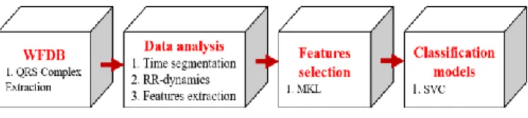
An efficient automated method for AF diagnosis is investigated based on multi-dynamics analysis of QRS time series signal. In such case, we have demonstrated that a dynamical state is better characterized by employing different physical characteristics [13]. For this reason, six different dynamics of the QRS time series were employed to characterize a heartbeat signal, instead of counting on a single RR interval dynamic. As well, 12 linear and nonlinear functions were implemented to convert each RR interval dynamic into 12 features. Hence, a set of 72 features were extracted from the six RR dynamics. The data used in this study is provided from PhysioBank free accessible databases. To clarify, we have combined the three-following databases: AF Termination Challenge Database; Long-Term AF Database; and MIT-BIH Arrhythmia Database. Thereafter, the operation procedures performed in this study were separated into four parts as shown in (Fig.1).

Figure 1: Data processing blocks

The first part is ECG signal reprocessing to extract the QRS complex; the second part is dedicated for data analysis; the third part is feature selection process; and finally, the last part is for the training of the classification models.

Firstly, WFDB (WaveForm DataBase) Software Package-Physionet is used to extract the QRS complex from each ECG recording [14]. WFDB is a set of MATLAB functions and

A Novel Method to Identify Relevant Features for Automatic

Detection of Atrial Fibrillation

(3)

wrappers for reading, writing, and processing files in the PhysioBank databases formats. The WFDB process is used to generate two vectors: the first one concerns R-peaks location in the QRS complex (Fig.2) and the second shows the annotations of each interval. These are executed using the command “rdann” - read a WFDB annotation file.

Figure 2. ECG signal with different waves

1) Data analysis

An algorithm for data analysis is implemented, includes the following operation: (1) time segmentation; (2) RR-dynamics calculation; and (3) features extraction.

a) Time segmentation & RR-dynamics calculation

The R-peaks signal extracted by the WFDB process must be segmented. A time window of 30-second was chosen to divide this R-peaks signal into M short segments Ri_{of 30}

seconds duration, as defined by:



1 2 3 M



peaks

R  R , R , R ,..., R (1) For example, in the ideal case, when the signal is regular, and the heart rate is constant. The R-peaks signal of 3600 seconds (1-hour), will be segmented into 120 segments. For each has a 30-second duration, in the case where the slip pitch equal to 30 seconds.

Generally, the slip pitch must be lower or equal to the splitting window. In the current study, a slip pitch equal to 30-second has been chosen. So, once the R-peaks signals have been segmented, then the six RR dynamics will be computed using the following formulas:

- First dynamic: 1 i i RR R (2N)R (1N 1) (2) - Second dynamic:





2 1 1 RR abs RR (2N)RR (1 N 1) (3) - Third dynamic:



2 2



3 1 abs RR (2 N) RR (1 N 1) RR RR (2 N)       (4) - Fourth dynamic:



2 2



2 N 1 N 1 s 1 2 N s s 4 2 N 1 N 1 1 2 N 1 abs RR (x x ) RR (x x ) RR RR (x x ) RR (x x ) RR (x x ) RR RR (x x )              (5) - Fifth dynamic:









2 2 2 N 1 N 1 s 1 2 N s s 2 N 1 N 1 5 1 2 N 1 abs RR (x x ) RR (x x ) RR RR (x x ) abs RR (x x ) RR (x x ) RR RR (x x )              (6)

- The sixth dynamic:





2 2 s 2 N 1 N 1 1 2 N s s 2 N 1 N 1 6 1 2 N 1 RR (x x ) RR (x x ) RR RR (x x ) abs RR (x x ) RR (x x ) RR RR (x x )              (7)

Where N is the number of components in the RRi_dynamic

used to calculate the next dynamic RRi+1_{. In fact, increasing}

the data-variability by combining different dynamical state of the QRS time series can provide effective characteristics, which serve to constitute a powerful clinical decision support.

b) Features extraction

Various measures of complexity were developed to compare time series and distinguish regularity, chaotic and random behavior. Thus, linear and nonlinear functions have been used to expose RR dynamics as features. For a better understanding, an index “i” was used to differentiate between dynamics, and a parameter N to represent the number of components in the ith_dynamics.

(1) Linear analysis

Mean: Mean value of RR components within each segment. For any vector made up of N scalar observations, the mean is defined as:

 

N i i n 1 1 Mean RR RR (n) N  

_

(8)

RMSSD: is a time-domain method used to quantify the Rate Heart Variability (HRV). This refers to the root mean square of successive RR components within each segment.

We put:

i i

XRR (2N)RR (1N 1) (9) The root-mean-square of a vector X is

 

N ₂ n 1 1 RMSSD X X N  

_

(10)

MMedians: This refers to the median of medians, calculated by dividing the RR interval into three segments. Each segment was centralized by subtracting his own average value. Then, we calculate the median for each segment. And finally, a median of the three medians was calculated.

(4)

SDSD: This refers to the standard deviation of differences between the adjacent RR components within each segment.

 

N 2 n 1 1 STD X X Mean(X) N 1 _   



(11)

Kurtosis: is the ratio of the fourth moment and the second moment squared.

 





 





4 N i i n 1 2 2 N i i n 1 RR (n) Mean RR Kurtosis N RR (n) Mean RR      _     



(12)

Skewness: is the ratio of the third moment and standard deviation cubed.

 





 





3 N i i n 1 3 2 2 N i i n 1 RR (n) Mean RR Skewness N RR (n) Mean RR      _     



(13) (2) Non-Linear analysis

Nonlinear functions were investigated also to characterize the studied arrhythmia. Four functions are based on the scatter plot of the RR segment [3].

VAI: Vector Angular Index is calculated as:



N



n n 1

VAI



_  45 N (14) Where _n is the angle between the line plotted from every scatter point to the original point and the x-axis, N is the number of scatter points.

VLI: Vector length Index is calculated as:



N 2



i n 1

VLI



_ (lL) N (15) Where (l ) is the length between every scatter point and the _i original point, L is the mean of all the (l ), and N is the number _i of scatter points.

SD1: is the standard deviation calculated as:



i i



n 1 n

SD1var RR _ RR 2 (16) SD2: is the standard deviation calculated as:





 



i i i



n 1 n SD2var RR _ RR 2  2 Mean RR (17) Where RRin RR (1i  N 1), i i n 1 RR  RR (2N), and the Var .

 

is the standard deviation.

The five remaining functions were based on different types of entropy which provide a valuable tool for quantifying the regularity of physiological time series. For each type of entropy, a set of certain common parameters is needed to be initialized: embedding dimension m, tolerance threshold r, and time series length N. Following recommendations of some

works dealing with these parameters, m was set at 2 and r represents 20 or 25% of the standard deviation RR segment [15]. In the present study, the following entropy methods have been employed.

ApEn: Approximate entropy was developed by Pincus [16] as a measure of regularity to quantify levels of complexity within time series.

SampEn: like ApEn, Sample entropy is a measure of complexity. But it is different from ApEn mainly by two points: (1) SampEn does not count self-matches; (2) SampEn does not use a template-wise approach [4].

FuzzyEn: Fuzzy entropy, a new measure of time series regularity. Like the two existing related measures ApEn and SampEn, FuzzyEn is the negative natural logarithm of the conditional probability excluding self-matches and considering only the first N-m vectors of length m. There are three parameters that must be fixed for each calculation of FuzzyEn: m, r, and n defined as the gradient of the boundary of the exponential function [17].

COSEn: called coefficient of sample entropy, has a high degree of accuracy in distinguishing AF from NSR in 12-beat calculations performance [5].

QSE: Quadratic entropy rate, based on densities rather than probability estimates. To normalize the value of r, SampEn was modified by dividing the probability by the length of the overall tolerance window 2r [5].

All these 12-linear and nonlinear functions were applied on each dynamic. As results, a set of 72 features was formed. Next, an algorithm based on MKL approach is developed for the feature selection process.

B. MKL Approach to feature selection

This paper suggests the application of MKL approach to solve features selection problem, with special emphasis on heartbeat signal. Indeed, 72-features were extracted from the data, then to improve the learning efficiency of the classifier and the reliability of the model, these features were optimized and reduced to only 13 features by MKL approach.

1) The general framework of MKL algorithm

MKL approach, considered conic combinations of kernel matrices for classification, leading to a convex quadratically constrained quadratic program. Most published studies on MKL are focused on two issues, (i) how to improve the classification accuracy of MKL, and (ii) how to improve the learning efficiency. The reason to use MKL is its ability to learn from a larger predefined set of kernels and parameters an optimal linear (or nonlinear) combination of kernels. Thus, instead of creating a new kernel, MKL algorithm can be used to combine kernels already established. In such case, a convex combination of M basis kernels is computed by





M





i j m m i j m 1 M m m m 1 K x , x w K x , x w.r.t w 0, w 1    _    _ _ 



(18)

(5)

for each training data of couple-subject {i ; j} = 1 ,..., N, where N is the number of subjects p

i

x  presented by p-components (p-features).

All the inputs can be represented as matrix given by:

1 2 p 1 1 1 1 1 2 p 2 2 2 2 1 2 p N N N N x x x x x x x x X x x x x              _{ } _             (19)

Then, each kernel matrix Km applied to X is computed as

follows: m 1 1 m 1 2 m 1 N m 2 1 m 2 2 m 2 N m m N 1 m N 2 m N N K (x , x ) K (x , x ) K (x , x ) K (x , x ) K (x , x ) K (x , x ) K K (x , x ) K (x , x ) K (x , x )       _ _     (20)

The reported SimpleMKL approach solves the kernel problem, through a primal formulation involving a weighted ℓ2-norm regularization, while the ℓ1-norm constraint on the vector w is a sparsity constraint that will force some weights wm to be zero [10]. Further, the solution of the primal MKL

problem is calculated by considering the following optimization formula:

m m

w _m

min F(w), such that



w 1, w 0, m (21) Where:





n M n i j i j m m i j i i, j 1 m 1 i 1 i n i i i 1 1 y y w K x , x max 2 F(w) 0 C subject to : ; i y 0       _ _{ } _{ }          _ _  _     



(22)

To solve (21) a simple gradient method was used. Then, to solve (22) we call an SVM solver. F(w) is considered as an objective function that should be minimized by updating the weights w using a descent direction ensuring that the equality constraint and the non-negativity constraints on w are satisfied. Further, F(w) is expressed by the same problem announced by (Boser et al [18]; Cortes and Vapnik [19]), considering the Lagrangian formulation using the combined kernel.

2) feature selection process

In this study, the MKL approach was developed to perform a feature selection process. So, instead of calculating the combined kernel as used in (18) (or each Gram matrix Km is

computed on a training data set of couple-subject, as shown in (20)), we suggest studying the combined kernel as a convex combination of p-basis kernel given as:





p





m m i j m m i j m 1 K x , x w K x , x ,  



(23)

Or each Gram matrix Km is computed on a training data set

of couple-features, not couple-subject, such as:

m m m m m m m 1 1 m 1 2 m 1 N m m m m m m m 2 1 m 2 2 m 2 N m m m m m m m m N 1 m N 2 m N N K (x , x ) K (x , x ) K (x , x ) K (x , x ) K (x , x ) K (x , x ) K K (x , x ) K (x , x ) K (x , x )                (24)

Where x_im p is a scalar, which means the component m of the subject i {1, …, N}, and m {1, …, p}.

In the original approach, to calculate the combined kernel in (18), the user selects a desired number of kernels. However, in this novel approach, the number of kernels requested is fixed by the number of features (p = 72). Where each Gram Matrix Km is selecting one single feature “m” every-time, {m = 1, …,

p}. Which means that all Gram Matrices Km described in (18)

use the same kernel function, while the selected input feature changes. Therefore, the Eq. 24 is rewritten as:





m m m m m m 1 1 1 2 1 N m m m m m m 2 1 2 2 2 N m m m m m m m N 1 N 2 N N K(x , x ) K(x , x ) K(x , x ) K(x , x ) K(x , x ) K(x , x ) K , m 1,..., p K(x , x ) K(x , x ) K(x , x )       _ _         (25)

Hence, the problem of data representation through the kernel is replaced by the choice of weights wm.

Thus, the problem (22), becomes:



i j



p n n m m i j i j m i i, j 1 m 1 i 1 i n i i i 1 1 y y w K x , x max 2 F(w) 0 C subject to : ; i y 0       _ _{ } _{ }    _     _ _  _     



(26)

So, the process will be started by solving (26). First, all the components wm were initialized by 1/p, then the objective

function F(w) will be computed using an SVM solver.



i j



p n n m m i j i j m i i, j 1 m 1 i 1 1 _{ˆ ˆ} _ˆ F(w) y y w K x , x 2     



 



 



(27)

Where ˆ maximizes (26). After F(w) is calculated, we need to solve (21). So, we compute the derivatives of F(w) as if ˆ does not depend on w.

i j m m i j i j i, j m F 1 _{ˆ ˆ y y K(x , x ),} m w 2  _{ } _{ } _ 



(28)

Then, the reduced gradient of F(w) is computed as:





m u red m m u _m _u F F , for m u w w F F F , for m u w w     _ _  _ _     _ _    __ _ _ _  _ _ _ _  (29)

Where w is the greatest component in w and u its index. _u This gives the descent direction for updating w as:

(6)

m m m u m m m u m u _m _u w 0 F F 0 if w 0, and 0 w w F F D if w 0, and m u w w F F if m u w w       _ _ _ _  _ _      _ _     _ _ _ _  _ _ _ _  _  _ 



(30)

Once the gradient of F(w) and the descent direction D were computed, we start the process of updating w using the formula:

max

w  w D (31) Or _max is the maximal admissible step size headed by D, and calculated by:

max wv Dv    (32) Where:  m  m m m/ D 0 v arg min w / D    (33)

We replace (32) in (33), then we get:

v v

w  w ( w D ) D (34) After the first update, F*_{(w) will be computed using an}

SVM solver with K



_mw K ,ˆ_m _m where ˆw w  _maxD. Then, we check if the objective value decreases or not {F*_(w)

< F(w)}. In the first iteration we set {F*_{(w) = F(w)}. If the}

objective value decrease, w is updated using the formula

max

w  w D. The maximal admissible step size corresponds to a component wv set to zero. This procedure is

repeated until the objective value F*_{(w) stops decreasing. To}

end up the process, an optimal step size  will be calculated by applying the golden search method (one dimensional line search) on the interval between 0 and _max,with an appropriate stopping criterion, such as the Armijo rule, to ensure global convergence. Then the last adjustment is executed to compute the optimal value of w asw  w D.

Finally, all the algorithm procedure is terminated when a stopping criterion is achieved. This stopping criterion can be either based on the duality gap, the KKT constraints, the variation of w between two consecutive steps, or, a maximal number of iterations. In this current study, the MKL duality gap has been chosen.









n i j i j m i j m _{i, j 1} n * i j i j m m i j i, j 1 m

DyalGap DualOne DualTwo

ˆ ˆ DualOne max y y K x , x Where : ˆ ˆ DualTwo y y d K x , x        _ _{ }    _ _{ } 



(35)

Consequently, the process will be terminated when ,

DualGap where  a tolerance threshold.

When the process is over, we look for all weights wm equal

zero, which means that their corresponding Gram Matrix Km

has been eliminated. Thus, all weights wm strictly greater than

zero



w_m0



, represent the location of the features used to constitute the optimal combination of kernels Km.

For an extracted vector w of weights, we select all the indices m corresponding to the nonzero components of wm.

We call by S the subset of the selected features given by:{

mS, if w_m 0}. In this direction, these features will be chosen as the most appropriate combination class to solve the MKL problem.

Subsequently, to evaluate the performance of selected features, a classification algorithm based on SVC is implemented.

III. RESULTS

In this study, two rhythms episodes of AF and NSR were extracted from the three-following databases: AF Termination Challenge Database; Long-Term AF Database; and MIT-BIH Arrhythmia Database. Then, an SVC-based classifier model, with and without MKL, was constructed, either using the whole set of features or a reduced subset. Each SVC model was optimized by using various configurations including the kernel function (Linear function, polynomial function, radial basis function), its corresponding adjustment coefficients, and the regularization parameter C. To get the optimal classification efficiency, setting of the aforementioned parameters must be conducted on a training dataset and validated on the test dataset.

For MKL to feature selection process: Once the selection process is done, we selected features through the weights values of w. Depends on the choice of kernel settings and parameter C, various subsets of features were produced. Each selected subset will be connected to an SVC classifier to evaluate their performance (Fig.3). According to the current framework, we are interested in a subset that combines a minimum number of kernels. Obviously, it comes back to select the combinations that use a minimum number of features. The best result was achieved by combining 13 features.

(7)

In this study, each model was built and validated on a large database combining 70133 NSR and 65698 AF episodes. The performance of the proposed models is detailed in Tab.1 and Tab.2.

Table 1: Recognition rate of NSR and AF using 72 input features.

Model I FA NSR

Learning

Number of segments 2356 2822

Recognition rate for each class 100% 100% The overall recognition rate 100%

Validation

Recognition rate for each class 99.49% 99.65% The overall recognition rate 99.57%

Test

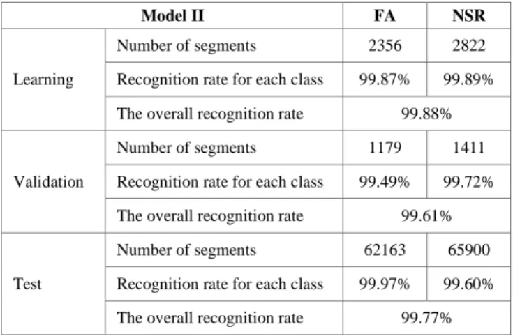
Table 2: Recognition rate of NSR and AF using 13 input features.

Model II FA NSR

Learning

Validation

Test

IV. CONCLUSION

The main purpose of this work is to construct a rapid and efficient diagnostic method able of exploiting short heartbeat segments for an accurate automatic medical monitoring. We targeted six dynamics of heart rate signal, each was segmented into a 30-second window and transferred via 12 linear and nonlinear function to extract a large set of 72 predictors that characterize the most common sustained arrhythmia, AF. Then, an MKL approach was designed to remove non-informative and irrelevant features, so that only 13 features led to the constitution of a more accurate classifier. As well, we aimed to demonstrate for the first time that MKL could be successfully applied to feature selection task for machine learning pipelines. The reported performance achieved 99.77% for an SVC model use MKL feature selection process, and 99.68% for an SVC model without MKL. Firstly, these results clearly show that the idea of using an MKL approach to perform feature selection tasks is succeeded. Secondly, we managed to detect the AF episodes with a very important

recognition rate of 99.97% on a database contains 62163 segments, applying 13 features.

REFERENCES

[1] S. Levy, G. Breithardt, RW. Campbell, AJ. Camm, JC. Daubert, M. Allessie, et al. Atrial fibrillation: current knowledge and recommendations for management. Working Group of Arrhythmias of the European Society of Cardiology, European Heart Journal, 19, (1998), 1294-320.

[2] Z. Haddi, JF. Pons, S. Delliaux, B. Ananou, JC. Deharo, A. Charaï, R. Bouchakour, M. Ouladsine. A Robust Detection Method of Short Atrial Fibrillation Episodes, Computing in Cardiology,44, (2017), 1-4.

[3] R. Xiuhua, L. Changchun, L. Chengyu, W. Xinpei, L. Peng, Automatic detection of atrial fibrillation using R-R interval signal, BMEI, 2, (2011), 644 – 647.

[4] JS. Richman, JR. Moorman, Physiological time-series analysis using approximate entropy and sample entropy, American Journal of Physiology, Heart and Circulatory Physiology, 278, (2000), 2039.

[5] DE. Lake, JR. Moorman, Accurate estimation of entropy in very short physiological time series: the problem of atrial fibrillation detection in implanted ventricular devices, Am J Physiol Heart Circ Physiol, 300 (2011), 319-25.

[6] Z. M. Hira, D. F. Gillies, A Review of Feature Selection and Feature Extraction Methods Applied on Microarray Data, Adv Bioinformatics. (2015), 198363.

[7] G. Lanckriet, N. Cristianini, P. Bartlett, and L.E. Ghaoui, Learning the kernel matrix with semi-definite programming, J. Mach. Learn. Res, 5, (2004), 27–72.

[8] S. Sonnenburg, G. Rätsch, and C. Schäfer, A general and efficient multiple kernel learning algorithm. NIPS, (2006), 1273–1280.

[9] M. Kloft, U. Brefeld, S. Sonnenburg, and A. Zien, lp-Norm multiple kernel learning, J. Mach. Learn. Res, 12, (2011), 953–997.

[10] Z. Xu, R. Jin, S. Zhu, M. Lyu, and I. King, Smooth optimization for effective multiple kernel learning, in Proc. AAAI Artif. Intell., 2010.

[11] M. Kowalski, M. Szafranski, and L. Ralaivola, Multiple indefinite kernel learning with mixed norm regularization, in Proc. 26th ICML, Montreal, QC, Canada, (2009), 545–552.

[12] A. Rakotomamonjy, F. Bach, S. Canu, Y. Grandvalet, SimpleMKL, Journal of Machine Learning Research, Journal of Machine Learning Research, 9, (2008), 2491.

[13] J.F. Pons, Z.Haddi, J.C. Deharo, A. Charaï, R. Bouchakour, M. Ouladsine & S. Delliaux. Heart rhythm characterization through induced physiological variables. Scientific Reports, 7, (2017), 5059.

[14] https://physionet.org/physiotools/wfdb.shtml

[15] S. Lu, X. Chen, JK. Kanters, IC. Solomon, KH. Chon. Automatic selection of the threshold value R for approximate entropy. IEEE Trans Biomed Eng, 55, (2008), 1966-72.

[16] S.M. Pincus, Approximate Entropy as a Measure of System Complexity, Proc. Natl Academy Sci. USA, 88, (1991), 2297–2301.

[17] C. Weiting, W. Zhizhong, X. Hongbo, Y. Wangxin. Characterization of Surface EMG Signal Based on Fuzzy Entropy. IEEE Transactions on Neural Systems and Rehabilitation Engineering, 15, (2007).

[18] C. Cortes, V. Vapnik, Support Vector Networks, Machine Learning, 20, (1995), 273-297.

[19] Boser. B, Guyon. I, Vapnik. V, A training algorithm for optimal margin classifiers, Proceedings of the fifth annual workshop on Computational learning theory – COLT '92, 144.