HAL Id: hal-02354537
https://hal.archives-ouvertes.fr/hal-02354537
Submitted on 7 Nov 2019
HAL is a multi-disciplinary open access
archive for the deposit and dissemination of
sci-entific research documents, whether they are
pub-lished or not. The documents may come from
teaching and research institutions in France or
abroad, or from public or private research centers.
L’archive ouverte pluridisciplinaire HAL, est
destinée au dépôt et à la diffusion de documents
scientifiques de niveau recherche, publiés ou non,
émanant des établissements d’enseignement et de
recherche français ou étrangers, des laboratoires
publics ou privés.
Data Summaries and Representations: definitions and
practical use
Alain Barrat, Ciro Cattuto
To cite this version:
Alain Barrat, Ciro Cattuto.
Data Summaries and Representations:
definitions and
practi-cal use.
Multiplex and Multilevel Networks, Oxford University Press, 2018, 9780198809456.
Data Summaries and Representations:
definitions and practical use
Alain Barrat and Ciro Cattuto
1.1 Introduction
Complex networked data have become available in a variety of contexts, describing a variety of systems with growing abundance of details, such as, for instance, the multiple nature of links between individuals in social networks, or the temporal evo-lution of these links. The availability of such rich datasets describing for instance behavior and interactions of individuals or socio-economic entities is bringing forth both new opportunities and challenges. Data come from heterogeneous sources, at different scales and resolutions, with variable amounts of details or metadata and sometimes temporal resolution. Data alone however, even in huge quantities, do not easily transform into knowledge or predictive models. The richness, level of detail and diversity of data sets raise crucial challenges concerning data analysis, repre-sentation and interpretation, the extraction of structures from data and the practical use of data, be it to compare different systems, explore their temporal evolution, or for the integration of data into data-driven models of interest in contexts such as epidemiology or computational social sciences.
Data need thus to be summarized and represented in simpler forms. To this aim, one needs to understand which characteristics of any dataset under investigation are crucial to retain, which ones on the other hand are too specific to be of gen-eral interest. A data representation will encapsulate the relevant information, while discarding the unnecessary details. Data representations can be more or less sum-marized or coarse-grained with respect to the original data. For any dataset, one can define a number of representations retaining different amounts of information on
Alain Barrat
Aix Marseille Univ, Universit´e de Toulon, CNRS, CPT, Marseille, France and Data Science Labo-ratory, ISI Foundation, Torino, Italy, e-mail: [email protected]
Ciro Cattuto
Data Science Laboratory, ISI Foundation, Torino, Italy, e-mail: [email protected]
the characteristics of the data, and the choice of the most useful representation will depend on the specific goal and on its specific use.
In this chapter, we consider for definiteness the concrete case of temporal net-works. We recall several commonly used data summaries and levels of represen-tation of temporal networks as well as novel data represenrepresen-tations that have been developed through the Multiplex project. We focus in particular on the case of tem-poral networks of contacts between individuals and show in a series of concrete use cases how different representations can be used to characterize and compare data, or to feed data-driven models of epidemic spreading processes.
1.2 Data and representations of data
1.2.1 Datasets, common summaries and representations
Let us consider a dataset describing a temporal network, i.e., a set of nodes rep-resenting for instance individuals, and of links that appear and disappear between these nodes. This is the case of the numerous datasets of face-to-face contacts be-tween individuals collected by the SocioPatterns collaborations or by other groups in a number of countries and contexts including schools, hospitals, scientific confer-ences, museums, etc. Each such dataset is typically of the following detailed nature: For each pair of individuals i and j, the dataset contains a list of ` “events”, i.e., successive time intervals ((ti j(s,1),ti j(e,1)), (ti j(s,2),ti j(e,2)), · · · , (ti j(s,`),ti j(e,`))) during which iand j were detected to be in close-range face-to-face proximity, where ti j(s,a)refers to the starting time and ti j(e,a)to the ending time of the time interval number a. Note that in a number of temporal networks, such as networks of communications be-tween individuals, the durations of the events are neglected, so that each event is composed only of one timestamp. While this representation contains all the avail-able data, and hence retains all the availavail-able information, it entails some disadvan-tages. On the one hand, the visualization of time-evolving networks is challenging, making it difficult to grasp its structures and features. On the other hand, a spe-cific dataset is often unique, and differs from other similar datasets describing for instance the same system at another time, or similar systems. Examining the full dataset without using the lens of coarse-grained representations or summaries can then inhibit the search for commonalities and robust patterns or properties. For in-stance, the detailed face-to-face contacts that occur in a specific school on a specific day are certainly unique, but bear some important similarities with the contacts of another day in the same school, even if they do not repeat in the same way every day. Using summaries and representations makes it possible to highlight similarities and pinpoint important differences between similar datasets.
Statistics.
The first type of data representation that is customarily used consists in building statistics for several quantities of interest. For instance, the temporal evolution of the number of events per unit time can inform us on circadian patterns in the data, on the possible recurrence of moments of high and low activity. The evolution of the number of events involving each individual, as well as of the number of distinct other individuals with whom an event is shared, can also reveal interesting patterns. Moreover, the list of contact time intervals yields for each pair of individuals i and j a list of contact durations (∆ti j(1), · · · , ∆ti j(`)), with ∆ti j(a)= ti j(e,a)− ti j(s,a) for a= 1, · · · , `. The distributions of these contact durations, as well as of the time intervals between contact events, have been found to be broad in many datasets: most contact durations and intervals between successive contacts are very short, but very long durations are also observed, and no characteristic timescale emerges. This bursty behavior is a well known feature of human dynamics and has been observed in a variety of systems driven by human actions, with important consequences on processes unfolding on temporal networks.
While these properties are of course of interest, they certainly do not reveal enough to fully characterize a dataset. Strikingly, a number of temporal network characteristics are in fact defined through the use of another more coarse-grained representation, which is widely used and sometimes implicitly considered: the tem-porally aggregated networks.
Aggregated networks.
The sequence of events between the nodes of a temporal network during a given time window defines an aggregated network, which is a static summary of the temporal network. Taking once again the example of temporal contact networks, each node of the aggregated network is an individual, and a link between two nodes i and j denotes the fact that the corresponding individuals have been in contact at least once during the time window under consideration. The bare structure of this graph encodes information on the overall topological structure of the temporal network, but not on its temporal properties. In order to retain some temporal information, it is customary to summarize the temporal activity of individual edges i- j by suitably defined weights for the edges. Several notions of weight wi j for the edge i- j can
be defined on the basis of the list of contact durations, yielding weighted contact networks that describe different aspects of the empirical sequence of contacts: • edge presence: wi jp measures the contact occurrence (the superscript p stands
for “presence”), with wi jp = 1 if at least one contact between i and j has been established, and 0 otherwise;
• frequency of occurrence: the frequency wn
i j= l indicates how many distinct
con-tact events have been registered between i and j, disregarding the length of each contact (the superscript n is for “number”);
• cumulative time in contact: the cumulative duration of the contact wt
i j= ∑a∆ t (a) i j
gives the sum of the durations of all contacts established between i and j. The time window considered for aggregation can range from the finest time res-olution of the data up to the entire duration of the data set. In many contexts, it is natural to consider a specific temporal aggregation scale (i.e., daily), but different aggregation levels typically provide complementary views of the network dynamics at different scales.
The aggregated network representation carries both advantages and limitations. An important interest of aggregated networks lies in their static nature: this makes them amenable to the usual characterization tools of network analysis and visual-ization: degree distributions, clustering, assortativity, etc. The comparison of their structures across contexts can unveil important information about the contact pat-terns of the population, as we will see later on concrete examples. Moreover, the assignment of weights to links allows to keep track of important characteristics such as the heterogeneity of the number and durations of contact events between differ-ent pairs of individuals, and of higher order correlations between the numbers and durations of events between individuals.
The aggregation on successive time windows sheds also light on the temporal evolution and possible stability of the system under scrutiny. This can be done at different levels of detail, from a comparison of (degree, weight, strength) distribu-tions measured on different time windows, or a measure of a similarity such as Jac-card coefficient between successive aggregated networks. Such measure can even be used to automatically detect relevant timescales in temporal networks [1]. At a finer resolution, we can investigate the similarly between the neighborhoods of a given node in contact networks aggregated over different periods. For instance, for daily aggregated networks, the similarity between the neighborhoods of an individ-ual i in the contact networks measured in two different days denoted 1 and 2 can be quantified through the cosine similarity σ1,2(i) = ∑
jwi j,1wi j,2/
q
∑jw2i j,1∑jw2i j,2,
where wi j,dis the weight of the link between i and j in the contact network of day d,
i.e., the cumulative duration of the contacts between i and j occurring on day d. The cosine similarity takes values between 0 and 1: it is equal to 0 if i had contact with strictly different individuals in the two days considered, and to 1 if i had contacts with the same persons in both days, with proportional durations.
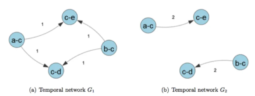
Obviously, aggregated networks have also limitations. The main one stems from the fact that they do not carry information on the order of events. Different temporal networks with different histories can thus give rise to the same aggregated weighted network, as shown for an example in Fig. 1.1. This can turn out to be crucial when dealing with processes on temporal networks: if for instance A and B come into con-tact before B and C do, A can transmit an information to C through B while, if the order of contacts is reversed, this propagation path does not exist. A static represen-tation does not distinguish between these possibilities and therefore overestimates the existence of paths between nodes. As a result, aggregated networks can yield misleading results on the relative importance of nodes in the network (as measured, e.g., by their centralities) [2, 3, 4].
Fig. 1.1 Time-unfolded and weighted static, time-aggregated representation of two temporal net-works G1and G2: two different temporal networks can yield the same aggregated weighted
net-work. From [4].
Contact matrices.
When the population described by the data at hand can be divided into groups, such as for instance age groups, or classes in a school context, departments in offices, etc, it is customary to describe the contact networks between specific groups of individuals by using contact matrices, which contain very coarse summaries of the data but highlight the mixing patterns between these groups. If the population is divided into n groups, and if we denote the number of individuals in group X by nX,
one usually considers the following quantities, aggregated over each time window of interest:
• the total number of contacts between individuals of class X with individuals of group Y : NXY = ∑i∈X, j∈Ywni j(for X = Y we have NX X=12∑i, j∈Xwni j),
• the average number of contacts of an individual of group X with individuals of group Y nXY = NXY/nX,
• the total time spent in contact between individuals of group X with individuals of group Y : WXY = ∑i∈X, j∈Ywti j(for X = Y we have WX X=12∑i, j∈Xwti j),
• the average time spent by an individual of group X in contact with individuals of group Y : wXY = WXY/nX.
Contact matrices contain thus an even more coarse-grained representation of the data than aggregated networks: the differences between individuals of a group are neglected, as is the specific structure of the contact network, since only averages are retained. They are however widely used to inform data-driven models of spreading processes in the epidemiology of infectious diseases: when dealing with diseases that affect in different ways persons of different ages for instance, it can indeed be crucial to take into account the fact that children have more contacts among them than adults, with therefore a higher propagation risk. The specific structure of the contact networks of children and adults might on the other hand be less relevant. In
this respect, the simplicity of contact matrix representations is appealing. Moreover, even such a simple representation can carry interesting information on the temporal stability of the mixing patterns between groups: one can for instance consider the similarity between two contact matrices measured in different time windows, which can inform us on the differences between the mixing patterns of children and adults during schooldays vs weekends or vacations.
1.2.2 Novel data representations
The above description of the data representations highlights the need for novel in-termediate ways of representing temporal networks. On the one hand, keeping too much detail can limit the ability to generalize data. On the other hand, aggregated temporal networks, even if weighted, do not take into account enough temporal information to correctly rank nodes by their importance and overestimate the exis-tence of paths between nodes; contact matrices in addition do not take into account the heterogeneity of links and nodes within a group and discard any structure, and in particular the fact that not all pairs of nodes are linked.
Within the Multiplex project, two complementary directions have been followed, developing novel frameworks for the representation of temporal network data. Im-portantly, both correspond to static representations, hence much easier to deal with than temporal ones, but retain more temporal information than the representations discussed above.
Higher order aggregated networks.
A first important issue, given a temporally resolved dataset, consists in determin-ing in which measure an aggregated representation gives inaccurate information on the real data. To this aim, the betweenness preference has been introduced in [3]: it quantifies to which extent paths existing in time-aggregated representations of temporal networks are actually realizable in the time-resolved data. In other words, measuring betweenness preference in empirical temporal networks allows to under-stand if the corresponding aggregated representations loose too much information or can be used for the simulation of dynamical processes unfolding on these networks. As discussed above, static representations of temporal data are however of great interest. To go forward in this perspective, several authors have therefore introduced new higher-order time-aggregated representations of temporal networks [5, 6] that take into account non-Markovian effects and thus preserve causality. An example is given in Fig. 1.2 for second-order aggregation: each second-order node represents an edge in the first-order aggregate network G(1); second-order edges are given by all pairs (e1, e2) of directed edges of type e1= (a, b) and e2= (b, c) in G(1), i.e.,
by all possible paths of length two in the first-order aggregate network. Second-order edges are moreover weighted, and the weights w(2)(e1, e2) can be defined as
the relative frequency of time-respecting paths (a, b;t1) → (b, c;t2) with t2> t1of
length two in the temporal network.
Representing data in this way, instead of simply aggregating temporally, allows to keep more information on relevant temporal correlations. For instance, using ran-dom walks on such novel representation preserves the statistics of temporal paths of length 2, i.e., of correlations that can be crucial when simulating dynamical pro-cesses on top of temporal networks, and to create a novel, causality-preserving, null model of temporal networks. This representation has allowed to show for in-stance that non-Markovian characteristics of temporal networks can either enforce or mitigate the influence of topological properties on dynamical processes. As such, they constitute an important additional dimension of complexity that needs to be taken into account when studying time-varying network topologies [6]. Moreover, the path-based centralities defined in such higher-order aggregate networks give a much better evaluation of the ranking of nodes’ importance in the temporal network than when the usual aggregated networks are used [4].
Fig. 1.2 Second-order aggregate networks corresponding to the two temporal networks shown in Fig. 1.1. From [4]
Contact matrices of distributions.
The contact matrices of distributions (CMD) extend the usual concept of contact matrices to tackle their shortcomings while maintaining a highl level of summariza-tion of complex temporal data. In practice, the matrix defined in [7] has as entry for groups X and Y the distribution of aggregated contact durations between all pairs of individuals x in group X and y in group Y, where the distribution includes the fraction of such pairs that do not have any contact. Alternatively, it is possible to fit all the distributions to a common functional form (in [7], a negative binomial distribution) and to consider as entries of the matrix the parameters of the fits. Sim-ilarly to the customary contact matrices, the contact matrix of distributions is not an individual-based representation: it does not retain the detailed structure of the empirical contact network and contains only a summary of all interactions between
individuals of various groups. However, in contrast with the usual contact matrices, it accounts for the broad fluctuations of contact durations as well as for the poten-tially high fraction of missing links across groups of individuals (it does not assume that all individuals have been in contact).
It is important to note that the CMD defines in fact a representation framework that can be extended and refined in various ways. For instance, while the CMD of [7] contains only the distribution of daily aggregated contact durations, one can retain as entry of the matrix the more detailed distributions of (i) durations of single contacts (ii) intercontact durations and (iii) number of contacts between pairs of individuals, as well as the density of links between groups. Keeping this information allows one to build realistic timelines of contacts between individuals that respect these statistics, as we will see in the next section [8]. Moreover, matrix entries could also retain clustering coefficients of the aggregated networks, or their assortativity properties, or other temporal or structural properties considered relevant.
1.2.3 Detecting mesoscopic structures
The representations discussed above are based on aggregation over time or over node attributes, projecting away many specificities, structures, and correlations of the original data. Depending on the problem at hand, these aggregated representa-tions may overlook or confound important structural features of the network. For example, a node may belong to different communities at different points in time: aggregating the network over time will artificially merge the communities and cre-ate a cluster that does not represent the network at any point in time. Groups of nodes with similar activity patterns over time can also exist: for instance in environ-ments such as schools, the interactions that are possible at a given time are driven and constrained by an externally imposed schedule of social activities (e.g., class and lunch breaks). In this case, temporal aggregation of the network may retain the topology of interactions but loses the information on correlated activity patterns, which may play an important role for, e.g., epidemic processes unfolding over the temporal network [9]. In general, correlated topological and temporal features of the network may give rise to structures that are neither local features of individual nodes or edges nor global structures, and are hence often called ”mesostructures”. Detecting such mesoscopic structures in high-resolution social network data is an out-standing challenge that goes beyond the extension of community detection tech-niques to temporal networks.
In this perspective, a promising approach uses a tensor representation of the tem-poral network: one start by representing the temtem-poral network as a time-ordered se-quence of adjacency matrices, each describing the state of the network at a discrete point in time. The adjacency matrices are then combined into a three-way tensor that encodes the entire information about the temporal network and has been recognized as a convenient representation both for multi-layer networks and temporal networks. As shown in [10], non-negative tensor factorization techniques, which have shown
their relevance in the field of machine learning, can then be used to extract non-trivial structures and represent such complex data as a sum of simpler terms that can be more easily interpreted. Interestingly, some of these structures correspond to so-called ”communities” in static networks, but others entail a complex inter-play of activity and structural patterns that could not be found by usual community detection tools. This opens the door to representing information-rich complex data in simpler, human-readable ways and also to investigations on how each simpler structure impacts dynamical processes unfolding on these data, as we will discuss below.
1.3 Putting the data representations to concrete use
1.3.1 Comparing datasets
In the task of comparing datasets, to assess for instance the robustness of stylized facts concerning the system(s) of interest observed at different moments or under different conditions, even very simple and coarse-grained representations are ex-tremely valuable. For instance, statistical distributions of contact durations and their functional shapes can be compared in datasets describing contacts between individ-uals collected in different contexts [11, 12, 13, 14, 15, 16]: as shown in Fig. 1.3, the distributions of contact durations are very broad, and extremely similar for very different contexts, populations, activity timelines, and deployment conditions. The broadness of these distributions, as well as their robustness, imply two important facts for modelers, in particular when dealing with processes depending on contact durations between individuals, such as epidemic spreading. First, the broadness of the distributions means that taking into account only average contact durations and assuming that all contacts are equivalent might be a too coarse representation of the reality. Indeed, different contacts might yield very different transmission probabil-ities: many contacts are very short and correspond to a small transmission proba-bility, but some are much longer than others and could therefore play a crucial role in disease dynamics, Second, the robustness of the distributions found in different contexts means that these distributions can be assumed to depend negligibly on the specifics of the situation being modeled and thus directly plugged into the models.
Longitudinal studies can also be carried out at the level of coarse-grained sum-maries. For instance, the distributions of contact or inter-contact durations have been shown to be robust also when measured in different time windows, unveiling a sta-tistical stationarity in an otherwise non-stationary signal. Activity timelines giving, e.g., the number of contacts between individuals of different groups, can turn out to be very stable from one day to the next, as for instance in hospitals or schools [16, 13, 15], or to have a more casual character as in offices [14], giving hints on the impact of organizational details on contacts. Contact matrices giving the average number or duration of contacts between individuals of different categories have also
Fig. 1.3 Distributions of the face-to-face contact dura-tions measured in different environments ranging from a museum (SG) to a school (PS) and several scientific conferences. 101 102 103 104 ∆tij 10-6 10-5 10-4 10-3 10-2 10-1 100 P( ∆ t ij ) SG HT09 SFHH ESWC09 ESWC10 PS
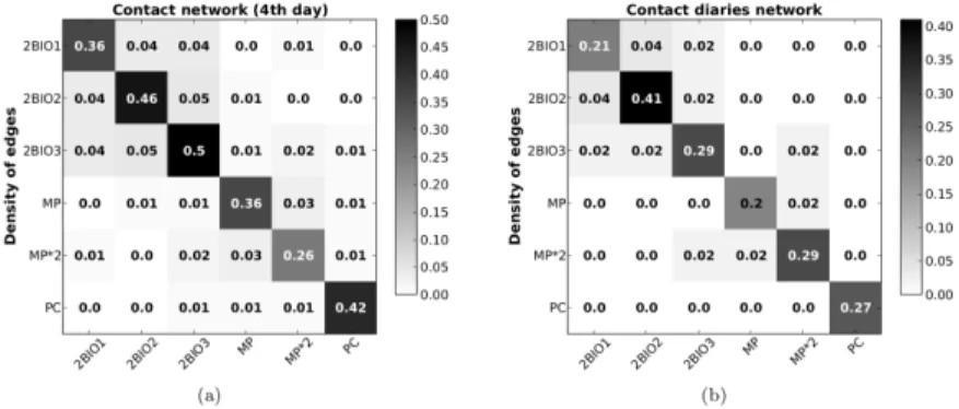
revealed an interesting robustness of contact patterns in a high school across differ-ent timescales: these contact matrices, computed for the same classes in differdiffer-ent days or even in different years, are extremely similar [13, 15], showing for instance that temporally limited datasets can already yield important information on mixing patterns of students that remain relevant on long timescales. Finally, contact matri-ces built from data coming from different sourmatri-ces, namely on the one hand wearable sensors and on the other hand contact diaries, have also revealed a strong similarity, despite the raw datasets differ qualitatively and quantitatively [15], as shown in Fig 1.4.
Notably, the robustness of both distributions of contact durations and of contact matrices imply the robustness of contact matrices of distributions, a fact that we will exploit below.
Fig. 1.4 Contact matrices of link densities obtained from different data sources in a high school. We compare here the contact matrices of link densities between classes built from (a) the network of contacts obtained using the sensor data collected on a specific day and (b) the network of contacts as reported in the contact diaries collected on the same day. The similarity between these two matrices is of 97%. From [15].
The study of aggregated networks obviously shed more light on the comparison of datasets, by providing additional statistical characteristics such as the distribution of the number of neighbors, of the cumulative contact durations, the correlations be-tween nodes’ properties such as degree and strength, but also by allowing a compar-ison of networks’ structures at both global and local levels. The aggregated contact networks first provide additional properties whose distributions can be measured and compared, such as nodes’ degrees and strengths and links weights. The distri-butions of degree (number of distinct individuals with whom a given individual has been in contact) turn out to be similar across days and contexts, with narrow shapes, an exponential decay at large degrees and characteristic average values that depend on the particular context [2]. The distributions of the cumulative contact durations are broad and very similar across very different contexts: different populations, in which individuals behave with very different goals in different spatial and social en-vironments, display a strikingly similar statistical behavior. Finally, the comparison of the neighborhoods of specific nodes in different days yield information on the rate of renewal of contacts between different days, an important quantity in the context of epidemic spreading phenomena. This rate turns out to be substantial, but much smaller than if contacts were at random, and takes similar values across contexts.
Despite these statistical similarities, aggregated networks describing contacts in different contexts are obviously different, as revealed by a more detailed investiga-tion. Differences in their structure can be already revealed by a visual inspection of simple force-based network layouts. For instance, the aggregated network of in-teractions during a conference day is much more “compact” than the ones describ-ing the interactions between museum visitors. The aggregated network of contacts among school children, high school students or office workers have a more modular structure [14, 15]. For instance, children of each class form a cohesive structure with many links, but links between different classes, and in particular between children of different grades, are less frequent.
More subtle differences can be found by investigating the correlations between weights and network topology. In particular, we can consider for each node its de-gree (number of distinct individuals contacted) and its strength (cumulated time of interaction with other individuals). Correlations between these quantities are ex-pected. For random durations of contacts a linear dependency of the average strength hs(k)i of nodes of degree k is obtained; a super-linear dependence hints at the im-portance of super-spreader nodes with large degree, while a sub-linear behavior in-dicates that the decrease in the weights of individual contacts mitigates the expected super-spreading behavior of large degree nodes. In this respect, contrasting results have been obtained in different contexts, showing that too coarse data summaries ignoring correlations might not carry enough information to fully characterize how diffusion processes would unfold on the contacts described by these data. Aggre-gated networks, even though they do not include detailed temporal information and remain a static description, shed in this respect important light on the system’s dy-namics.
1.3.2 Using detailed data in data-driven simulations
One of the most important practical uses of data consists in feeding data-driven models of dynamical processes such as for instance information diffusion or epi-demic spread, which unfold on networks of communication or contacts. The issue of how much detail should be used when feeding such models is tightly linked with the above discussion on advantages and limitations of data representations.
The answer depends in particular on the timescales of the process under inves-tigation. For instance, when dealing with fast processes, the order in which events between nodes take place can be crucial in determining how fast the process spreads and how many nodes it impacts [9, 6]. On the other hand, for relatively slow pro-cesses such as simulations of realistic infectious disease spread, it has been shown in [11] that aggregated networks can be used as a substitute of full temporal net-work data, under the condition that the aggregated netnet-work is weighted, i.e., that the heterogeneous character of the interaction between individuals is taken into ac-count. In the same spirit, [7] shows how the use of usual contact matrices in data-driven simulations of spreading processes can yield misleading results, while the contact matrices of distributions, which entail a summary of the heterogeneity of contact patterns, come thus as an interesting trade-off to inform models of realistic infectious disease spread, by keeping the right amount of information and forgetting about unimportant details when one is not interested in who is specifically reached by the spread, but rather in population level outcomes and in strategies based on grouping individuals according to their role or category in the population.
We discuss below two more practical uses of contact matrices of distributions and of contact matrices in data-driven simulations.
Using data representations to complement incomplete data
As discussed above, comparison of various datasets describing contacts between individuals has revealed the strong robustness of the distributions of contact dura-tions across contexts. Moreover, these distribudura-tions have been shown to be robust as well under sampling of the population under scrutiny. Contact matrices giving the density of links between groups of individuals are also unchanged by sampling. As discussed and shown in practice in [8], this can be a great resource when dealing with incomplete datasets.
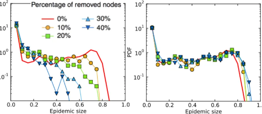
Let us for instance assume that data describing the contacts between individuals has been collected in a given context, but that not all individuals have participated to the data collection. As a result, all information on the contacts involving the non-participating individuals seems to be lost. When simulating a spreading process on the data, these individuals effectively act as if they were immunized as the potential transmission paths going through them cannot be taken into account. The outcome of the spread is therefore strongly estimated [8] (see Fig. 1.5).
The robustness of the CMD under population sampling means however that not all the relevant information about the non-participating individuals is unknown, and
that this data representation can be accurately measured even in the incomplete data. The CMD can then be used to create surrogate data, i.e., sets of fake but realistic timelines of contacts among the non-participating individuals and between them and the participating ones. Using such surrogate data in the spreading simulations allows to recover a correct evaluation of the epidemic risk [8], as shown on an example in Fig. 1.5. 0.0 0.2 0.4 0.6 0.8 1.0 Epidemic size 10-1 100 101 102 PDF
Fig. 1.5 Distribution of epidemic sizes for a spreading process simulated on top of a temporal contact network, here a high school dataset. The red curve gives the distirbution when the whole dataset is used. Left: distributions obtained when data is missing. Right: distributions obtained when surrogate data built using knowledge on the contact matrix of distributions measured on the sampled data are used. From [8].
Another example of the usefulness of such representations has been given in [17]. Contact data obtained through contact diaries, due both to population sampling and to underreporting of contacts, is very incomplete and cannot be used easily in de-tailed simulations of spreading processes. However, the similarities of the contact matrices of link densities measured in both contact diaries and sensor data, together with the wide robustness of the distributions of contact durations measured in verse settings, means that it is also possible to build, starting from the contact di-aries, surrogate contact data that is similar enough to the real contacts so that the outcome of the simulations of spread yields similar results [17]: once again, one uses the robustness of the CMD properties across data sources and contexts to mea-sure the properties of the contacts most relevant for the issue at hand.
These two examples crucially confirm the interest of the contact matrix of dis-tributions, by showing that the information it contains about the density of links between groups of individuals and the heterogenity of contact durations is sufficient in the perspective of using data in simulations of realistic spreading processes.
Mesoscale interventions
Detailed, time-resolved networked data can yield a precise ranking of nodes accord-ing to their importance as measured for instance from their (temporal) betweenness centrality. A customary perspective consists in using such ranking to identify the nodes on which it is interesting to act in order to mitigate or enhance a dynami-cal process such as an epidemic propagation. The ensuing individual-based control strategies, however, are difficult to carry out in practice. Moreover, in the case of temporally evolving networks, they might be of limited efficiency as the specific interactions among nodes do not repeat themselves in a precise way at different moments [18]. On the other side of the possible spectrum of data representations, too coarse summaries of the data, such as global averages, offer only a very limited choice of control tools.
In this perspective, representations of the data at intermediate levels of detail can in fact carry crucial information suggesting efficient interventions at this interme-diate scale. For instance, the contact matrix representation of the contact patterns occurring in a school shows that children spend much more time in contact with children of the same class and of their own grade. This is expected to be a rather general qualitative feature of schools, due both to age homophily and schedule con-straints, and suggests that transmission events might take place preferentially within the same class or grade. Hence, such data suggests targeted and reactive miti- gation strategies in which one class or one grade is temporarily closed whenever symp-tomatic individuals are detected. As shown in [19], these strategies turn out to be almost as effective as whole-school closure, at a much lower cost in terms of service disruption.
Another example of mesoscale intervention is developed in [20] in the context of the decomposition of a temporal network of contacts in a sum of interpretable components thanks to the non-negative tensor factorization [10] described above. Simulations of epidemic spreading processes with varying parameters can indeed be carried out either on the original temporal contact network or on a modified net-work in which a specific component s has been removed (obtained by summing the other components), and the outcomes can be compared. When a component can be interpreted in terms of a specific behavioral pattern, its removal can be regarded as the effect of an intervention strategy that selectively targets that behavior. The case study presented in [20] corresponds to the interactions between children in a school. Its tensor decomposition yields on the one hand components corresponding to the classes, and on the other hand components mixing different classes and correspond-ing mainly to the lunch breaks. As shown in Fig. 1.6, the removal of the latter has a much stronger impact than the removal of the former, despite corresponding to a smaller number of links. Most importantly, such components could not be iden-tified by traditional community detection methods but instead consist of weaker, temporally-localized mixing patterns corresponding to scheduled social activities.
Fig. 1.6 Impact of the removal of specific structures of a temporal network (school dataset) on a SIR spreading process. The heatmap shows the epidemic size ratio (ratio of epidemic sizes without and with intervention) as a function of the spreading model parameters. Each heat map corresponds to a targeted intervention that selectively removes one component. For each removed component r the heat map shows the epidemic size ratio as a function of the SIR parameters λ and µ. Epidemic ratio = 1 indicates that the intervention does not affect epidemic size. The white area is the region where the epidemic dies out, i.e., it fails to affect more than 1% of the network nodes. The region inside the black contour line corresponds to parameter values such that the SIR epidemic finishes within the finite span of the school dataset (2 days), both for the full and the altered temporal networks. That is, for those parameter values the epidemic size ratio is not affected by the finite temporal span of the dataset. The figure clearly shows the strong impact of removing components 12 or 14, which correspond to the mixing of classes during the breaks. From [20].
1.4 Conclusions and perspectives
The increase in data availability and resolution raise both opportunities and chal-lenges related to their analysis, modeling and practical use. Many datasets in par-ticular are commonly used to feed data-driven models. To this aim, the right level of description need to be found, which keeps relevant salient properties of the data while discarding unnecessary details. Adequate data representations and null mod-els need therefore to be defined. Naturally, different datasets can give rise to the same representation, once aggregated. It is thus in fact interesting to define whole hierarchies of representations at intermediate aggregation levels. In this chapter, we have reviewed some recent advances in the case of temporal networks, and dis-cussed their possible representations, from very detailed to very coarse. Each rep-resentation retains specific features of the data. For instance, higher order temporal networks take into account non-Markovian aspects and preserve causality. Contact matrices of distributions keep information about the heterogeneities of contact du-rations between different groups. Mesoscale structures reveal complex interplays of activity and structural patterns. These representations can be used to compare datasets, which can for instance be similar at a certain level of aggregation but dif-fer at a less aggregated one. They can also be useful to feed data-driven models of
dynamical processes or to generate synthetic datasets similar to a given, original one.
Many perspectives and issues remain obviously open. In particular, principled approaches to the design of hierarchies of data representations and null models are currently missing. Further techniques to detect structures and correlated activity pat-terns are needed. It is also important to devise minimal models at different levels of description that incorporate non-trivial longitudinal structures, mesoscopic struc-tures, and correlated activity patterns. Finally, the issue of building approaches to dynamical processes on (temporal) networks by working directly at mesoscales re-mains an outstanding problem.
References
1. Darst, R. K. et al. Detection of timescales in evolving complex systems. ArXiv e-prints (2016). 1604.00758.
2. Isella, L. et al. What’s in a crowd? Analysis of face-to-face behavioral networks. Journal of Theoretical Biology271, 166–180 (2011).
3. Pfitzner, R., Scholtes, I., Garas, A., Tessone, C. J. & Schweitzer, F. Betweenness preference: Quantifying correlations in the topological dynamics of temporal networks. Physical Review Letters110, 198701 (2013). URL http://link.aps.org/doi/10.1103/PhysRevLett.110.198701. 4. Scholtes, I., Wider, N. & Garas, A. Higher-order aggregate networks in the analysis of
tem-poral networks: path structures and centralities. Eur. Phys. J. B 89, 1–15 (2015).
5. Rosvall, M., Esquivel, A. V., A., Lancichinetti, West, J. D. & Lambiotte, R. Memory in network flows and its effects on spreading dynamics and community detection. Nat. Commun. 5, 4630 (2014).
6. Scholtes, I. et al. Causality-driven slow-down and speed-up of diffusion in non-markovian temporal networks. Nat. Comm 5, 5024 (2014).
7. Machens, A. et al. An infectious disease model on empirical networks of human contact: bridging the gap between dynamic network data and contact matrices. BMC Infectious Dis-eases13, 1–15 (2013).
8. G´enois, M., Vestergaard, C., Cattuto, C. & Barrat, A. Compensat-ing for population sampling in simulations of epidemic spread on tem-poral contact networks. Nature Communications 8, 8860 (2015). URL http://www.nature.com/ncomms/2015/151113/ncomms9860/full/ncomms9860.html. 9. Gauvin, L., Panisson, A., Cattuto, C. & Barrat, A. Activity clocks: spreading dynamics on
temporal networks of human contact. Scientific Reports 3, 3099 (2013).
10. Gauvin, L., Panisson, A. & Cattuto, C. Detecting the community structure and activity patterns of temporal networks: a non-negative tensor factorization approach. PLOS ONE 9, e86028 (2014).
11. Stehl´e, J. et al. Simulation of an SEIR infectious disease model on the dynamic contact network of conference attendees. BMC Medicine 9, 87 (2011).
12. Barrat, A., Cattuto, C., Tozzi, A. E., Vanhems, P. & Voirin, N. Measuring contact patterns with wearable sensors: methods, data characteristics and applications to data-driven simulations of infectious diseases. Clinical Microbiology and Infection 20, 10–16 (2014).
13. Fournet, J. & Barrat, A. Contact patterns among high school students. PLoS ONE 9, 1–17 (2014).
14. G´enois, M. et al. Data on face-to-face contacts in an office building suggest a low-cost vacci-nation strategy based on community linkers. Network Science 3, 326–347 (2015).
15. Mastrandrea, R., Fournet, J. & Barrat, A. Contact patterns in a high school: A comparison between data collected using wearable sensors, contact diaries and friendship surveys. PLoS ONE10, 1–26 (2015).
16. Vanhems, P. et al. Estimating potential infection transmission routes in hospital wards using wearable proximity sensors. PLoS ONE 8, 1–9 (2013).
17. Mastrandrea, R. & Barrat, A. How to estimate epidemic risk from incomplete contact diaries data? PLoS Comput Biol 12, 1–19 (2016).
18. Starnini, M., Machens, A., Cattuto, C., Barrat, A. & Pastor-Satorras, R. Immunization strate-gies for epidemic processes in time-varying contact networks. Journal of Theoretical Biology 337, 89 – 100 (2013).
19. Gemmetto, V., Barrat, A. & Cattuto, C. Mitigation of infectious disease at school: targeted class closure vs school closure. BMC Infectious Diseases 14, 1–10 (2014).
20. Gauvin, L., Panisson, A., Barrat, A. & Cattuto, C. Revealing latent factors of temporal net-works for mesoscale intervention in epidemic spread. ArXiv e-prints (2015). 1501.02758.