Understanding the complex dynamics of social systems with diverse formal tools

(1)

HAL Id: tel-02456654

https://tel.archives-ouvertes.fr/tel-02456654

Submitted on 27 Jan 2020

HAL is a multi-disciplinary open access

archive for the deposit and dissemination of sci-entific research documents, whether they are pub-lished or not. The documents may come from teaching and research institutions in France or abroad, or from public or private research centers.

L’archive ouverte pluridisciplinaire HAL, est destinée au dépôt et à la diffusion de documents scientifiques de niveau recherche, publiés ou non, émanant des établissements d’enseignement et de recherche français ou étrangers, des laboratoires publics ou privés.

Understanding the complex dynamics of social systems

with diverse formal tools

Jordan Cambe

To cite this version:

Jordan Cambe. Understanding the complex dynamics of social systems with diverse formal tools. Ar-tificial Intelligence [cs.AI]. Université de Lyon, 2019. English. �NNT : 2019LYSEN043�. �tel-02456654�

(2)

(3)

Si nous prenons la nature pour guide Nous ne nous égarerons jamais. — Cicéron

(4)

Acknowledgements

I would like to start this section by expressing how grateful I am to my supervisors, Pablo Jensen and Pierre Mercklé, for giving me guidance through my PhD. A PhD is a marathon with a fair amount of sprints and I am glad they have always been present to share their experience to me.

I would like to thank as well Professor Cecilia Mascolo and her team who welcomed me in Cambridge University. I have learnt so much from our collaboration, both personally and professionally, that words can hardly translate my gratitude to this amazing team.

Finally, I would like to thank my family, friends and colleagues for their constant support during my study and more particularly this PhD. They have been the invig-orating breeze preventing me from ever getting out of breath.

Lyon, August 5th, 2019 J. C.

(5)

Abstract

For the past two decades, electronic devices have revolutionized the traceability of social phenomena. Social dynamics now leave numerical footprints, which can be analyzed to better understand collective behaviors. The development of large online social networks (like Facebook, Twitter and more generally mobile communications) and connected physical structures (like transportation networks and geolocalised social platforms) resulted in the emergence of large longitudinal datasets. These new datasets bring the opportunity to develop new methods to analyze temporal dynamics in and of these systems.

Nowadays, the plurality of data available requires to adapt and combine a plurality of existing methods in order to enlarge the global vision that one has on such complex systems. The purpose of this thesis is to explore the dynamics of social systems using three sets of tools: network science, statistical physics modeling and machine learn-ing. This thesis starts by giving general definitions and some historical context on the methods mentioned above. After that, we show the complex dynamics induced by in-troducing an infinitesimal quantity of new agents to a Schelling-like model and discuss the limitations of statistical model simulation. The third chapter shows the added value of using longitudinal data. We study the behavior evolution of bike sharing sys-tem users and analyze the results of an unsupervised machine learning model aiming to classify users based on their profiles. The fourth chapter explores the differences be-tween global and local methods for temporal community detection using scientometric networks. The last chapter merges complex network analysis and supervised machine learning in order to describe and predict the impact of new businesses on already es-tablished ones. We explore the temporal evolution of this impact and show the benefit of combining networks topology measures with machine learning algorithms.

(6)

Résumé

Au cours des deux dernières décennies les objets connectés ont révolutionné la traça-bilité des phénomènes sociaux. Les trajectoires sociales laissent aujourd’hui des traces numériques, qui peuvent être analysées pour obtenir une compréhension plus profonde des comportements collectifs. L’essor de grands réseaux sociaux (comme Facebook, Twitter et plus généralement les réseaux de communication mobile) et d’infrastruc-tures connectées (comme les réseaux de transports publiques et les plate-formes en ligne géolocalisées) ont permis la constitution de grands jeux de données temporelles. Ces nouveaux jeux de données nous donnent l’occasion de développer de nouvelles méthodes pour analyser les dynamiques temporelles de et dans ces systèmes.

De nos jours, la pluralité des données nécessite d’adapter et combiner une pluralité de méthodes déjà existantes pour élargir la vision globale que l’on a de ces systèmes complexes. Le but de cette thèse est d’explorer les dynamiques des systèmes sociaux au moyen de trois groupes d’outils : les réseaux complexes, la physique statistique et l’apprentissage automatique. Dans cette thèse je commencerai par donner quelques définitions générales et un contexte historique des méthodes mentionnées ci-dessus. Après quoi, nous montrerons la dynamique complexe d’un modèle de Schelling suite à l’introduction d’une quantité infinitésimale de nouveaux agents et discuterons des limites des modèles statistiques. Le troisième chapitre montre la valeur ajoutée de l’utilisation de jeux de données temporelles. Nous étudions l’évolution du comporte-ment des utilisateurs d’un réseau de vélos en libre-service. Puis, nous analysons les résultats d’un algorithme d’apprentissage automatique non supervisé ayant pour but de classer les utilisateurs en fonction de leurs profils. Le quatrième chapitre explore les différences entre une méthode globale et une méthode locale de détection de com-munautés temporelles sur des réseaux scientométriques. Le dernier chapitre combine l’analyse de réseaux complexes et l’apprentissage automatique supervisé pour décrire et prédire l’impact de l’introduction de nouveaux commerces sur les commerces exis-tants. Nous explorons l’évolution temporelle de l’impact et montrons le bénéfice de l’utilisation de mesures de topologies de réseaux avec des algorithmes d’apprentissage automatique.

(7)

List of Figures

1.1 Moreno’s network of runaways . . . 3

2.1 Agent utility function . . . 10

2.2 Evolution of the average utility . . . 11

2.3 Evolution of the city . . . 13

2.4 Effective utility function of altruistic agents . . . 14

3.1 Progressive renewal of users over the years . . . 20

3.2 Percentages of users leaving the system at the end of each adapted years 21 3.3 Probability to stay in the system at the end of an adapted year . . . . 22

3.4 Density distribution of percentage of change in the number of trips per year from one year to another . . . 24

3.5 Visualization of the users-year on the two main axis given by principal component analysis . . . 25

3.6 AIC . . . 26

3.7 Boxplots of the behavioral patterns at different time scales of the 9 classes 27 3.8 Transfer matrices from year n (lines) to year n+1 (columns) . . . 28

3.9 Number of active weeks per year for each class of regular users . . . 30

3.10 Length of use per adapted year for each class of regular users . . . 30

4.1 Historical streams computed from the ENS Lyon natural sciences pub-lications . . . 40

4.2 Historical streams computed from the wavelets field of research publi-cations . . . 44

4.3 Bipartite network representation of ENS Lyon dataset between PGA and PBCLA . . . 48

4.4 Bipartite network representation of Wavelets dataset . . . 51

5.1 Network visualization of categories during the evening in Paris and London 57 5.2 Tuning the spatial and temporal parameters of our model . . . 62

5.3 Plot of the impact measure of Coffee Shops on Burger Joints . . . 64

5.4 Matrix of median impact of categories on each other . . . 64 viii

(11)

LIST OF FIGURES _ix 5.5 ROC Curves of Bakeries for the performance of each class of features

(12)

List of Tables

3.1 Number of trips per active user. . . 19 3.2 Description of long-term users characteristics . . . 23 3.3 Description of user classes found by the k-means for the 21 features . . 29 4.1 Statistics on datasets investigated . . . 38 4.2 Entropies and Mutual Information measures . . . 46 4.3 Bipartite graph measures . . . 49 5.1 Foursquare dataset description for 10 North American cities and 16

European cities. . . 58

5.2 Network metrics for London and Paris for the morning and the evening 59

5.3 Ranking of the categories which have the strongest homogeneous nega-tive impact. . . 62 5.4 AUC Scores for a subset of categories using a Gradient Boosting model. 67 B.1 Entropies and Mutual Information measures for all algorithms . . . 90 B.2 Bipartite graph measures for all algorithms . . . 91

(13)

1

Introduction

The amount of available data has been continuously increasing for the past two decades. Due to the dramatic increase of computer power, storage capacity and the ubiquity of connected devices (smartphones, Internet Of Things) large datasets have emerged with a fine-grained description of complex systems. I will for the rest of this thesis use the definition of complex systems from [Barrat et al., 2008a]:

"complex systems consist of a large number of elements capable of interact-ing with each other and their environment in order to organize in specific emergent structures"

Such systems have fascinating properties regarding their dynamics. One can think of systems where the overall dynamics is more than the dynamics of its units. Whereas other systems can exhibit a steady state architecture and properties despite the con-tinuous changes of its units. These examples illustrate the need to develop different approaches to think the emergent dynamics of complex systems.

Complex systems can be found in very wide range of areas: (1) in biology (proteins and genes interact to form and regulate cells activities, see [Barrat et al., 2008b, Kovács et al., 2019]); (2) in ecology (food webs can be represented as a complex network of species, see [Caldarelli et al., 2003]); (3) in finance (the world financial market is a network of banks and institutions trading assets [Schweitzer et al., 2009, Caccioli et al., 2014]); and more closely related to the subject of this thesis in sociology and economics. We will take a deeper look at these in section 1.1.3.

In parallel with this increase in available data, methods and fields of research have been developing accordingly to process these data and help understand the complex nature of real-world problems with data, see [Donoho, 2017, Liao et al., 2012, Sagiroglu and Sinanc, 2013].

It has been now around twenty years that the data journey has started leading to the relatively recent constitution of large longitudinal datasets taking into account one more dimension: time. Many systems have an inherent temporal component and there is nowadays a need for new tools in order to get an understanding of the temporal dynamics of such complex systems. In order to get a global understanding of complex systems problems, it is necessary to tackle them from different angles. Therefore, the necessity to accumulate methods from different fields of research and combine them is

(14)

CHAPTER 1. INTRODUCTION ₂ critical. The aim of this thesis is to explore the plurality of approaches available and merge them into new methodologies.

The tools used in this thesis will focus on network science, machine learning, and statistical physics modeling. In the following paragraphs, I will present the fields of research I explored before developing my contributions.

1.1 An Overview of Network Science

1.1.1 Static Complex Networks

Let us first speak about what network science is and what are the motivations of this field of research. Network science aims to model interactions between different units of a system using graph theory. It was first used for information technology purposes - like the mapping the World Wide Web (WWW) in order to optimize search engines. Then, network sciences appeared to be efficient enough to model a huge amount of complex systems belonging to the field of biology, ecology, finance, and so on, as seen previously.

The principle of complex networks study is to understand the global system be-havior by describing the interactions between its units. Formally a network can be represented as a graph G. This graph is composed of a set of nodes N and a set of edges E linking the nodes to each other. This formalism makes it easy to visualize and measure interactions between the units of the network as the interactions are coded in the topology of the graph. In order to understand the topology of the system, one can look at measures describing the state of connectivity of its units. Some of the most common measures are degree-related measures, clustering, centrality measures (e.g. closeness, betweenness, etc), modularity. We will come to a formal definition of most of these measures in the core of this thesis. More details on complex networks measures can be found in [Newman, 2010].

1.1.2 Temporal Complex Networks

As discussed earlier, the appearance of temporal data led to the evolution of network science to include the new area of temporal networks [Holme and Saramäki, 2012]. Some real-world networks are by nature temporal, these are networks where nodes can (dis)appear over time or where edges are not continuously active. For example, communication networks (i.e. e-mails, text messages, and phone calls) are temporal networks. Cities are temporal networks as well and one can study and visualize the flow of people in them [Roth et al., 2011]. A temporal network is a union of static

network snapshots at each time t. Hence, the temporal network GT is composed of

the set of nodes NT =

ST

t=1Nt and set of edges ET =

ST

t=1Et. Considering a sequence

of interactions, we can construct the corresponding temporal graph; or a static aggre-gated graph, where an edge between two nodes accounts for all the interactions which happened between the nodes during the time window of observation.

Using a temporal graph rather than an aggregated one can be useful when we need to take into account the order of interactions (like in the case of modeling spreading

(15)

CHAPTER 1. INTRODUCTION ₃

Figure 1.1 – Moreno’s network of runaways, taken from [Borgatti et al., 2009]. Circles C12, C10, C5 and C3 represent the cottages in which the girls lived. Circles within the cottages represent girls and the 14 runaways are identified by their initials. Undirected edges between two girls represent feelings of mutual attraction, whereas directed edges represent one-way feelings of attraction. From this network, Moreno visualized the flow of social influence among the girls and argued that their location in the social network was determining when they ran away.

phenomena [Karsai and Perra, 2017]). In this case the temporal path matters as it does not result in the same people being informed/infected.

In the next section, I give some historical context of social and urban systems.

1.1.3 Networks in Social Sciences

In social science, networks are used to model interactions between people and collec-tive behaviors. The use of social networks started in the early twentieth century when J. Moreno and H. Jennings worked on the epidemic of runaways at the Hudson School for Girls, NY, USA. They, for the first time, used sociometry to model relationships between the runaway girls [Moreno, 1934]. Figure 1.1 shows one of the first sociograms published by Moreno in 1934. They represent interactions between girls in the case of the Hudson School runaways mentioned earlier in this paragraph. This work falls within the movement of social physics initiated by A. Comte [Comte and Martineau, 1856]. This movement envisioned a description of sociology following natural sciences paradigms. Hence terms such as ’social atoms’ and ’social gravitation’ have emerged during that period.

Following the work of Moreno, social networks research continued growing. In the fifties, M. Kochen and de Sola Pool [de Sola Pool and Kochen, 1978] formulated the small world problem, which would then become the subject of the well-known Milgram

(16)

CHAPTER 1. INTRODUCTION ₄ experiment in 1967 [Milgram, 1967] and finally was modeled by Watts and Strogatz in 1998 [Watts and Strogatz, 1998]. The small-world phenomenon is the observation that there exists a ’short path’ connecting any two nodes in a network. Milgram, in his experiment, randomly sent packets to individuals living in two U.S. cities. Then these individuals needed to send the letter to a target person in Boston. If the randomly selected individuals did not know the target person, then they had to send the letter to someone who they thought would be more likely to know the target person. Every time a letter reached a new person, they must add their identity details to the letter, and repeat the process until reaching the target person. Over the 296 letters, 232 never reached destination [Milgram, 1967]. The remaining 64 letters eventually reached the target individual. The average path length, that is the number of intermediate people the letters went through, was around six. Later on, in 2008, small-world network prop-erties were popularized in a Hollywood movie Connected: The Power of Six Degrees [Talas, 2008]. Nowadays, modern online social networks have usually smaller average path lengths: Facebook, 4.7 [Backstrom et al., 2012]; Twitter, 5.4 [Kwak et al., 2010]; MSN, 6.6 [Leskovec and Horvitz, 2008];

Back to the history of social networks, in the 60-70’s research developed around community structures and their role in socio-economic levels of individuals [Bott, 1957] - notably with the theory of the influential strength of weak ties [Granovetter, 1973] and later the theory of social capital [Bourdieu, 1986, Putnam, 2000], acknowledging the relationships of people as one of their main resources.

After this short overview of social networks evolution, it is worth noting that for a long time the dichotomy between social science and computer science has constrained social scientists to limit their analysis to relatively small networks [Degenne and Forsé, 2004]. Fortunately, the development of large online social networks and connected devices led computer scientists to develop tools to treat and visualize large amounts of data. Following the foundations of the twentieth century, the last twenty years have seen the emergence of new social systems. I will divide datasets into two groups:

} Online social networks: like Facebook, Twitter and more generally mobile

com-munications. These data allow to describe interactions between people and to study recurring structures in the society. For example in [Leo et al., 2016] the authors studied the socio-economic class structure of Mexican society using (1) mobile phone data, (2) credit and purchase data and (3) location data. In an-other work [Kovanen et al., 2013], the authors studied the correlations between demographics (gender, age) and differences in communication patterns.

} mobility data: geolocalised social platforms such as foursquare, transportation

systems (e.g. bike sharing systems [Fishman et al., 2013], plane network [Neal, 2014], etc, enable to model the flow of people at various scales (city, country) and the interactions between flows and events, new policies and so on. For example, in [Zhou et al., 2017] the authors study the impact of cultural investment policies in London neighborhoods using government data (socio-economic variables, cul-tural expenditures) and foursquare data. Another article, [Faghih-Imani et al., 2014], explores the relationship between land use (restaurants, facilities, etc) and

(17)

CHAPTER 1. INTRODUCTION ₅ the flow of Montreal’s bike sharing system.

After this overview on complex networks and social systems, I would like to in-troduce another story of research on social systems which was built in parallel with traditional social sciences.

1.2 Statistical Physics Models

Statistical mechanics is the art of turning the microscopic laws of physics into a description of Nature on a macroscopic scale.

This definition is taken from [Tong, 2011]. Indeed the whole idea behind statistical physics is to find a way to describe from the microscopic properties of system com-ponents (atoms, particles, etc) the macroscopic evolution of the system itself. As its name suggests statistical physics uses methods from probability theory and statistics. More specifically, if one knows the states of atoms in a box, can one infer the state of the box content as a whole?

With this kind of framework, it is easy to understand why some statistical physi-cists went from the study of matter to describing complex systems from other fields of research such as biology [Peyrard, 2004], society [Castellano et al., 2009a] and eco-nomics [Jovanovic and Schinckus, 2013]. Therefore, over the past century, terms such as socio-physics and econophysics have emerged. Scientists have developed statistical models to understand concepts and model social phenomena.

For example, the Schelling model is an agent-based model developed by Nobel prize winner Thomas Schelling. In the model, each agent belongs to one of two groups (let us say ’green’ and ’red’) and aims to reside in a neighborhood with at least a small amount of agents with same color (not necessarily a majority). Schelling showed that when having this kind of personal (microscopic) rule, the system would converge to a segregated (macroscopic) state where red agents and green agents do not live in the same neighborhoods, despite their personal preferences. This model, which oversimplifies society does not aim to describe any real world phenomenon. This counterintuitive result illustrates the difficulty to infer microscopic states of system components (personal preferences, homophily, racism) from the macroscopic state of a system (segregation).

In chapter 2, we present a variant of the Schelling model studying the effect of mixing populations in such dynamical models and the resulting chaotic convergence tendency.

Finally, after the small social networks analysis and the mathematical toy models of the past century, the recent avalanche of data brings the hope of someday being able to model and predict social systems’ evolution with an accuracy better than ever. In the next section, I give an overview of the more recent field of Machine Learning.

(18)

CHAPTER 1. INTRODUCTION ₆

1.3 Machine Learning

Machine learning algorithms are being developed to analyze and make sense of large amounts of data. They have progressively conquered various fields of application, such as urban planning, natural language processing (text and speech), computer vision, market segmentation, to only name a few.

In the following, I describe only two subareas of machine learning, supervised and unsupervised learning. In this context, a machine learning model is implemented to predict the class of a data point (classification) or the value of a data point (regres-sion). Developing such a model always requires to split the given data into two disjoint subsets: (1) the training data which are used for training the model and (2) the test-ing data which are used for testtest-ing that the model can actually predict the outcomes correctly.

In the case of supervised learning the classes/values that we try to predict are known. Hence, we can use this information during the training to learn the combi-nations of explanatory variables which ’explain’ the class. For example, in the article [Todorova and Noulas, 2019], the authors identify spatio-temporal patterns in ambu-lance call activity and assess the health risk of a geographic area. They, then, build a supervised learning model (Random Forest classifier) to predict for a given time which regions need an ambulance.

In unsupervised learning, the labels/values that we want to predict are not known. Therefore, unsupervised learning algorithms try to detect clusters in the data. In the case of customer segmentation, segments are constructed from customer data such as demographic characteristics, past purchase and product-use behaviors. See for ex-ample [Venkatesan, 2018], where the author uses K-means algorithm to discuss the importance of customer segmentation in marketing.

When implementing a machine learning model all the difficulty lies in being able to fit the training data with good accuracy (not underfitting) while still having a good generalization of outcomes (not overfitting), that is predicting accurately labels/values using test data. This is known as the Bias-Variance Tradeoff.

In chapter 3, we discuss the use of an unsupervised machine learning model to classify users of a bike sharing system using temporal data. In chapter 5, we implement a binary classification supervised machine learning model in order to predict the impact of a new business on other businesses in its neighborhood.

1.4 Contributions and Chapter Outline

The purpose of this thesis is to explore the dynamics of social systems. The rest of this thesis will start with a statistical model in chapter 2. This chapter will show the extreme sensitivity of Schelling-like models to population composition and discuss the importance of seeing such models as what they are: toy models that help shape concepts to better think our society. However, they should not be intended to model

(19)

CHAPTER 1. INTRODUCTION ₇ society.

In the first part of chapter 3, we study the behaviors evolution of the Vélo’v Lyon’s bike sharing system (BSS) users over 5 years. We, then, discuss the results of an unsupervised machine learning model aiming to classify users based on their use profile. Using a methodology similar to a previous work [Vogel et al., 2014] analyzing a 1-year dataset, we show this study overestimated one class density due to the lack of temporal component.

Chapter 4 explores temporal community detection using two scientometric net-works. It describes the differences between local and global approaches. It also dis-cusses ways to evaluate temporal community detection methods. More particularly, it compares Mutual Information measures to measures based on a bipartite graph representation of the partitions.

Chapter 5 merges complex network analysis and supervised machine learning in order to describe and predict interactions between new businesses and already estab-lished businesses in a neighborhood. This chapter combines practices from both com-plex networks modeling and machine learning. We show that using networks topology measures as explanatory variables increases the predictive power of the algorithm.

1.5 List of PhD Publications

During my PhD, I have worked on the following four papers, one has been published and three are currently under review. The chapters of this thesis are based on these articles.

[1] J. Cambe, K. D’Silva, A. Noulas, C. Mascolo, A. Waksman, (2019) ‘Modelling Cooperation and Competition in Urban Retail Ecosystems with Complex Net-work Metrics’.

[2] J. Cambe, S. Grauwin, P. Flandrin, P. Jensen (2019) ‘Exploring and comparing temporal clustering methods’.

[3] J. Cambe, P. Abry, J. Barnier, P. Borgnat, M. Vogel, P. Jensen, (2019) ‘Evolu-tions of Individuals Use of Lyon’s Bike Sharing System’, pre-print:

https://arxiv.org/abs/1803.11505

[4] P. Jensen, T. Matreux, J. Cambe, H. Larralde, E. Bertin, (2018) ‘Giant Catalytic Effect of Altruists in Schelling’s Segregation Model’, Phys. Rev. Lett. 120, 208301, URL:

(20)

2

Complex Dynamics From a Simple Social Model

2.1 Introduction

As mentioned earlier, simple social models can be useful to improve our intuitive, conceptualizations of social processes [Castellano et al., 2009b, Watts, 2011, Jensen, 2018]. For example, the segregation model proposed by Schelling [Schelling, 1971] helps understanding that the collective state reached by agents may well be different from what each of them seeks individually. Specifically, Schelling’s model shows that even when all agents share a preference for a mixed city, the macroscopic stationary state may be segregated [Grauwin et al., 2009]. In this thesis, we show that introducing a vanishingly small concentration of altruist agents gives rise to a strongly non linear response.

Our model combines two important themes for many disciplines, including physics and economics: The large effects of small perturbations and the influence of altruistic behavior on coordination problems. On the first point, microscopic causes leading to macroscopic effects are well-known in physics. Chaos theory has shown that some dynamical systems are prone to an exponential increase of small perturbations [Eck-mann and Ruelle, 1985], a topic of recurring interest in other fields, such as modeling of ecological competition [Hébert-Dufresne et al., 2017] or pattern formation [Cross and Hohenberg, 1993]. More related to this chapter, there are several examples of large effects arising from small changes in population composition. It has been shown that a small variation in the proportion of uninformed individuals may lead to strong changes in the way collective consensus is achieved by animal groups manipulated by an opinionated minority [Couzin et al., 2011]. In the minority game [Challet and Zhang, 1997], introducing a small proportion of fixed agents - i.e. agents that always choose the same option - induces a global change in the population behavior, leading to an increase of the overall gain [Liaw and Liu, 2005, Liaw, 2009]. In the voter model, a finite density of voters that never change opinion can prevent consensus to be reached [Mobilia et al., 2007].

On the second point, altruism is a major topic in evolutionary biology and eco-nomics [Fehr and Gachter, 2002, Boyd et al., 2003, Kirman and Teschl, 2010]. Many models have shown that pair interactions between selfish players lead to stationary states of low utility. They have introduced various types of altruistic behavior to

(21)

CHAPTER 2. COMPLEX DYNAMICS FROM A SIMPLE SOCIAL MODEL ₉ vestigate how it may lead to a better equilibrium: altruistic punishment [Fehr and Gachter, 2002, Boyd et al., 2003], inequity aversion [Hetzer and Sornette, 2013], fra-ternal attitudes [Szabo et al., 2013], agent mobility[Cong et al., 2017] . . . Here, we use a simple definition of altruism (see below) and concentrate on the proportion of altru-ists needed to reach the social optimum. We show that, unexpectedly, an infinitesimal proportion of altruists can coordinate a large number of egoists and allow the whole system to reach the social optimum.

2.2 Description of the model

Our model represents the movement of a population of agents in a "city", which is divided into Q ! 1 non overlapping blocks, also called neighborhoods. Each block is divided into H sites and has the capacity to accommodate H agents (one per site).

Initially, a number of agents N = QH⇢0 are distributed randomly over the blocks,

leading to an average block density ⇢0 (⇢0 = 0.4 throughout the chapter). All agents

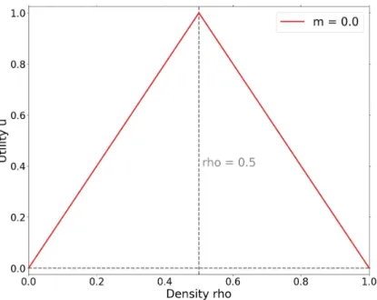
share the same utility function u(⇢) that depends on the agents density ⇢ in the neighborhood where they are located. We choose a triangular utility (see Fig. 2.1): agents experience zero utility if they are alone (⇢ = 0) or in full blocks (⇢ = 1), and maximum utility u = 1 in half-filled blocks (⇢ = 0.5). The collective utility U is

defined as the sum of all agents’ utilities, U = H PQ

q=1⇢qu(⇢q) and the average utility

˜

u per agent is ˜u = U/N .

Building upon past work on Schelling’s segregation model [Grauwin et al., 2009], we now mix two types of agents: "egoists", who act to improve their own, individual, utility, and a fraction p of "altruists", who act to improve the collective utility. Thus, egoists have as objective function the variation of their individual utility ∆u, while altruists consider the variation of the overall utility ∆U. The dynamics is the following: at each time step, an agent and a free site in another block are selected at random. The agent accepts to move to this new site only if its objective function strictly increases (note that the moving agent is taken into account to compute the density of the new block). Otherwise, it stays in its present block. Then, another agent and another empty site are chosen at random, and the same process is repeated until a stationary state is reached, i.e., until there are no possible moves for any agent.

2.3 Limiting cases: pure egoist or altruist

popula-tions

Authors in [Grauwin et al., 2009] computed analytically the stationary states of a homogeneous population of egoist or altruist agents. Altruists always reach the optimal

state, given by half filled (or empty) blocks and an average pure altruist utility ˜uA' 1.

In contrast, a pure egoist population collectively maximizes not U but an effective free energy that we have called the link L. The link is given by the sum over all blocks q

of a potential lq: L = Pqlq, where lq = P

Nq

nq=0u(nq/H), with Nq = H⇢q is the total

number of agents in block q. In the large H limit,

l(⇢q) ⇡ H

Z ρq

0

(22)

CHAPTER 2. COMPLEX DYNAMICS FROM A SIMPLE SOCIAL MODEL ₁₀

Figure 2.1 – Agent utility function: u(⇢) = 2⇢ for ⇢  0.5 and u(⇢) = 2(1 − ⇢) for ⇢ > 0.5.

The link may be interpreted as the cumulative of the individual marginal utilities gained by agents, as they progressively enter the blocks from a reservoir of zero utility. Its key property is that, for any move, ∆L = ∆u. Since egoists move only when their individual ∆u is positive, the stationary state is given by maximizing L over all possible

densities {⇢q} of the blocks, from which no further ∆u > 0 can be found. Analytical

calculations [Grauwin et al., 2009] show that this stationary state corresponds to crowded neighborhoods, far above the state of maximum average utility given by

⇢q = 1/2. For the case studied in this chapter, the stationary density is given by

⇢E = 1/

p

2, leading to a pure egoist utility ˜uE = 2(1 − ⇢E) ' 0.586 ⌧ 1. Numerical

simulations have confirmed these results, though the existence of many metastable

states around ⇢E ' 0.7 leads to fluctuations in the simulated final densities.

2.4 Mixing populations: qualitative picture

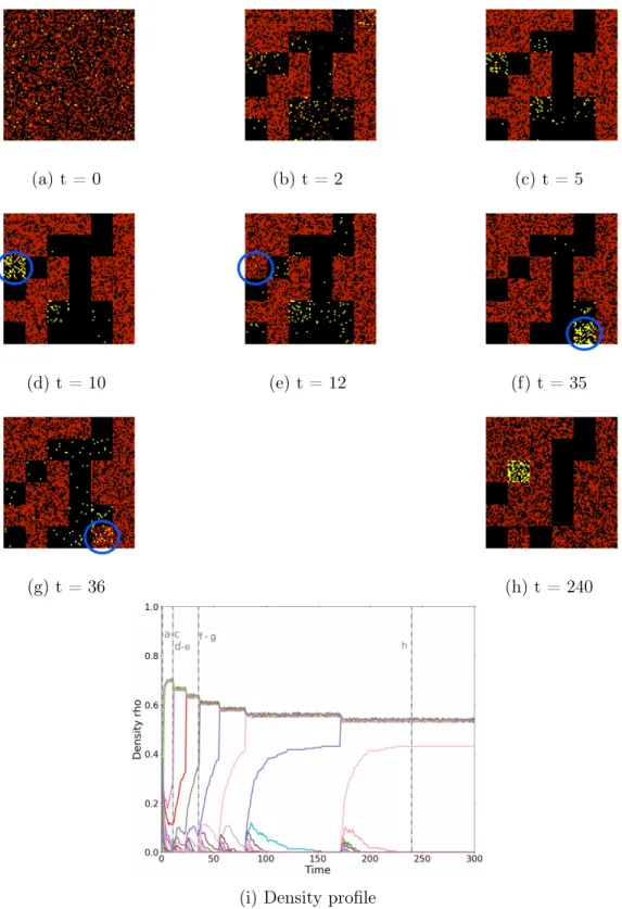
We now investigate how adding a fraction of altruists drives the system away from the frustrated pure egoist case to the optimal configuration observed in the pure altruist case. We find that, instead of a linear response, the system reaches the optimal state even at very low altruist concentrations (p < 0.01 in figure 2.2 a). To help understand-ing the origin of this strongly non-linear effect, the different panels of Fig. 2.3 illustrate the evolution of a small system (H = 225, Q = 36 and p = 0.04). Initially, altruists (yellow) and egoists (red) are distributed randomly in the blocks (a), which all have

a density ⇢ ' ⇢0 = 0.4. Then, blocks with the lowest densities are depleted by both

altruists and egoists that prefer districts with higher densities. At some point, when the block density increases, the behavior of the two kinds of agents diverge. Altruists "sacrifice" themselves and leave these high density blocks, moving to blocks with lower densities, as this increases the utility of their many (former) neighbors, leading to an

(23)

CHAPTER 2. COMPLEX DYNAMICS FROM A SIMPLE SOCIAL MODEL ₁₁

(a)

(b)

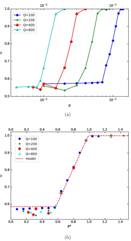
Figure 2.2 – Evolution of the average utility as a function of (a) the altruists’ fraction

p (note the log scale on the x-axis) and (b) the rescaled fraction p⇤

= 2pQ⇢0. We

take H = 200 and vary Q as shown. The fluctuations for low p⇤ values (before the

(24)

CHAPTER 2. COMPLEX DYNAMICS FROM A SIMPLE SOCIAL MODEL ₁₂ increase in global utility. On the other hand, egoists would loose individual utility by doing so, and therefore remain in these high density blocks which continue to feed on the remaining neighborhoods with ⇢ < 1/2. After a few iterations (Fig. 2.3b-c), selfish agents have gathered into "segregated" neighborhoods. This is the classical segregation observed in the pure egoist case [Grauwin et al., 2009], arising from the well studied amplification of density fluctuations. Note that all altruists have left the egoist blocks and gather into few blocks with lower densities (Fig. 2.3c) and then into a single neighborhood, whose density increases until it becomes attractive for egoist agents who "invade" it (Fig. 2.3d-e), while altruists leave it for other lower density blocks (Fig. 2.3e). The density of some of these new blocks then increases, allowing for successive egoist invasions (Fig. 2.3f-g). These migrations of egoist agents reduce the density of the overcrowded egoist blocks, increasing the overall utility. Eventually, the system reaches a stationary state in which no agent can move to increase its objective function (Fig. 2.3h).

2.5 Quantitative description

We now give a quantitative explanation of the decrease of egoist block densities and show that an altruist concentration p ' 1/Q is sufficient to drive the system towards the optimal state, ˜u = 1. To understand altruists’ dynamics, it is useful to replace their

dynamics by an equivalent egoist dynamics with a utility ualtr(⇢) that differs from the

original utility u(⇢). An exact mapping can be done in the following way. As mentioned

above, each altruist agent tries to maximize the global utility U = H PQ

q=1⇢qu(⇢q).

In contrast, an egoist agent acts to maximize the link function L = P_q`(⇢q), with

`(⇢q) given in Eq. (2.1). As a result, an altruist agent exactly behaves as an equivalent

egoist agent with a utility function ualtr(⇢) satisfying the relation

⇢u(⇢) = Z ρ 0 ualtr(⇢ 0 ) d⇢0 (2.2) since the resulting function to be maximized is the same. Differentiating this last equation, one finds

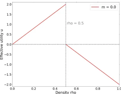
ualtr(⇢) = @$⇢ u(⇢)% @⇢ = ( 4⇢, _{for ⇢ } 1 2 2(1 − 2⇢), for ⇢ > 1 2 (2.3) This effective utility function for altruists is plotted on Fig. 2.4. Note that this ef-fective utility is not the one used to compute average or global utilities, it only helps

understanding altruists’ moves, since an altruist moves to a new block only if ualtr(⇢)

increases. Fig. 2.4 shows that altruists have a clear preference for blocks with densities just below 1/2. The large discontinuity at ⇢ = 1/2 arises because at this density the original utility function u(⇢) changes slope and starts to decrease. Then, an altruist moving from a block with ⇢ < 1/2 to a slightly more populated one with ⇢ > 1/2 induces a large decrease of total utility, since all its former neighbors loose utility (as the density of the initial block decreases) and so do its new neighbors, as the density of their block increases.

(25)

CHAPTER 2. COMPLEX DYNAMICS FROM A SIMPLE SOCIAL MODEL ₁₃

(a) t = 0 (b) t = 2 (c) t = 5

(d) t = 10 (e) t = 12 (f) t = 35

(g) t = 36 (h) t = 240

(i) Density profile

Figure 2.3 – Evolution of the city for p = 0.03, Q = 36 and H = 225. Panels (a-h) show the occupation of the different neighborhoods at different times. Egoists are represented in red, altruists in yellow, empty sites in black. (a) initial; (b) first steps; (c) usual segregation; (d-e): first invasion and altruist escape from the block surrounded in blue; (f-g): final invasion of the block surrounded in blue; (h): stationary state. In panel (i), each continuous line represents the evolution of the density of a single neighborhood. Vertical dashed lines show the times corresponding to panels (a-h).

(26)

CHAPTER 2. COMPLEX DYNAMICS FROM A SIMPLE SOCIAL MODEL ₁₄

Figure 2.4 – Effective utility function of altruistic agents.

Fig. 2.2b suggests that the transition towards the optimal state is continuous and takes place at an altruist concentration p ' 1/Q for all values of Q. This Q dependence is important, since in the thermodynamic limit (Q ! 1), the transition would take place at p ! 0. We now derive this result in a simple way by computing analytically the evolution of the average utility as a function of the altruist concentration p. Let’s start with very low altruist concentrations and assume that the initial dynamics is dominated by egoists, which form the usual Schelling’s overcrowded blocks, as observed above (Fig. 2.3c) and in previous work [Grauwin et al., 2009]. Therefore, we take

as starting point a city composed of nE egoist blocks with uniform density ⇢e =

⇢E > 1/2, such that ⇢E = (1 − p)Q⇢0/nE. Taking a uniform ⇢e value is justified

because any density fluctuation for ⇢e > 1/2 is rapidly wiped out by the dynamics,

as shown by the unique density of egoist blocks in Fig. 2.3i. Altruists can be initially somewhat scattered over the remaining blocks but, as their effective utility clearly shows (Fig. 2.4), they rapidly aggregate into a single block, leading to an altruist

density ⇢a= pQ⇢0 provided ⇢a< 1/2, or equivalently

p < phigh⌘

1

2⇢0Q

. (2.4)

The driving force for the transition are the relative values of agents’ utilities in egoist

and altruist blocks, respectively ue = uE = 2 − 2⇢E and ua = 2⇢a since ⇢a < 1/2

and ⇢E > 1/2. For very low p values, ⇢a is small, leading to ue > ua and the system

remains in the usual frustrated Schelling egoist state ˜u(p) ' ˜uE which is essentially

constant. When p reaches a value plowsuch that u(⇢a+1/H) > u(⇢E), a first egoist can

improve its utility by moving into the altruist block, whose density becomes ⇢a+ 1/H

(Fig. 2.3d-f). This gives :

plow ⌘ 1 − ⇢

E− 1/H

⇢0Q

, (2.5)

The density of the invaded block rapidly increases (Fig. 2.3e) and eventually reaches 1/2. At this point, altruists’ effective utility becomes negative, pushing them to leave

(27)

CHAPTER 2. COMPLEX DYNAMICS FROM A SIMPLE SOCIAL MODEL ₁₅ for other lower density blocks (Fig. 2.3f). As previously, altruists gather in another

single block of identical density ⇢a = pQ⇢0. The invasion has led to a slight decrease

of the density of egoist blocks to ⇢e< ⇢E, and therefore to a slight increase of egoists’

utility, ue= u(⇢e) > u(⇢E). Successive invasions of the block partially filled by altruists

are possible until ⇢edecreases down to the value ⇢⇤e such that u(⇢

⇤

e) = u(⇢a+1/H). This

leads to ⇢⇤

e = 1 − pQ⇢0− 1/H (⇢⇤e > 1/2 as long as p < phigh). The equality of utilities

implies ˜u(p) = u(⇢a) = 2pQ⇢0+ 2/H. When p = phigh, the final (lowest) egoist density

reaches the optimal value ⇢⇤

e = 1/2 and no further improvement in average utility

is possible: ˜u(p) = 1 (to simplify the discussion, we ignore here corrections of order 1/H that depend on the parity of H). This description remains valid for larger altruist concentrations, the only difference being that, at the end, the additional altruists form

stable blocks with densities ⇢a= 1/2.

In summary, the evolution of the average utility ˜u follows: 8 > < > : ˜

u(p) = 2 − 2⇢E for p  plow

˜

u(p) = 2pQ⇢0+ 2/H for plow  p  phigh

˜

u(p) = 1 _{for p ≥ p}high

(2.6)

Our analysis predicts that plotting ˜u as a function of the rescaled altruist proportion

p⇤ _{= p/p}

high = 2pQ⇢0 should lead to a universal transition starting at p⇤ = 2 − 2⇢E '

0.586 and ending at p⇤

= 1. Simulations perfectly confirm our calculations (Fig. 2.2b).

2.6 Discussion

Our model illustrates the complexity of the dynamics produced by two types of agents, even when they follow simple rules. Introducing altruists into a population dominated by egoists increases the average utility much more rapidly than expected from a lin-ear projection. The interplay between the different behaviors leads to complex "cat-alytic" phenomena. By catalytic, we mean that altruists are not "consumed" once they coordinate egoists, and can continue to help egoists finding the optimal config-uration indefinitely. The global utility increase per altruist can be computed easily:

δUaltr ⌘ (U(p)−U(p = 0))/NA' (1−0.56)⇢0QH/(p⇢0QH) = 0.44/p. When p = 1/Q,

δUaltr ' 0.44Q. Each altruist induces a utility change proportional to the system size,

which becomes infinite for infinite systems.

Interestingly, while the stationary state of a system composed of a single type of agents (either egoists or altruists) can be mapped to an equilibrium state, this is no longer the case when including two types of agents, except if some restrictive conditions are met [Grauwin et al., 2009]. In a thermodynamic analogy, the utility function can be mapped (in the zero temperature limit considered here) to a chemical potential, as shown in [Lemoy et al., 2012], when a single type of agents is present. If a system with both egoist and altruist agents could be mapped to an equilibrium system, chemical

potentials could be defined as µe(⇢a, ⇢e) = u(⇢a+⇢e) and µa(⇢a, ⇢e) = ualtr(⇢a+⇢e). As

chemical potentials derive from a free energy, their cross derivatives would be equal,

@µe/@⇢a = @µa/@⇢e, leading to u0(⇢) = u0altr(⇢). This equality is not satisfied as seen

(28)

CHAPTER 2. COMPLEX DYNAMICS FROM A SIMPLE SOCIAL MODEL ₁₆ We are well aware that simple models do not allow to draw any rigorous conclusion about what is going on in the real world [Venturini et al., 2015, Ostrom, 2010, Jensen, 2018]. While Schelling’s segregation model neatly shows that one cannot logically deduce individual racism from global segregation, it may well be that for some towns racism is one cause of segregation, for some others not; at any rate the reasons behind urban segregation are far more complex than those that any simple model can come up with. Simple models can be helpful to analyze some interesting phenomena, the origin of which may be obscured in more complicated realistic settings. Ours may help thinking about the effectiveness of coordination by an infinitesimal proportion of altruist agents, but it cannot be directly applied to real systems. Real agents do not behave like these virtual robots: they are able to put their actions into context, to anticipate the behavior of the others and moreover, they disagree about what is the social "optimum" [Jensen, 2018, Latour, 1988].

In this chapter we discussed the limitations of simple statistical physics models of society and the complex dynamics which can emerge from simple simulated models. In the next chapter, we explore the dynamics of a real world system using the dataset of Vélo’v users, a bike sharing system based in Lyon. We will illustrate the advantage of using temporal data and the difference between global evolution of the system and individual evolutions of its units.

(29)

3

Dynamics of Bike Sharing System Users

3.1 Introduction

Bike Sharing Systems (BSS) have been developing rapidly all over the world in the last decades, being now present in more than 500 cities. The number of studies of BSS has followed a similar pattern, focusing on 3 topics : quantifying BSS characteristics, describing users’ socio-demographic profiles and evaluating its impacts on environment and public health.

The automatic recording of BSS activities has allowed a quantitative description of many BSS characteristics: Circadian and monthly activity patterns (see [Borgnat et al., 2011, Côme et al., 2014]), average speed ([Jensen et al., 2010]), patterns of bicycle flows over the cities (see [Côme et al., 2014, Jensen et al., 2010, Borgnat et al., 2011, Borgnat et al., 2013]) and influence of weather conditions ([Borgnat et al., 2011]). The knowledge derived from these studies, especially on bicycle flows between stations (see [Côme et al., 2014, Tran et al., 2015]) and the prediction of bike reallocation schedules ([Zhang et al., 2016]), can help the management of station balancing (see [Singla et al., 2015, Côme et al., 2014, Côme and Oukhellou, 2014]), one of the main financial challenges of BSS ([Yang et al., 2011]).

Socio-demographics profiles of BSS users differ generally from the overall cities demographics. Studies carried out in Europe and North America (see [Beecham and Wood, 2014, LDA-Consulting, 2012, Ogilvie and Goodman, 2012, Shaheen et al., 2012, Fuller et al., 2011, Raux et al., 2017]) have shown that users are more likely to be young, male, with a high level of education and living in the city center.

Finally, several studies have described the impact of BSS policies on environment and public health (see [Pucher and Buehler, 2012]). [Shaheen et al., 2010, Shaheen et al., 2011] have listed the benefits of BSS: Emission reductions, individual financial savings, physical activity benefits, reduced congestion and facilitation of multimodal transport connections. Yet, other studies question the real impact of BSS on some of the latter. Notably [Shaheen et al., 2012] showed the relatively low impact on people favorite mode of transportation. In particular [Fishman et al., 2013, Midgley, 2011, LDA-Consulting, 2012, Buttner et al., 2011] exhibited, for several cities in Europe and Canada the low substitution rates from car usage to BSS. Most BSS riders are indeed people who used to walk and take public transportation.

(30)

CHAPTER 3. DYNAMICS OF BIKE SHARING SYSTEM USERS ₁₈ Among all the research axes cited, questions remain on the commitment of BSS subscribers in the long term. This is due to the lack of accurate trip datasets over long periods of time, as mentioned in [Fishman et al., 2013]. Some articles have tried to characterize travel behaviors using surveys, such as [Guo et al., 2017, Raux et al., 2017]. But the temporal evolution of users has never been deeply investigated. This is the reason why in this chapter we approach BSS travel behaviors and usage rates under the temporal angle. We address questions related to BSS sustainability, such as : how long do users remain active over the years ? Does their activity increase, decrease or remain stable? Do these trajectories depend on their level of activity? These questions are addressed using a five years long dataset covering about 150,000 long-term distinct users, among which 13,358 have stayed in the system for the whole period. We follow previous work on Lyon’s BSS, Vélo’v, by [Vogel et al., 2014] which, using a single year dataset (2011), characterized users according to their intensity and frequency of uses at different time scales (day, week, month and year). This work found 9 classes of users, ranging from ’extreme users’, that use Vélo’v twice a day on average to ’sunday cyclists’, who only use the system a few week-ends per year. Using a single year dataset to classify users has however two main limitations. Firstly, there is no way to distinguish between two possible interpretations for a user that appears to be very active from September to December. This could correspond either to (a) someone arriving in town in September that remains very active for the months/years to come or (b) someone who for an unknown reason uses the system only in those months. The second limitation arises from the impossibility to test the stability of users’ characteristics over years, which would allow to interpret them as real user properties. For example, do users classified in 2011 as ’sunday cyclists’ retain this characteristic over the years? Have they only used Vélo’v in this way in 2011 or is this pattern a more personal - and stable - use of the system that lasts for longer periods? The work presented in this chapter is one of the first giving a detailed description of how different segment of customers use Vélo’v over years. A recent article from [Jain et al., 2018] highlighted the lack of temporal analysis on BSS’ users and importance of tracing longitudinal usage trends. Our study could open the way to the establishment of a methodology to dynamically assess impact of BSS policies and other transportation facilities on different segment of users.

After presenting our 5-years dataset in Section 3.2, we start by describing the overall system stability. We, then, show the heterogeneous individual trajectories masked by this overall system stability in Section 3.4. Finally, we compute in section 3.5 user classes using a similar approach to [Vogel et al., 2014] and break down individual evolutions from section 3.4 using the classes we computed.

3.2 Dataset

The Vélo’v program started in 2005 in Lyon, France. The Vélo’v network now has 340 stations, where roughly 4000 bicycles are available. The stations are in the street and can be accessed at anytime (24/7) for rental or return. More information about the history of Vélo’v and the deployment of stations can be found in [Borgnat et al., 2011]. The dataset used in this chapter records all bicycle trips from 2011/01 to 2015/12 for the Vélo’v system. It contains more than 38 million trips made by more than 3.8

(31)

CHAPTER 3. DYNAMICS OF BIKE SHARING SYSTEM USERS ₁₉ million users. Each trip is documented with starting and ending times, duration, a user ID code and a tag describing the class of user (year-long subscriber, weekly or daily subscription, maintenance operation, etc). Data are filtered according to the process used in [Vogel et al., 2014], keeping only year-long users and eliminating any anomalies. This leads to a subset of the original population containing 147,354 long-term users. For each person, we count years from the first active day: For example,

a user appearing in the records for the first time on March 16th_{, 2011 will end the}

first adapted year on March 15th_{, 2012. To avoid boundary artifacts for users that are}

active over several years, we stop recording trips at the anniversary date in 2015, even if there are recorded trips later in 2015.

Note that our elementary unit of analysis is therefore the ’person-year’, i.e. the vector of 21 features for each user and each year. One person can therefore appear several times (up to 5) and change group from year to year. One could adopt a different point of view, using persons as the entities and computing a single vector for each of them, averaged over their whole period of activity. This would have two drawbacks: masking the single user trajectories over the years and comparing vectors computed over different periods (from 1 to 5 years). Comparing the third and fourth columns of Table 3.3 shows that using the ’person-year’ or the ’person’ as the basic entity leads to roughly the same proportions for the different classes. We then retain the ’person-year’ description, which allows studying users’ trajectories.

3.3 Overall evolution

We first analyze the global system evolution over the 5 years. Table 3.1 shows that there is a steady increase in the number of users and trips. However, the average number of trips per user remains remarkably stable around 92 trips/year, despite the large variability (standard deviation larger that the average). A similar general temporal trend is found in [Jain et al., 2018].

3.4 Individual evolutions

The overall system stationarity (slow increase of user numbers) hides a great variability at the individual level that can be uncovered only using long-term datasets at the individual level as ours. Every year, there is a strong user renewal, as the majority of users leave the system after their first year of activity and are replaced by a greater

Year 2011 2012 2013 2014 2015

Active Users 50,393 55,896 61,806 70,068 76,511

Trips 4,702,498 5,138,971 5,576,973 6,625,090 7,044,707

Trips per user 93.3 91.9 90.2 94.5 92.0

Median trips per user 45 46 45 49 46

Standard Deviation 125.6 122.8 120.7 123.8 123.8

(32)

CHAPTER 3. DYNAMICS OF BIKE SHARING SYSTEM USERS ₂₀

Figure 3.1 – Progressive renewal of users over the years. For each year, the box height represents the total number of users and the colors the year users have entered the system. For example, in 2015, 34.4% of users are new to the system, while 18% started in 2011.

number of new users. Figure 3.1 shows that every year the new users represent around 35% of the total. Then, they progressively leave the system, in a quite predictable way: They represent 26-28% of users the year after and 11-12% two years later. The only exception is the 2011 cohort, which by lack of data over the previous years, also includes users that entered the system before 2011.

3.4.1 Most users leave the system after one year

Analyzing user activity over calendar years as in Figure 3.1 is confusing, since users enter the system at any time during the year. To follow individual evolutions, we have to shift the different starting dates to a common origin using ’adapted’ years as explained above.

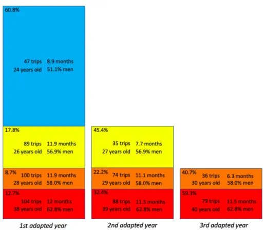
Figure 3.2 shows that a large majority of users (60.8%, blue rectangle) quit after a single year of practice. These users are significantly younger than more loyal users (24 years old against 31), more likely women (51.1% of men compared to 59.1%) and less active: their median number of trips is 47, to be compared to 91. This low activity is mainly explained by a shorter time span of their activity (median close to 9 months instead of the whole year). This means that many of them stop using the system before the 12-month validity of their subscription, because they leave Lyon, buy a bike, change job. . .

Almost 20% of users stay in the system for 2 years (yellow rectangles in figure 3.2). Note that their activity is significantly lower than that of more loyal users, that will

stay in the system for 3 or 4 years (89 trips against 100, p-value < 2.2 ⇤ 10−16_{). In this}

case, this reduced activity cannot be explained by a shorter activity time span. These users are consistently less active over the whole year, a feature that allows to predict a higher chance of quitting the system the following year as we will check below. When

(33)

CHAPTER 3. DYNAMICS OF BIKE SHARING SYSTEM USERS ₂₁

Figure 3.2 – Percentages of users leaving the system at the end of different adapted years. For each group of users is given the median number of trips per year, the median number of active months, the median age and the percentage of men. For example ’Blue users’ stopped at the end of their first adapted year, after a median number of 8.9 months of activity. They represent 60.8% of first year users. They had a median number of trips during that year of 47, a median age of 24 years old and 51.1% were men. Yellow users stopped at the end of their second adapted year. They had a median number of trips during their first year of 89 and during their second year of 35. They stopped after a number of 7.7 active months during their second year. these users reach their second (and last) active year, their activity becomes quite similar to the blue users, as their time span is reduced to 7.7 months and their activity much lower than in their first year (35 trips instead of 89).

Almost 9% of users stay in the system for 3 years (orange rectangles in figure 3.2). Again, their activity, even two years before leaving the system, is significantly lower

than that of more loyal users (100 trips against 104, p-value < 2.2 ⇤ 10−16_{). This}

activity progressively diminishes over the years, reaching a very low value on the third and final year (36 trips over 6.3 months).

Finally, 12.7% of users stay in the system for at least 4 years (red rectangles in figure 3.2). Their activity is consistently higher than average, and these users are older and more often men. Their activity also progressively diminishes over the years, a feature that we study in more detail below.

The most striking result is the high proportion (60.8%) of users that quit after a single year of practice (called ’leavers’ hereafter). To the best of our knowledge, this surprising figure was previously unknown. It is worth noting however that this figure

(34)

CHAPTER 3. DYNAMICS OF BIKE SHARING SYSTEM USERS ₂₂

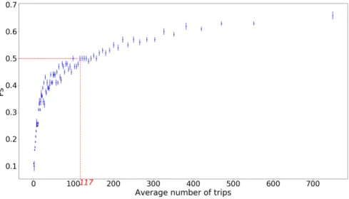
Figure 3.3 – Probability to stay in the system at the end of an adapted year (Ps) as

a function of the average number of trips during that year. When activity reaches

110-120 trips per year, users are more likely to stay (Ps≥ 0.5). Each point represents

an average of Ps over 2500 person-years.

might be slightly overestimated. The reason is that users are identified through the ID of different cards, the most common being Velo’v own card (30.3% of the users), public transportation card (Tecely, 59.7%) and train card (Oura, 5.2%). The point is that the Tecely cards have to be renewed every 5 years. In some (uncontrolled) cases, this leads to a change of ID, which our analysis interprets as if the user had left the system and another had entered it. To estimate the proportion of incorrectly labeled exits from the system, we note that only 46.6% of Velo’v cards users give up after one year, the corresponding figure being 61.3% for Tecely users. As Velo’v cards do not go through the yearly renewal process, this percentage could represent a lower bound on the ’leavers’ proportion, if we assume that the proportion of leavers does not depend on the card used, which seems unlikely as using the specific Velo’v card suggests a higher loyalty. To obtain another estimation, we may assume that all renewed Tecely cards (20% per year) change their ID. This would mean that the 61.3% figure is an overestimation of the real figure (61.3 - 20)/0.8 = 51.6%. These estimates converge to a proportion of leavers between 50 and 55%.

We noted above that the loyalty of users was correlated to their activity. Figure 3.3 shows the general trend over all users. It confirms that the higher the intensity of use,

the higher the probability Ps to stay in the system. This result can help predicting

users’ loyalty.

3.4.2 Long-term users are older, more likely men and more

urban than average

Let us now focus on the most loyal users, the 25,963 users that have been active for at least 3 years, which we now call ’long-term’ users. Comparing them to those that leave after a single year reveals interesting facts about their specific characteristics.

(35)

CHAPTER 3. DYNAMICS OF BIKE SHARING SYSTEM USERS ₂₃

Ages N % men % long-term users % men in long-term users

13-22 11,231 54.8 25.2 60.5 23-32 18,081 54.5 31.6 59.3 33-42 9,572 62.6 49.8 65.7 43-52 6,413 57.6 57.3 58.8 53-62 3,774 55.9 59.6 57.0 63-72 1,194 65.1 64.7 67.4

Table 3.2 – Description of long-term users characteristics

They are older (median age 35, against 24, p-value < 2.2 ⇤ 10−16_{), more likely men}

(men proportion 62.9% against 49.9%, p-value < 2.2 ⇤ 10−16_{) and live within the}

Lyon-Villeurbanne urban area (85.3% against 81.7%, p-value < 2.2 ⇤ 10−16₎

Table 3.2 shows the proportions of long-term users for different 10-years slices. Clearly, loyalty steeply increases with age, from 25.2% for 13-22 years old users up to 64.7% for 63-72 years old users. Men are over-represented among the long-term users for all ages, but the difference is highly significant among younger users. It would be interesting to understand why there are (comparatively) so few young women among the most loyal BSS users.

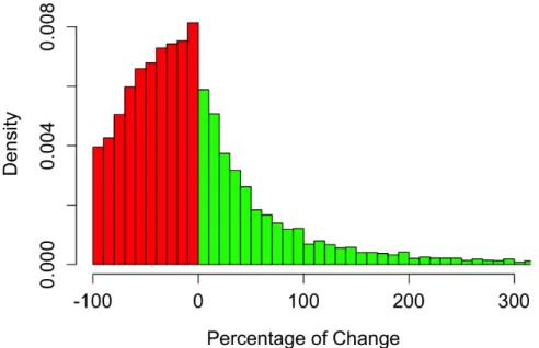
Finally, we study how long-term users change their activity over the years. For each user, we computed the percentage of change in the number of trips per year from one year to another. Figure 3.4 shows that only one quarter (26.5%) maintain their number of trips within a ±20% range. Roughly two-thirds (61.8%) users lower their activity, almost halving it (median decrease 42.3%). The remaining third increases its activity (median increase 42.6%). The median evolution of long term users is a decrease of activity by 16.3%.

We now apply a k-mean algorithm to the set of person-years to describe to finer level the evolution of users, we discuss the number of clusters and compare our findings to the results of [Vogel et al., 2014], in which the authors used the same methodology on a 1-year dataset.

3.5 Classes of users

In this section, we compute users classes on our 5 years dataset, using a similar ap-proach to [Vogel et al., 2014], and offer a brief description of them. Computing these classes allows us to compare our results to the one found in [Vogel et al., 2014]. This comparison illustrates the effect of temporality on users classification accuracy.

3.5.1 Computing users classes

From this dataset, we compute the same 21 normalized features characterizing the activity as in [Vogel et al., 2014]. For each person, these features quantify the intensity and regularity of use over the year (14 features) and the week (7 features).

(36)

CHAPTER 3. DYNAMICS OF BIKE SHARING SYSTEM USERS ₂₄

Figure 3.4 – Density distribution of percentage of change in the number of trips per year from one year to another. Percentages are computed for each user that remained active for at least 3 years.

during which users traveled at least once, and normalised dividing by 1.5 times the interquartile range of the distribution for all users (equal to the difference between the lower and upper quartile of the distribution).

• trips day1 − 5, number of trips per week day. Days are ranked from one to five, day 1 being the day with the highest number of trips and day 5 the day with the lowest number of trips. trips saturday, average number of trips made on Saturdays. trips sunday, average number of trips made on Sundays. These seven features are normalized over a total sum unity over the week.

• trips year, total number of trips made over the adapted year, normalized dividing by 1.5 times the interquartile range of the distribution for all users (i.e. the difference between the lower and upper quartile of the distribution).

• trips month1 − 12, number of trips per month, normalized to a total sum unity, months are ranked from one to twelve, month 1 being the month with the highest number of trips and month 12 the month with the lowest number of trips. As explained in [Vogel et al., 2014], there is some correlation and redundancy between intensity and regularity features. Nevertheless, a simple K-means clustering method (see, e.g., [MacKay, 2003]) is used, coupled with statistical appraisal and careful analysis of the results, as our main intent is to create and interpret a relevant typology, not to find well-defined, pre-existing, classes. Also, we prefer to use the original variables instead of PCA axes, because this makes the interpretation of the obtained classes straightforward.

To choose the number of clusters, we studied as [Vogel et al., 2014] the partitions obtained when choosing from three to twelve clusters. However, as shown on figure

(37)

CHAPTER 3. DYNAMICS OF BIKE SHARING SYSTEM USERS ₂₅

Figure 3.5 – Visualization of the users-year on the two main axis given by principal component analysis (PCA)

3.5, there is a continuum distribution of users-year and therefore no clear separation to split the clusters. Moreover we also computed the Akaike Information Criteria (AIC) for the different number of clusters k. The AIC is defined as follow:

AIC(k) = −2L(k) + 2q(k) (3.1)

Where −L(k) is the negative maximum likelihood for k clusters and q(k) is the number of parameters of the model with k clusters. Hence, the AIC represents the trade-off be-tween a model which clusters well the data (given by the likelihood) and the complexity

of the model. The optimal number of clusters k is in theory argmink[−2L(k) + 2q(k)].

However after plotting AIC(k) (Figure 3.6), we observe that there is no clear knee showing an optimal value.

Hence, we chose nine clusters for two reasons. Firstly, we found that as in [Vogel et al., 2014], this number of clusters represents the best compromise between a reduced but rich enough description (differentiating for example week-end users from week users), without introducing uninformative clusters. Secondly, this number allows a simple comparison of our results with the study from 2014.

A detailed description of the nine classes is given in Table 3.3 and Figure 3.7.

3.5.2 User Classes

The nine classes correspond to different profiles of use. There are 6% of ’one-off’ users, who make on average only 3 trips per year, generally the same month and then disappear from the database. Another almost 12% of users are mainly active in week-ends, either for shopping (Saturdays) or leisure (Sundays) (second line of Table 3.3). The last 6 lines of Table 3.3 represent users that show a regular activity over the year and differ mainly by their intensity of use, from twice a month (regular0 class, gathering 27% of users) to nearly twice a day (regular5, 1% of users). The part-time class is quite peculiar: we will show below that it can be interpreted as the class where users end up for the last year of activity.

3.6 Evolution of user classes

This section answers to the question: what are the differences between stable users in terms of practice, i.e. what is the dynamics of stable users within the classes?

Understanding the complex dynamics of social systems with diverse formal tools

HAL Id: tel-02456654

https://tel.archives-ouvertes.fr/tel-02456654

Understanding the complex dynamics of social systems

with diverse formal tools

Jordan Cambe

To cite this version:

Acknowledgements

Abstract

Résumé

Contents

List of Figures

List of Tables

1

Introduction

1.1

An Overview of Network Science

1.1.1

Static Complex Networks

1.1.2

Temporal Complex Networks

1.1.3

Networks in Social Sciences

1.2

Statistical Physics Models

1.3

Machine Learning

1.4

Contributions and Chapter Outline

1.5

List of PhD Publications

2

Complex Dynamics From a Simple Social Model

2.1

Introduction

2.2

Description of the model

2.3

Limiting cases: pure egoist or altruist

popula-tions

2.4

Mixing populations: qualitative picture

2.5

Quantitative description

2.6

Discussion

3

Dynamics of Bike Sharing System Users

3.1

Introduction

3.2

Dataset

3.3

Overall evolution

3.4

Individual evolutions

3.4.1

Most users leave the system after one year

3.4.2

Long-term users are older, more likely men and more

urban than average

3.5

Classes of users

3.5.1

Computing users classes

3.5.2

User Classes

3.6

Evolution of user classes