HAL Id: hal-01856950
https://hal.archives-ouvertes.fr/hal-01856950
Submitted on 13 Aug 2018
HAL is a multi-disciplinary open access
archive for the deposit and dissemination of
sci-entific research documents, whether they are
pub-lished or not. The documents may come from
teaching and research institutions in France or
abroad, or from public or private research centers.
L’archive ouverte pluridisciplinaire HAL, est
destinée au dépôt et à la diffusion de documents
scientifiques de niveau recherche, publiés ou non,
émanant des établissements d’enseignement et de
recherche français ou étrangers, des laboratoires
publics ou privés.
Jean-Marc Ginoux, Jaume Llibre
To cite this version:
Jean-Marc Ginoux, Jaume Llibre. Canards Existence in Memristor’s Circuits. Qualitative Theory of
Dynamical Systems, SP Birkhäuser Verlag Basel, 2016, 15 (2), pp.383 - 431.
�10.1007/s12346-015-0160-1�. �hal-01856950�
The aim of this work is to propose an alternative method for determining the condition of existence of “canard solutions” for three and four-dimensional singularly perturbed systems with only one fast variable in the folded saddle case. This method enables to state a unique generic condition for the existence of “canard solutions” for such three and four-dimensional singularly perturbed systems which is based on the stability of folded singularities of the normalized
slow dynamics deduced from a well-known property of linear algebra. This
unique generic condition is perfectly identical to that provided in previous works. Application of this method to the famous three and four-dimensional memristor canonical Chua’s circuits for which the classical piecewise-linear characteristic curve has been replaced by a smooth cubic nonlinear function according to the least squares method enables to show the existence of “canard solutions” in such Memristor Based Chaotic Circuits.
Key Words: Geometric singular perturbation theory, singularly perturbed
dy-namical systems, canard solutions.
1. INTRODUCTION
As recalled by Fruchard and Sch¨afke [20, p. 435]: “In the late 1970s, under the leadership of George Reeb, a group of young researchers, Jean-Louis Callot, Francine and Marc Diener, Albert Troesch, Emile Urlacher and then, Eric Benoˆıt and Imme van den Berg, based in Strasbourg some in Oran and others in Tlemcen were given as research program to develop methods for “non-standard analysis1” for the study of singular perturbation problems. Georges Reeb had proposed to introduce a particular control parameter a in the original van der Pol’s equation [45].
ε¨x + (1− x2) ˙x + x = a
The study of this equation has led this group to discover surprising so-lutions, which they named “ducks2”. Van der Pol relaxation oscillator
is considered as the paradigm of slow -fast systems, i.e. two-dimensional 1For more details see Robinson [38] and Nelson [34].
2Canards in French.
singularly perturbed system with one slow variable and one fast. It is well-known that for the control parameter value a = 1, a Hopf bifurcation takes place in this system3. So, as expected by this group of researchers, by
setting ε constant, one would make the amplitude of the periodic solution (limit cycle) change very fast for values of a near (just below) 1. But, the results exceeded their expectations: at one critical value a = 0.9987404512 a very small change of this parameter’s value produced an amplitude drop of about 80 %.
According to Marc Diener [13, p. 38]: “It was as if the existence of medium size solutions would be a “canard4”! Canard is now the name of a type of solution of a slow-fast differential system, to which the above “miss-ing” medium-size solutions belong, that had previously been ignored.”. An-other interpretation of the denomination “canard” also given by Diener [13, p. 45] in the the same article, is that the periodic solution resembles, for this critical parameter value, to a duck (See Fig. 1.).
FIG. 1. “Canard cycle” of the Van der Pol equation, Diener [13, p. 45].
In the beginning of the eighties, Benoˆıt and Lobry [5], Benoˆıt [6] and then Benoˆıt [7] in his PhD-thesis studied canard solutions in R3. In the article entitled “Syst`emes lents-rapides dans R3 et leurs canards,” Benoˆıt [6, p. 170] proved the existence of canards solution for three-dimensional singularly perturbed systems with two slow variables and one fast variable while using “Non-Standard Analysis”according to a theorem which stated that canard solutions exist in such systems provided that the pseudo singu-3See Callot et al. [10], Benoˆıt et al. [2], Benoˆıt et al. [3], Benoˆıt [4] and Ginoux et al.
[21].
4Canard = false report, from the old-French “vendre un canard moiti´e” (Sell the half
lar point5of the slow dynamics, i.e., of the reduced vector field is of saddle
type.
Nearly twenty years later, Szmolyan and Wechselberger [41] extended “Geometric Singular Perturbation Theory6” to canards problems in R3
and provided a “standard version” of Benoˆıt’s theorem [6]. Very recently, Wechselberger [47] generalized this theorem for n-dimensional singularly perturbed systems with k slow variables and m fast (Eq. (1)). The method used by Szmolyan and Wechselberger [41] and Wechselberger [47] require to implement a “desingularization procedure” which can be summarized as follows: first, they compute the normal form of such singularly perturbed systems (see Eq. (28) for dimension three and Eq. (48) for dimension four) which is expressed according to some coefficients (a and b for dimension three and ˜a, ˜b and ˜cj for dimension four) depending on the functions
defin-ing the original vector field (1) and their partial derivatives with respect to the variables. Secondly, they project the “desingularized vector field” (originally called “normalized slow dynamics” by Eric Benoˆıt [6, p. 166]) of such a normal form on the tangent bundle of the critical manifold. Finally, they evaluate the Jacobian of the projection of this “desingularized vector field” at the folded singularity (originally called pseudo singular points by Jos´e Arg´emi [1, p. 336]. This leads Szmolyan and Wechselberger [41, p. 427] and Wechselberger [47, p. 3298] to a “classification of folded
singulari-ties (pseudo singular points)”. Thus, they show that for three-dimensional
singularly perturbed systems such folded singularities is of saddle type if the following condition is satisfied: a < 0 while for four-dimensional singu-larly perturbed systems such folded singularities is of saddle type if ˜a < 0.
Then, Szmolyan and Wechselberger [41, p. 439] and Wechselberger [47, p. 3304] establish their Theorem 4.1. which state that “In the folded saddle
and in the folded node case singular canards perturb to maximal canard for sufficiently small ε”. However, in their works neither Szmolyan and
Wech-selberger [41] nor WechWech-selberger [47] do not provide (to our knowledge) the expression of these constants (a and ˜a) which are necessary to state the
existence of canard solutions in such systems.
So, the aim of this work is first to provide the expression of these con-stants and then to show that they can be directly determined starting from the normalized slow dynamics and not from the projection of the “desin-gularized vector field” of the normal form. This method enables to state a unique “generic” condition for the existence of “canard solutions” for such three and four-dimensional singularly perturbed systems which is based on the stability of folded singularities of the normalized slow dynamics deduced from a well-known property of linear algebra. This unique
condi-5This concept has been originally introduced by Jos´e Arg´emi [1]. See Sec. 2.7. 6See Fenichel [14, 15, 16, 17], O’Malley [35], Jones [29] and Kaper [30].
tion which is completely identical to that provided by Benoˆıt [6] and then by Szmolyan and Wechselberger [41] and finally by Wechselberger [47] is “generic” since it is exactly the same for singularly perturbed systems of dimension three and four with only one fast variable. So, it provides a path to many applications.
In the very beginning of the seventies, Leon Chua [11] considered the three basic building blocks of an electric circuit: the capacitor, the resistor and the inductor as well as the three laws linking the four fundamental circuit variables, namely, the electric current i, the voltage v, the charge
q and the magnetic flux φ. He thus concluded from the logical as well as
axiomatic points of view, that it is necessary, for the sake of completeness, to postulate the existence of a fourth circuit element to which he gave the name memristor since it behaves like a nonlinear resistor with memory. On April 30th 2008, Stan Williams and co-workers [40] announced in the
journal Nature that the missing circuit element, postulated thirty-seven years before by Leon Chua has been found [23]. Since, the memristor has been subject to many studies and applications [12, 36]. More particu-larly, memristor-based circuits have been used by Itoh and Chua [27, 28], Muthuswamy and Kokate [31], Muthuswamy [32], Muthuswamy and Chua [33] and Fitch et al. [18, 19] to construct dynamical systems whose solu-tions exhibit chaotic and hyperchaotic behavior [18].
In a paper entitled “Duality of Memristors Circuits”, Itoh and Chua [28, p. 1330001-15] gave the memristor canonical Chua’s circuit equation (69) in the three-dimensional flux-linkage and charge phase space. Differentiating this Eq. (69) with respect to time they obtained memristor-based canonical Chua’s circuit equation (73) in the four-dimensional current-voltage phase space7. In both cases, the φ− q characteristic curve of these circuits has
been represented by a piecewise-linear function (Eq. (40) in Itoh and Chua [27, p. 3189] and Eq. (70) in Itoh and Chua [28, p. 1330001-15]). In their works, Itoh and Chua [27, 28] have shown that the dynamical systems modeling such circuits possess at least one eigenvalue with a large negative real part. This specific feature is of great interest since it enables to consider memristor-based canonical Chua’s circuits as slow-fast dynamical systems. So, there exists in the phase-space a slow manifold on which trajectories, solution of the dynamical system modeling the memristor circuit, evolve slowly and toward which nearby orbits contract exponentially in time in the normal directions.
For these memristor-based canonical circuits Itoh and Chua [27, 28] have used a classical piecewise-linear function for the φ− q characteristic curve. However, Muthuswamy [32] and Fitch et al. [18] have proposed to replace 7Let’s notice that Eq. (73) corresponds exactly to what Itoh and Chua [27, p.
3188] have called in their previous paper on “Memristor Oscillators” the fourth-order memristor-based canonical Chua’s circuit equation (35).
this piecewise linear characteristic curve by a smooth cubic nonlinear func-tion. This enables to exhibit the existence of generic “canard solutions” in such Memristor Based Chaotic Circuits.
The outline of this paper is as follows. In Sec. 2, definitions of singularly perturbed system, critical manifold, reduced system, “constrained system”, canard cycles, folded singularities and pseudo singular points are recalled. The method proposed in this article is presented in Sec. 3 & 4 for the case of three and four-dimensional singularly perturbed systems with only one
fast variable. Existence of canard solution for the third and fourth-order
Chua’s memristor is established according to this method in Sec. 5 & 6.
2. DEFINITIONS
2.1. Singularly perturbed systems
According to Tikhonov [43], Pontryagin [37], Jones [29] and Kaper [30]
singularly perturbed systems are defined as:
⃗
x′= ε ⃗f (⃗x, ⃗y, ε) , ⃗
y′= ⃗g (⃗x, ⃗y, ε) . (1)
where ⃗x∈ Rk, ⃗y ∈ Rm, ε ∈ R+, and the prime denotes differentiation with respect to the independent variable t′. The functions ⃗f and ⃗g are
assumed to be C∞ functions8 of ⃗x, ⃗y and ε in U× I, where U is an open
subset ofRk× Rmand I is an open interval containing ε = 0.
In the case when 0 < ε ≪ 1, i.e. ε is a small positive number, the variable ⃗x is called slow variable, and ⃗y is called fast variable. Using Landau’s notation: O (εp) represents a function f of u and ε such that f (u, ε)/εp is bounded for positive ε going to zero, uniformly for u in the
given domain.
In general we consider that ⃗x evolves at an O (ε) rate; while ⃗y evolves
at an O (1) slow rate. Reformulating system (1) in terms of the rescaled variable t = εt′, we obtain ˙ ⃗ x = ⃗f (⃗x, ⃗y, ε) , ε ˙⃗y = ⃗g (⃗x, ⃗y, ε) . (2)
The dot represents the derivative with respect to the new independent variable t.
The independent variables t′ and t are referred to the fast and slow times, respectively, and (1) and (2) are called the fast and slow systems,
respectively. These systems are equivalent whenever ε̸= 0, and they are labeled singular perturbation problems when 0 < ε≪ 1. The label “singu-lar” stems in part from the discontinuous limiting behavior in system (1) as ε→ 0.
2.2. Reduced slow system
In such case system (2) leads to a differential-algebraic system (D.A.E.) called reduced slow system whose dimension decreases from k + m = n to
m. Then, the slow variable ⃗x ∈ Rk partially evolves in the submanifold M0 called the critical manifold9. The reduced slow system is
˙
⃗
x = ⃗f (⃗x, ⃗y, ε) ,
⃗0 = ⃗g (⃗x, ⃗y, ε) . (3)
2.3. Slow Invariant Manifold
The critical manifold is defined by
M0:=
{
(⃗x, ⃗y) : ⃗g (⃗x, ⃗y, 0) = ⃗0
}
. (4)
Such a normally hyperbolic invariant manifold (4) of the reduced slow
system (3) persists as a locally invariant slow manifold of the full problem
(1) for ε sufficiently small. This locally slow invariant manifold is O(ε) close to the critical manifold.
When D⃗xf is invertible, thanks to the Implicit Function Theorem, M⃗ 0
is given by the graph of a C∞ function ⃗x = ⃗G0(⃗y) for ⃗y ∈ D, where
D⊆ Rk is a compact, simply connected domain and the boundary of D is
a (k− 1)–dimensional C∞ submanifold10.
According to Fenichel [14, 17] theory if 0 < ε≪ 1 is sufficiently small, then there exists a function ⃗G (⃗y, ε) defined on D such that the manifold
Mε:=
{
(⃗x, ⃗y) : ⃗x = ⃗G (⃗y, ε)
}
, (5)
is locally invariant under the flow of system (1). Moreover, there exist perturbed local stable (or attracting) Ma and unstable (or repelling) Mr
branches of the slow invariant manifold Mε. Thus, normal hyperbolicity
of Mεis lost via a saddle-node bifurcation of the reduced slow system (3).
Then, it gives rise to solutions of “canard” type.
9It represents the approximation of the slow invariant manifold, with an error of O(ε). 10The set D is overflowing invariant with respect to (2) when ε = 0. See Kaper [30]
2.4. Canards, singular canards and maximal canards
A canard is a solution of a singularly perturbed dynamical system (1) following the attracting branch Ma of the slow invariant manifold, passing
near a bifurcation point located on the fold of this slow invariant manifold, and then following the repelling branch Mrof the slow invariant manifold.
A singular canard is a solution of a reduced slow system (3) following the
attracting branch Ma,0 of the critical manifold, passing near a bifurcation
point located on the fold of this critical manifold, and then following the
repelling branch Mr,0of the critical manifold.
A maximal canard corresponds to the intersection of the attracting and repelling branches Ma,ε∩ Mr,ε of the slow manifold in the vicinity of a
non-hyperbolic point.
According to Wechselberger [47, p. 3302]:
“Such a maximal canard defines a family of canards nearby which are exponentially close to the maximal canard, i.e. a family of solutions of (1) that follow an attracting branch Ma,εof the slow manifold and then follow,
rather surprisingly, a repelling/saddle branch Mr,εof the slow manifold for
a considerable amount of slow time. The existence of this family of canards is a consequence of the non-uniqueness of Ma,ε and Mr,ε. However, in the
singular limit ε→ 0, such a family of canards is represented by a unique singular canard.”
Canards are a special class of solution of singularly perturbed dynami-cal systems for which normal hyperbolicity is lost. Canards in singularly perturbed systems with two or more slow variables (⃗x∈ Rk, k > 2) and
one fast variable (⃗y ∈ Rm, m = 1) are robust, since maximal canards
generically persist under small parameter changes11. 2.5. Constrained system
In order to characterize the “slow dynamics”, i.e. the slow trajectory of the reduced slow system (3) (obtained by setting ε = 0 in (2)), Floris Takens [42] introduced the “constrained system” defined as follows:
˙ ⃗ x = ⃗f (⃗x, ⃗y, 0) , D⃗y⃗g. ˙⃗y =−(D⃗x⃗g. ⃗f ) (⃗x, ⃗y, 0) , ⃗0 = ⃗g (⃗x, ⃗y, 0) . (6)
Since, according to Fenichel [14, 17], the critical manifold ⃗g (⃗x, ⃗y, 0) may
be considered as locally invariant under the flow of system (1), we have:
d⃗g
dt(⃗x, ⃗y, 0) = 0 ⇐⇒ D⃗x⃗g. ˙⃗x + D⃗y⃗g. ˙⃗y = ⃗0.
By replacing ˙⃗x by ⃗f (⃗x, ⃗y, 0) leads to:
D⃗x⃗g. ⃗f (⃗x, ⃗y, 0) + D⃗y⃗g. ˙⃗y = ⃗0.
This justifies the introduction of the constrained system.
Now, let adj(D⃗y⃗g) denote the adjoint of the matrix D⃗y⃗g which is the
transpose of the co-factor matrix D⃗y⃗g, then while multiplying the left hand
side of (6) by the inverse matrix (D⃗y⃗g)−1 obtained by the adjoint method
we have: ˙ ⃗ x = ⃗f (⃗x, ⃗y, 0) , det(D⃗y⃗g) ˙⃗y =−(adj(Dy⃗⃗g).D⃗x⃗g. ⃗f ) (⃗x, ⃗y, 0) , ⃗0 = ⃗g (⃗x, ⃗y, 0) . (7)
2.6. Normalized slow dynamics
Then, by rescaling the time by setting t =−det(D⃗y⃗g)τ we obtain the
fol-lowing system which has been called by Eric Benoˆıt [6, p. 166] “normalized slow dynamics”: ˙ ⃗ x =−det(D⃗y⃗g) ⃗f (⃗x, ⃗y, 0) , ˙ ⃗y = (adj(D⃗y⃗g).D⃗x⃗g. ⃗f ) (⃗x, ⃗y, 0) , ⃗0 = ⃗g (⃗x, ⃗y, 0) . (8)
where the overdot now denotes the time derivation with respect to τ . Let’s notice that Jos´e Arg´emi [1] proposed to rescale time by setting
t =−det(D⃗y⃗g)sgn(det(D⃗y⃗g))τ in order to keep the same flow direction in
(8) as in (7).
2.7. Desingularized vector field
By application of the Implicit Function Theorem, let suppose that we can explicitly express from Eq. (4), say without loss of generality, x1
as a function ϕ1 of the other variables. This implies that M0 is locally
the graph of a function ϕ1 : Rk → Rm over the base U = (⃗χ, ⃗y) where
⃗
on the tangent bundle at the critical manifold M0 at the pseudo singular
point. This leads to the so-called desingularized vector field :
˙ ⃗ χ =−det(D⃗y⃗g) ⃗f (⃗χ, ⃗y, 0) , ˙ ⃗y = (adj(D⃗y⃗g).D⃗x⃗g. ⃗f ) (⃗χ, ⃗y, 0) . (9)
2.8. Pseudo singular points and pseudo singular manifolds
As recalled by Guckenheimer and Haiduc [24, p. 91], pseudo-singular
points have been introduced by the late Jos´e Arg´emi [1] for low-dimensional singularly perturbed systems and are defined as singular points of the “nor-malized slow dynamics” (8). Twenty-three years later, Szmolyan and Wech-selberger [41, p. 428] called such pseudo singular points, folded singularities. In a recent publication entitled “A propos de canards” Wechselberger [47, p. 3295] proposed to define such singularities for n-dimensional singularly perturbed systems with k slow variables and m fast as the solutions of the following system:
det(D⃗y⃗g) = 0,
(adj(D⃗y⃗g).D⃗x⃗g. ⃗f ) (⃗x, ⃗y, 0) = ⃗0, ⃗g (⃗x, ⃗y, 0) = ⃗0.
(10)
Thus, for dimensions higher than three, his concept encompasses that of Arg´emi. Moreover, Wechselberger [47, p. 3296] proved that folded
singu-larities form a (k− 2)-dimensional manifold. Thus, for k = 2 the folded singularities are nothing else than the pseudo singular points defined by
Arg´emi [1]. While for k > 3 the folded singularities are no more points but a (k− 2)-dimensional manifold. Moreover, let’s notice on the one hand that the original system (1) includes n = k + m variables and on the other hand, that the system (10) comprises p = 2m + 1 equations. So, we are faced to a system of p equations with n unknowns. If p < n the system is triangular and will necessarily have an infinite number of solutions that will be able to express in terms of the last unknowns. Since in this work we are only interested in three and four-dimensional singularly perturbed systems with m = 1 fast variable and with k slow variables we have p = 3 and n = k + 1 and so, n− p = k − 2. Thus, we will examine the case k = 2 and k> 3.
2.8.1. Pseudo singular points – Case k = 2
If k = 2 the number of variables of system (1) is equal to n = 3 and the number of equations is also equal to p = 3. So, all the variables (unknowns) of system (10) can be determined. The solutions of such system are called
pseudo singular points. An example of such situation is given by the
third-order Memristor-Based canonical oscillator analyzed in Sec. 5 and for which (m, k) = (1, 2). We will see in the next Sec. 3 that the stability analysis of these pseudo singular points will give rise to a condition for the existence of canard solutions in such systems.
2.8.2. Pseudo singular manifolds – Case k> 3
If k> 3 the number of variables of system (1) is equal to n = k + 1 and the number of equations is still equal to p = 3. So, only three variables (unknowns) of system (10) can be determined while the remaining k− 2 unknowns are undetermined. The solution of such system takes the form of a (k− 2)-dimensional manifold that we call pseudo singular manifold. An example of such situation is given by the fourth-order Memristor-Based canonical oscillator analyzed in Sec. 6 and for which (m, k) = (1, 3). We will see in Sec. 4 that for k> 3 the stability analysis of this pseudo
singu-lar manifold will give rise to a condition (represented by a domain) for the
existence of canard solutions in such systems.
3. THREE-DIMENSIONAL SINGULARLY PERTURBED SYSTEMS
A three-dimensional singularly perturbed dynamical system (2) with k = 2 slow variables and m = 1 fast may be written as:
˙
x1= f1(x1, x2, y1) , (11a)
˙
x2= f2(x1, x2, y1) , (11b)
ε ˙y1= g1(x1, x2, y1) , (11c)
where ⃗x = (x1, x2)t∈ R2, ⃗y = (y1)∈ R, 0 < ε ≪ 1 and the functions
fi and gi are assumed to be C2functions of (x1, x2, y1). 3.1. Critical Manifold
The critical manifold equation of system (11) is defined by setting ε = 0 in Eq. (11c). Thus, we obtain:
By application of the Implicit Function Theorem, let suppose that we can explicitly express from Eq. (11), say without loss of generality, x1 as
functions of the others variables:
x1= ϕ (x2, y1)
3.2. Constrained system
The constrained system of system (11) is obtained by equating to zero the time derivative of g1(x1, x2, y1):
dg1 dt = ∂g1 ∂x1 ˙ x1+ ∂g1 ∂x2 ˙ x2+ ∂g1 ∂y1 ˙ y1= 0 (13)
By replacing ˙xi by fi(x1, x2, y1) with i = 1, 2, Eq. (13) reads:
˙ y1=− ∂g1 ∂x1 f1+ ∂g1 ∂x2 f2 ∂g1 ∂y1 . (14)
So, we have the following constrained system:
˙ x1= f1(x1, x2, y1) , ˙ x2= f2(x1, x2, y1) , ˙ y1=− ∂g1 ∂x1 f1+ ∂g1 ∂x2 f2 ∂g1 ∂y1 , 0 = g1(x1, x2, y1) . (15)
3.3. Normalized slow dynamics
By rescaling the time by setting t =−∂g1
∂y1
τ we obtain the “normalized
˙ x1=−f1(x1, x2, y1) ∂g1 ∂y1 = F1(x1, x2, y1) , ˙ x2=−f2(x1, x2, y1) ∂g1 ∂y1 = F2(x1, x2, y1) , ˙ y1= ∂g1 ∂x1 f1+ ∂g1 ∂x2 f2= G1(x1, x2, y1) , 0 = g1(x1, x2, y1) . (16)
where the overdot now denotes the time derivation with respect to τ12. 3.4. Desingularized vector field
Then, since we have supposed that x1 may be explicitly expressed as
a function ϕ (x2, y1) on the others variables (Eq. 12), it can be used to
project the “normalized slow dynamics” (16) on the tangent bundle of the critical manifold. Thus we obtain the so-called “desingularized vector field”
˙ x2=−f2(x1, x2, y1) ∂g1 ∂y1 (x1, x2, y1) , ˙ y1= ∂g1 ∂x1 f1(x1, x2, y1) + ∂g1 ∂x2 f2(x1, x2, y1) . (17)
in which x1must be replaced by ϕ (x2, y1).
3.5. Pseudo-Singular Points
Pseudo-singular points are defined as singular points of the “normalized
slow dynamics” (16), i.e. as the set of points for which we have:
g1(x1, x2, y1) = 0, (18a) ∂g1 ∂y1 = 0, (18b) ∂g1 ∂x1 f1+ ∂g1 ∂x2 f2= 0. (18c)
Remark 1. According to Arg´emi [1], pseudo singular points are singular points of (18) but not necessarily singular points of (11). In the following, we do not consider the case for which f1(x1, x2, y1) = f2(x1, x2, y1) =
g1(x1, x2, y1) = 0. Let’s notice that contrary to the previous works we
12In the three-dimensional case det(D
⃗
don’t use the “desingularized vector field” (17) but the “normalized slow dynamics” (16).
Thus, the Jacobian matrix of system (16) reads:
J(F1,F2,G1)= ∂F1 ∂x1 ∂F1 ∂x2 ∂F2 ∂y1 ∂F2 ∂x1 ∂F2 ∂x2 ∂F2 ∂y1 ∂G1 ∂x1 ∂G1 ∂x2 ∂G1 ∂y1 (19)
3.6. Benoˆıt’s generic hypothesis
In his famous papers, Eric Benoˆıt [5, 6, 8] made the following assumptions without loss of generality. First, he supposed that by a “standard transla-tion” the pseudo-singular point can be shifted at the origin and that by a “standard rotation” of y1-axis that the critical manifold (12) is tangent to
(x2, y1)-plane, so he had: f1(0, 0, 0) = g1(0, 0, 0) = ∂g1 ∂x2 (0,0,0) = ∂g1 ∂y1 (0,0,0) = 0. (20)
Then, he made the following assumptions for the non-degeneracy of the
pseudo-singular point : f2(0, 0, 0)̸= 0 ; ∂g1 ∂x1 (0,0,0) ̸= 0 ; ∂2g1 ∂y2 1 (0,0,0) ̸= 0 (21)
According to Benoˆıt’s generic hypotheses Eqs. (20-21), the Jacobian matrix (19) reads: J(F1,F2,G1)= 0 0 0 −f2 ∂2g 1 ∂x1∂y1 −f 2 ∂2g 1 ∂x2∂y1 −f 2 ∂2g 1 ∂y2 1 a31 a32 a33 (22) where
a3i= ∂g1 ∂x1 ∂f1 ∂xi + f2 ∂2g 1 ∂x2∂xi for i = 1, 2, a33= ∂g1 ∂x1 ∂f1 ∂y1 + f2 ∂2g1 ∂x2∂y1 .
Thus, we have the following Cayley-Hamilton eigenpolynomial associated with such a Jacobian matrix (22) evaluated at the pseudo singular point,
i.e., at the origin:
λ3− σ1λ2+ σ2λ− σ3= 0 (23)
It appears that σ3 = |J(F1,F2,G1)| = 0 since one row of the Jacobian
matrix (22) is null. So, the Cayley-Hamilton eigenpolynomial reduces to:
λ(λ2− σ1λ + σ2
)
= 0 (24)
Let λi be the eigenvalues of the eigenpolynomial (24) and let’s denote
by λ3= 0 the obvious root of this polynomial. We have:
σ1=T r(J(F1,F2,G1)) = λ1+ λ2= ∂g1 ∂x1 ∂f1 ∂y1 , σ2= 3 ∑ i=1 Jii (F1,F2,G1) = λ1λ2 =f22 ( ∂2g1 ∂x2 2 ∂2g1 ∂y2 1 − ( ∂2g1 ∂x2∂y1 )2) + f2 ∂g1 ∂x1 ( ∂2g1 ∂y2 1 ∂f1 ∂x2 − ∂2g1 ∂x2∂y1 ∂f1 ∂y1 ) . (25)
where σ1= T r(J(F1,F2,G1)) = p is the sum of all first-order diagonal
mi-nors of J(F1,F2,G1), i.e. the trace of J(F1,F2,G1)and σ2=
∑3
i=1 J(Fii1,F2,G1)
=
q represents the sum of all second-order diagonal minors of J(F1,F2,G1).
Thus, the pseudo singular point is of saddle-type iff the following condi-tions C1 and C2are verified:
C1: ∆ = p2− 4q > 0,
C2: q < 0.
Condition C1 is systematically satisfied provided that condition C2 is
verified. Thus, the pseudo singular point is of saddle-type iff q < 0.
3.7. Canard existence in R3
In an article entitled “Syst`emes lents-rapides dansR3 et leurs canards”,
Benoˆıt [6, p. 171] has stated in the framework of “non-standard analysis” a theorem that can be written as follows:
Benoˆıt’s theorem [1983]
If the desingularized vector field (17) has a pseudo singular point of saddle type, then system (11) exhibits a canard solution which evolves from the attractive part of the slow manifold towards its repelling part.
Proof. See Benoˆıt [1983].
In his work, Benoˆıt [6, p. 168] computed the trace T and determinant
D of the Jacobian matrix J(F2,G1) associated with the two-dimensional
desingularized vector field (17). Taking into account his generic hypotheses Eqs. (20-21) he found that:
T =T r(J(F2,G1)) = λ1+ λ2= ∂g1 ∂x1 ∂f1 ∂y1 , D = J(F2,G1) = λ1λ2 =f22 ( ∂2g 1 ∂x2 2 ∂2g 1 ∂y2 1 − ( ∂2g 1 ∂x2∂y1 )2) + f2 ∂g1 ∂x1 ( ∂2g 1 ∂y2 1 ∂f1 ∂x2 − ∂2g1 ∂x2∂y1 ∂f1 ∂y1 ) . (27)
from which he established that the pseudo singular point is of saddle type provided that D < 0. Then, Benoˆıt [6, p. 171] stated his theorem.
In a paper entitled “Canards et enlacements”, Benoˆıt [8] stated, while using a standard polynomial change of variables (see Appendix A), that the original system (11) can be transformed into the following “normal version”: ˙ x1= ax2+ by1+ O ( x1, ε, x22, x2y1, y12 ) , ˙ x2= 1 + O (x1, x2, y1, ε) , ε ˙y1=− ( x1+ y12 ) + O(εx1, εx2, εy1, ε2, x12y1, y31, x1x2y1 ) , (28)
where he established that a =1 2f 2 2 ( ∂2g1 ∂x2 2 ∂2g1 ∂y2 1 − ( ∂2g1 ∂x2∂y1 )2) +1 2f2 ∂g1 ∂x1 ( ∂2g1 ∂y2 1 ∂f1 ∂x2 − ∂2g1 ∂x2∂y1 ∂f1 ∂y1 ) , b =−∂g1 ∂x1 ∂f1 ∂y1 ,
A few years later, Szmolyan and Wechselberger [41] gave a “standard version” of Benoˆıt’s theorem [6] (see Benoˆıt’s theorem above) for three-dimensional singularly perturbed systems with k = 2 slow variables and
m = 1 fast. While using “standard analysis” and blow-up technique,
Sz-molyan and Wechselberger [41, p. 427] stated in their Lemma 2.1, while using “a smooth change of coordinates” (see Appendix A), that the original system (11) can be transformed into the “normal form” (28) from which they deduced that the condition for the pseudo singular point to be of sad-dle type is a < 0. Then, they proved the existence of canard solutions for the original system (11) according to their Theorem 4.1(a) presented below.
Theorem 1.
Assume system (28). In the folded saddle and in the folded node case sin-gular canards perturb to maximal canards solutions for sufficiently small ε.
Proof. See Szmolyan and Wechselberger [41].
As previously recalled, the method presented in this paper doesn’t use the “desingularized vector field” (17) but the “normalized slow dynamics” (16). So, we have the following proposition:
Proposition 1.
If the normalized slow dynamics (16) has a pseudo singular point of saddle type, i.e. if the sum σ2of all second-order diagonal minors of the Jacobian
matrix of the normalized slow dynamics (16) evaluated at the pseudo sin-gular point is negative, i.e. if σ2< 0 then, according to Theorem 1, system
(11) exhibits a canard solution which evolves from the attractive part of the
slow manifold towards its repelling part. Proof.
σ1= T r(J(F1,F2,G1)) = T r(J(F2,G1)) = T = λ1+ λ2=−b, σ2= 3 ∑ i=1 Jii (F1,F2,G1) = J(F2,G1) = D = λ1λ2= 2a. (29)
So, the condition for which the pseudo singular point is of saddle type, i.e.
σ2< 0 is identical to that proposed by Benoˆıt [1983, p. 171] in his theorem,
i.e. D < 0 and also to that provided by Szmolyan and Wechselberger [41], i.e. a < 0. So, Prop. 1 can be used to state the existence of canard solution
for such systems.
Of course, in the three-dimensional case the proof is obvious. We will see in the next Sect. 4 that for four-dimensional singularly perturbed systems this is not the case. Application of Proposition 1 to the three-dimensional memristor canonical Chua’s circuits, presented in Sec. 5, will enable to prove the existence of generic “canard solutions” in such Memristor Based Chaotic Circuits.
4. FOUR-DIMENSIONAL SINGULARLY PERTURBED SYSTEMS
A four-dimensional singularly perturbed dynamical system (2) with k = 3
slow variables and m = 1 fast may be written as:
˙ x1= f1(x1, x2, x3, y1) , (30a) ˙ x2= f2(x1, x2, x3, y1) , (30b) ˙ x3= f3(x1, x2, x3, y1) , (30c) ε ˙y1= g1(x1, x2, x3, y1) , (30d)
where ⃗x = (x1, x2, x3)t ∈ R3, ⃗y = (y1) ∈ R, 0 < ε ≪ 1 and the
functions fi and gi are assumed to be C2 functions of (x1, x2, x3, y1). 4.1. Critical Manifold
The critical manifold equation of system (30) is defined by setting ε = 0 in Eq. (30d). Thus, we obtain:
By application of the Implicit Function Theorem, let suppose that we can explicitly express from Eq. (31), say without loss of generality, x1 as
functions of the others variables:
x1= ϕ1(x2, x3, y1) . (32)
4.2. Constrained system
The constrained system is obtained by equating to zero the time deriva-tive of g1(x1, x2, x3, y1): dg1 dt = ∂g1 ∂x1 ˙ x1+ ∂g1 ∂x2 ˙ x2+ ∂g1 ∂x3 ˙ x3+ ∂g1 ∂y1 ˙ y1= 0 (33)
By replacing ˙xi by fi(x1, x2, x3, y1) with i = 1, 2, 3, Eqs. (33) may be
written as: ˙ y1=− ∂g1 ∂x1 f1+ ∂g1 ∂x2 f2+ ∂g1 ∂x3 f3 ∂g1 ∂y1 . (34)
So, we have the following constrained system:
˙ x1= f1(x1, x2, x3, y1) , ˙ x2= f2(x1, x2, x3, y1) , ˙ x3= f3(x1, x2, x3, y1) , ˙ y1=− ∂g1 ∂x1 f1+ ∂g1 ∂x2 f2+ ∂g1 ∂x3 f3 ∂g1 ∂y1 , 0 = g1(x1, x2, x3, y1) . (35)
4.3. Normalized slow dynamics
By rescaling the time by setting t =−∂g1
∂y1
τ we obtain the “normalized
˙ x1=−f1(x1, x2, x3, y1) ∂g1 ∂y1 = F1(x1, x2, x3, y1) , ˙ x2=−f2(x1, x2, x3, y1) ∂g1 ∂y1 = F2(x1, x2, x3, y1) , ˙ x3=−f3(x1, x2, x3, y1) ∂g1 ∂y1 = F3(x1, x2, x3, y1) , ˙ y1= ∂g1 ∂x1 f1+ ∂g1 ∂x2 f2+ ∂g1 ∂x3 f3= G1(x1, x2, x3, y1) , 0 = g1(x1, x2, x3, y1) . (36)
where the overdot now denotes the time derivation with respect to τ .
4.4. Desingularized vector field
Then, since we have supposed that x1 may be explicitly expressed as
a function ϕ1 of the others variables (32), it can be used to project the
“normalized slow dynamics” (36) on the tangent bundle of the critical manifold. So, we have:
˙ x2=−f2(x1, x2, x3, y1) ∂g1 ∂y1 , ˙ x3=−f3(x1, x2, x3, y1) ∂g1 ∂y1 , ˙ y1= ∂g1 ∂x1 f1+ ∂g1 ∂x2 f2+ ∂g1 ∂x3 f3. (37)
in which x1must be replaced by ϕ1(x2, x3, y1). 4.5. Pseudo singular manifold
Pseudo singular manifold is defined as singular solution of the
“normal-ized slow dynamics” (36), so we have:
g1(x1, x2, x3, y1) = 0, (38a) ∂g1 ∂y1 = 0, (38b) ∂g1 ∂x1 f1+ ∂g1 ∂x2 f2+ ∂g1 ∂x3 f3= 0. (38c)
Remark 2. In the case of a four-dimensional singularly perturbed system with k = 3 slow variables and m = 1 fast, pseudo singular manifold forms
a (k−2)-dimensional manifold, i.e. a 1-dimensional manifold since the sys-tem (38) comprises p = 3 equations and n = 4 variables (unknowns). So, in spite of having a pseudo singular point (˜x1, ˜x2, ˜x3, ˜y1) we have pseudo
singu-lar manifold represented by, say without loss of generality, (˜x1, x2, ˜x3, ˜y1),
where x2is undetermined.
Let’s notice again that contrary to the previous works we don’t use the “desingularized vector field” (37) but the “normalized slow dynamics” (36).
The Jacobian matrix of system (36) reads:
J(F1,F2,F3,G1)= ∂F1 ∂x1 ∂F1 ∂x2 ∂F1 ∂x3 ∂F1 ∂y1 ∂F2 ∂x1 ∂F2 ∂x2 ∂F2 ∂x3 ∂F2 ∂y1 ∂F3 ∂x1 ∂F3 ∂x2 ∂F3 ∂x3 ∂F3 ∂y1 ∂G1 ∂x1 ∂G1 ∂x2 ∂G1 ∂x3 ∂G1 ∂y1 (39)
4.6. Extension of Benoˆıt’s generic hypothesis
Without loss of generality, it seems reasonable to extend Benoˆıt’s generic hypotheses introduced for the three-dimensional case to the four-dimensional case. So, first let’s suppose that by a “standard translation” the pseudo
sin-gular manifold can be transformed into (0, x2, 0, 0) and that by a “standard
rotation” of y1-axis that the critical manifold (31) is tangent to (x2, x3, y1
)-hyperplane, so we have f1(0, x2, 0, 0) = g1(0, x2, 0, 0) = 0 ∂g1 ∂x2 (0,x2,0,0) = ∂g1 ∂x3 (0,x2,0,0) = ∂g1 ∂y1 (0,x2,0,0) = 0 (40) Then, let’s make the following assumptions for the non-degeneracy of the
folded singularity : f2(0, x2, 0, 0)̸= 0 ; ∂g1 ∂x1 (0,x2,0,0) ̸= 0 ; ∂2g1 ∂y2 1 (0,x2,0,0) ̸= 0. (41)
According to these generic hypotheses Eqs. (40-41), the Jacobian matrix (39) reads:
J(F1,F2,F3,G1)= 0 0 0 0 a21 a22 a23 a24 a31 a32 a33 a34 a41 a42 a43 a44 (42) where a2i=− f2 ∂2g 1 ∂xi∂y1 for i = 1, 2, 3, a24=− f2 ∂2g 1 ∂y2 1 a3i=− f3 ∂2g 1 ∂xi∂y1 for i = 1, 2, 3, a34=− f3 ∂2g 1 ∂y2 1 a4i=f1 ∂2g 1 ∂x1∂xi +∂g1 ∂x1 ∂f1 ∂xi + f2 ∂2g 1 ∂x2∂xi + ∂g1 ∂x2 ∂f2 ∂xi + f3 ∂2g1 ∂x3∂xi + ∂g1 ∂x3 ∂f3 ∂xi for i = 1, 2, 3, a44=f1 ∂2g 1 ∂x1∂y1 + ∂g1 ∂x1 ∂f1 ∂y1 + f2 ∂2g 1 ∂x2∂y1 + ∂g1 ∂x2 ∂f2 ∂y1 + f3 ∂2g1 ∂x3∂y1 +∂g1 ∂x3 ∂f3 ∂y1 .
In his paper Wechselberger [47] stated that the determinant of the Jaco-bian matrix associated to the “desingularized vector field” and evaluated at a folded singularity, i.e. on the pseudo singular manifold is always zero13.
Thus, we have the following Cayley-Hamilton eigenpolynomial associ-ated with such a Jacobian matrix (41) evaluassoci-ated on the pseudo singular
manifold, i.e., at (0, x2, 0, 0):
λ4− σ1λ3+ σ2λ2− σ3λ + σ4= 0, (43)
where σ1= T r(J(F1,F2,F3,G1)) is the sum of all first-order diagonal minors
of J(F1,F2,F3,G1), i.e., the trace of J(F1,F2,F3,G1), σ2 represents the sum of
all second-order diagonal minors of J(F1,F2,F3,G1) and σ3 represents the
sum of all third-order diagonal minors of J(F1,F2,F3,G1). It appears that
σ4 =|J(F1,F2,F3,G1)| = 0 since one row of the Jacobian matrix (42) is null.
So, the Cayley-Hamilton eigenpolynomial reduces to:
λ(λ3− σ1λ2+ σ2λ− σ3
)
= 0. (44)
But, according to Wechselberger [47], σ3vanishes on the pseudo singular
manifold. Let’s prove it: Proof.
The sum of all third-order diagonal minors of J reads:
σ3= −f2 ∂2g 1 ∂x2∂y1 −f 2 ∂2g 1 ∂x3∂y1 −f 2 ∂2g 1 ∂y2 1 −f3 ∂2g1 ∂x2∂y1 −f3 ∂2g1 ∂x3∂y1 −f3 ∂2g1 ∂y2 1 a42 a43 a44
Then, while using a Laplace’s expansion to compute this determinant, it’s easy to show that it vanishes.
So, the Cayley-Hamilton eigenpolynomial (44) is thus reduced to
λ2(λ2− σ1λ + σ2
)
= 0 (45)
Let λi be the eigenvalues of the eigenpolynomial (45) and let’s denote
σ1=T r(J(F1,F2,F3,G1)) = λ1+ λ2=− ∂g1 ∂x1 ∂f1 ∂y1 , σ2= 3 ∑ i=1 Jii (F1,F2,F3,G1) = λ1λ2 =2f2f3 ( ∂2g 1 ∂x2∂x3 ∂2g 1 ∂y2 1 − ∂2g1 ∂x2∂y1 ∂2g 1 ∂x3∂y1 ) + f22 ( ∂2g1 ∂x2 2 ∂2g1 ∂y2 1 − ( ∂2g1 ∂x2∂y1 )2 ) + f2 ∂g1 ∂x1 ( ∂2g 1 ∂y2 1 ∂f1 ∂x2 − ∂2g 1 ∂x2∂y1 ∂f1 ∂y1 ) + f32 ( ∂2g1 ∂x2 3 ∂2g1 ∂y2 1 − ( ∂2g1 ∂x3∂y1 )2 ) + f3 ∂g1 ∂x1 ( ∂2g 1 ∂y2 1 ∂f1 ∂x3 − ∂2g 1 ∂x3∂y1 ∂f1 ∂y1 ) , (46)
where σ1= T r(J(F1,F2,F3,G1)) = p is is the sum of all first-order diagonal
minors of J(F1,F2,F3,G1), i.e. the trace of the Jacobian matrix J(F1,F2,F3,G1)
and σ2 = ∑3 i=1 J ii (F1,F2,F3,G1)
= q represents the sum of all second-order diagonal minors of J(F1,F2,F3,G1).
Thus, the pseudo singular manifold is of saddle-type iff the following conditions C1 and C2 are verified:
C1: ∆ = p2− 4q > 0,
C2: q < 0.
(47)
Condition C1 is systematically satisfied provided that condition C2 is
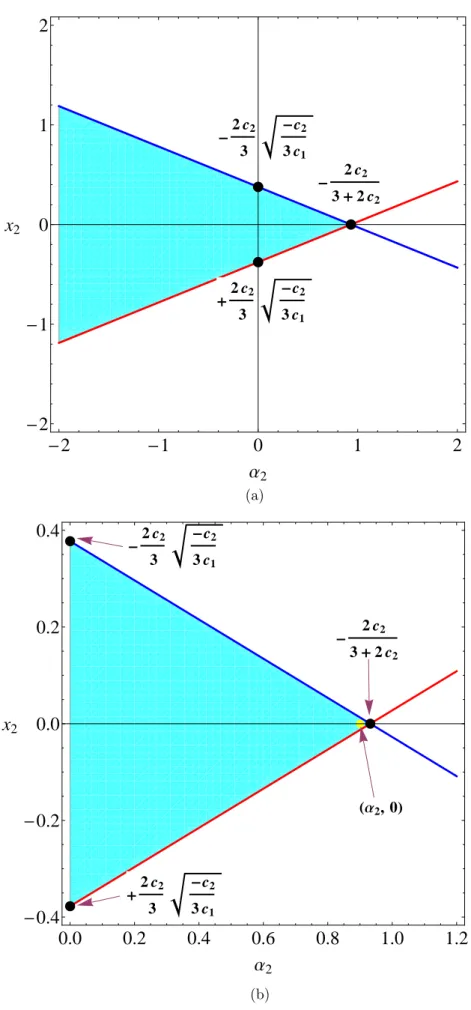
verified. Thus, the pseudo singular manifold is of saddle-type iff q < 0. But, as recalled previously, one coordinate is undetermined, say x2without
loss of generality. So, the eigenvalues (46) of the characteristic polynomial are also functions of the variable x2 and of the parameters of system (30).
Now, let suppose that one parameter, say without loss of generality α2(see
Sec. 6), modifies the nature of the pseudo singular manifold. Condition
C2, i.e. q < 0 is then represented in the space (x2, α2) by a straight line
defining a region within which the pseudo singular points are of saddle type. In other words, it means that by choosing a value of the coordinate
x2 inside this region ensures that the pseudo singular point would be of
4.7. Canard existence in R4
In a paper entitled “A propos de canards” Wechselberger [47] stated, while using a standard polynomial change of variables, that any n-dimensional singularly perturbed systems with k slow variables (k > 2) and m fast (m > 1) (1) can be transformed into the following “normal form” (see Appendix B): ˙ x1=˜ax2+ ˜by1+ O ( x1, x22, x2y1, y12 ) + εO (x1, x2, xk, y1) , ˙ x2=1 + O (x1, x2, y1, ε) , ˙ xj=˜cj+ O (x1, x2, y1, ε) , j = 3, . . . , k ε ˙y1=x1+ y21+ x1y1O (x2, . . . , xk) + y12O (x1, y1) + εO (x1, x2, y1, ε) (48)
which is a generalization of system (28). We will establish in Appendix B for any four-dimensional singularly perturbed systems (30) with k = 3
slow variables and m = 1 fast variable that
˜ a = 1 2f 2 2 ( ∂2g1 ∂x2 2 ∂2g1 ∂y2 1 − ( ∂2g1 ∂x2∂y1 )2 ) +1 2f2 ∂g1 ∂x1 ( ∂2g1 ∂y2 1 ∂f1 ∂x2− ∂2g1 ∂x2∂y1 ∂f1 ∂y1 ) +1 2f 2 3 ( ∂2g 1 ∂x2 3 ∂2g 1 ∂y2 1 − ( ∂2g1 ∂x3∂y1 )2 ) +1 2f3 ∂g1 ∂x1 ( ∂2g 1 ∂y2 1 ∂f1 ∂x3 − ∂2g1 ∂x3∂y1 ∂f1 ∂y1 ) + f2f3 ( ∂2g1 ∂x2∂x3 ∂2g1 ∂y2 1 − ∂2g1 ∂x2∂y1 ∂2g1 ∂x3∂y1 ) , ˜b =−∂g1 ∂x1 ∂f1 ∂y1 ,
Remark 3. Let’s notice that by posing f3= 0 in ˜a we find again a given
in Sec. 3.7.
Thus, in his article entitled “A propos de canards” Wechselberger [47, p. 3304] has provided in the framework of “standard analysis” a generalization of Benoˆıt’s theorem [6] (see Benoˆıt’s theorem above) for any n-dimensional singularly perturbed systems with k slow variables (k > 2) and m fast (m> 1). According to his Theorem 4.1(b) presented below he proved the existence of canard solutions for the original system (1).
Theorem 2.
In the folded saddle case of system (48) singular canards perturb to maxi-mal canards solutions for sufficiently smaxi-mall ε≪ 1.
As previously recalled, the method presented in this paper doesn’t use the “desingularized vector field” (37) but the “normalized slow dynamics” (36). So, we have the following proposition:
Proposition 2.
If the normalized slow dynamics (36) has a pseudo singular point of saddle type, i.e. if the sum σ2of all second-order diagonal minors of the Jacobian
matrix of the normalized slow dynamics (36) evaluated at a pseudo singular point is negative, i.e. if σ2< 0 then, according to Theorem 2, system (30)
exhibits a canard solution which evolves from the attractive part of the slow manifold towards its repelling part.
Proof.
By making some smooth changes of time and smooth changes of co-ordinates (see Appendix B) we brought the system (30) to the following “normal form”: ˙ x1= ˜ax2+ ˜by1+ O ( x1, ε, x22, x2y1, y12 ) , ˙ x2= 1 + O (x1, x2, y1, ε) , ˙ x3= 1 + O (x1, x2, y1, ε) , ε ˙y1= x1+ y12+ O ( εx1, εx2, εy1, ε2, x21y1, y31, x1x2y1 ) ,
Then, we deduce that the condition for the pseudo singular point to be of saddle type is ˜a < 0. According to Eqs. (46) it is easy to verify that
σ1= T r(J(F1,F2,F3,G1)) = λ1+ λ2=−˜b, σ2= 3 ∑ i=1 Jii (F1,F2,F3,G1) = λ1λ2= 2˜a.
So, the condition for which the pseudo singular point is of saddle type,
i.e. σ2< 0 is identical to that proposed by Wechselberger [47, p. 3298] in
his theorem, i.e. ˜a < 0.
So, Prop. 2 can be used to state the existence of canard solution for such systems. Application of Proposition 2 to the four-dimensional memristor canonical Chua’s circuits, presented in Sec. 6, will enable to prove the existence of generic “canards solutions” in such Memristor Based Chaotic Circuits.
5. THIRD-ORDER MEMRISTOR-BASED CANONICAL OSCILLATOR
Let’s consider the Memristor-Based canonical Chua’s circuit [27, 28] con-taining five circuits elements: two passive capacitors, one passive inductor, one negative resistor, and one active Chua’s flux controlled memristor (see Fig. 2).
FIG. 2. Memristor-Based canonical Chua’s circuit [28].
The parameter values used by Itoh and Chua [28, p. 1330001-14] i.e. are: C1= 1 10, C2= 1 0.47, G = L = 1, a =−2.0, b = 4.0.
5.1. Flux-linkage and charge phase space
Applying Kirchhoff’s circuit laws to the nodes A, B and the loop C of the circuit Fig. 2, Itoh and Chua [27, 28] obtained the following set of differential equations, i.e., the following memristor based chaotic circuit :
C1 dφ1 dt = q3− k (φ1) , C2 dφ2 dt =−q3+ Gφ2, Ldq3 dt = φ2− φ1. (49)
where the φ− q characteristic curve of the Chua’s memristor is given by the following piecewise-linear function:
q = k (φ) = bφ + a− b
By setting x = φ1, y = q3, z = φ2, ε = C1, β = 1 C2 , γ = G C2 and L = 1 the memristor based chaotic circuit (50) can be written:
dx dt = 1 ε[y− k (x)] , dy dt = z− x, dz dt =−βy + γz. (51)
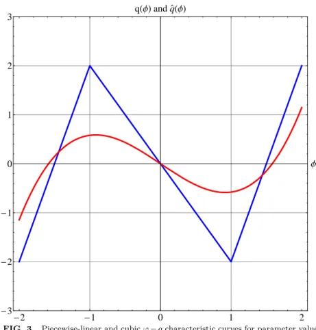
Following the works of Tsuneda [44], let’s replace the φ−q characteristic curve of the Chua’s memristor q(φ) which is given by the piecewise-linear function (51) by a smooth cubic nonlinear function ˆk(φ) = c1φ3+ c2φ for
which the parameters c1and c2are determined while using the least squares
method. The square error between k(φ) and ˆk(φ) is defined by:
S = ∫ d −d [ k(φ)− ˆk(φ) ]2 dφ (52)
where [−d, d] is an interval for approximation. Let’s note that in our case d is considered as a parameter such that|d| > 1. Solving ∂S/∂c1= 0
and ∂S/∂c2= 0, we find c1=− 35(a− b)(−1 + d2)2 16d7 , c2= (a− b)(21− 50d2+ 45d4) 16d5 + b. (53)
5.2. Piecewise-linear and cubic nonlinearity
While still using the same parameter values as Itoh and Chua [28, p. 1330001-14] i.e. C1= 1 10, C2= 1 0.47, G = L = 1, a =−2.0, b = 4.0,
the coefficients c1and c2have been chosen such that the extrema of both
piecewise-linear and cubic nonlinearity characteristic curves substantially coincides as exemplified on Fig. 3. This condition is realized for d = 3 and
c1=
280
729 ; c2=− 26 27.
-2 -1 0 1 2 -3 -2 -1 0 1 2 3 Φ qHΦL and q`HΦL
FIG. 3. Piecewise-linear and cubic φ− q characteristic curves for parameter values:
a =−2, b = 4 and d = 3.
So, let’s consider the memristor based chaotic circuit (51):
dx dt = 1 ε[y− k (x)] , dy dt = z− x, dz dt =−βy + γz, (54)
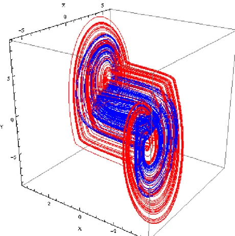
and let’s replace the piecewise-linear characteristic curves k(x) by the cubic ˆk(x) = c1x3+ c2x. First, let’s notice that both chaotic attractors
given respectively by Eqs. (51) & Eqs. (54) are quite similar as highlighted on Fig. 4.
FIG. 4. Memristor-Based canonical Chua’s circuits with piecewise linear (Eqs.
(51) in red) and cubic (Eqs. (55) in blue) functions for parameter values: ε = 1/10,
Now, let’s make the following variable changes in Eqs. (54) in order to apply the method presented in Sec. 3:
x→ z, y → −x, z → y. Thus, we have: dx dt = z− y, dy dt = βx + γy, dz dt = 1 ε[−x − k (z)] . (55)
This last transformation will enable to compare the condition (given be-low) for the existence of canard solutions in system (55) with those given in our previous works entitled “Canards from Chua’s circuits” [22].
Finally, let’s replace the variables (x, y, z) by (x1, x2, y1) and let’s apply
the method presented in Sec. 3 to the following system
dx1 dt = y1− x2, dx2 dt = βx1+ γx2, dy1 dt = 1 ε[−x1− k (y1)] . (56)
5.3. Critical manifold and constrained system
The critical manifold of this system (56) is given by −x1− k(y1) = 0.
According to Eq. (15) the constrained system on the critical manifold reads: ˙ x1= y1− x2, ˙ x2= βx1+ γx2, ˙ y1= y1− x2 − (c1y31+ c2y1) , 0 =−x1− ( c1y31+ c2y1 ) . (57)
5.4. Normalized slow dynamics
Then, by rescaling the time by setting t = −∂g1
∂y1
τ = (3c1y12+ c2) we
obtain the “normalized slow dynamics”:
˙ x1= (y1− x2) ( 3c1y12+ c2 ) = F1(x1, x2, y1) , ˙ x2= (βx1+ γx2) ( 3c1y12+ c2 ) = F2(x1, x2, y1) , ˙ y1= x2− y1= G1(x1, x2, y1) , 0 =−x1− ( c1y13+ c2y1 ) . (58)
5.5. Pseudo singular points
According to Eq. (18), the pseudo singular points of system (56) are:
˜ x1=± 2c2 3 √ −c2 3c1 , ˜x2=∓ √ −c2 3c1 , ˜y1=∓ √ −c2 3c1 . (59)
Let’s notice that these pseudo singular points are independent of the parameter γ. The Jacobian matrix of system (58) evaluated at the pseudo
singular points reads:
J(F1,F2,G1)= 0 0 0 0 0 −2γc2+ 4βc2 2 3 0 1 −1 (60)
Remark 4. Although, the pseudo singular points have not been shifted at the origin Benoˆıt’s generic hypotheses (20-21) are satisfied.
5.6. Canard existence in third-order memristor Chua’s circuit
According to Eqs. (25) we find that:
p = σ1= T r [J ] =−1,
q = σ2=
2
3c2(3γ− 2βc2) .
Thus, according to Prop. 1, the pseudo singular points are of saddle-type if and only if:
2
∆ = p2− 4q > 0 and q < 0.
So, we have the following conditions C1 and C2:
C1: ∆ = 1 + 4(−2c2)(γ− 2βc2 3 ) > 0, C2: q = 2c2(γ− 2βc2 3 ) < 0. (61)
Since the pseudo singular points are independent of the parameter γ let’s choose γ as the “canard parameter” or “duck parameter”. Obviously, it appears that if the condition C2 is verified then the condition C1 is de
facto satisfied14. Finally, the pseudo singular points are of saddle-type if
and only if we have:
γsaddle−node=
2βc2
3 < γ. (62)
where γsaddle−node represents the critical value of the parameter γ for
which one of the two remaining eigenvalues λ1 or λ2 of the
eigenpoyno-mial associated with the Jacobian matrix (60) vanishes. With this set of parameters ε = 1/10, β = 0.47, a = −2, b = 4, d = 3, c1 = 280/729,
c2=−26/27
γsaddle−node=
2βc2
3 ≈ −0.3.
5.7. Fixed points stability and Routh-Hurwitz’ theorem
However, as pointed out in our previous works entitled “Canards from Chua’s circuits” [22] the system (56) admits, except the origin, two fixed points, the stability of which could preclude the existence of “canards solu-tions”. So, let’s compute the fixed points of system (56) and analyze their stability. System (56) admits except the origin the following fixed points:
x∗1=± γ β √ γ− c2β c1β , x∗2= y1∗=∓ √ γ− c2β c1β . (63)
The eigenpolynomial equation of the Jacobian matrix of system (56) evaluated at these fixed points (63) reads:
14Keep in mind that c
2 is generally negative so that the characteristic curve admits
ελ3+ λ2(3γ
β − γε − 2c2) + λ(1−
3γ2
β + βε + 2γc2) + 2(γ− βc2) = 0 (64)
Let suppose that all the parameters are fixed except γ, i.e. the “duck parameter”. There are two methods to analyze the stability of fixed points as functions of the “duck parameter” value. The first is to solve the above third degree eigenpolynomial equation (64) with the Cardano’s method and the second consists in using the Routh-Hurwitz’ theorem [39, 25]. This latter method enables to easier analyze the stability of the fixed points as functions of a parameter. According to Routh-Hurwitz’ theorem, the
eigenpolynomial equation can be written as:
a3λ3+ a2λ2+ a1λ + a0= 0.
It states that if D1= a1 and D2 = a1a2− a0a3 are both positive then
eigenpolynomial equation would have eigenvalues with negative real parts.
In other words, if D1 and D2 are positive the fixed points will be stable.
In the case of the eigenpolynomial equation (64) we have:
D1=1− 3γ2 β + βε + 2γc2, D2=− 2ε (γ − βc2) + ( 3γ β − γε − 2c2 ) ( 1−3γ 2 β + βε + 2γc2 ) . (65) By setting: ε = 1/10, β = 0.47, a =−2, b = 4, d = 3, c1 = 280/729,
c2=−26/27 and while considering that the “duck parameter” γ can vary,
D1 and D2 are respectively polynomial equations of degree two and three
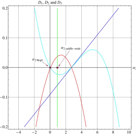
in γ. These quadratic and cubic functions D1and D2have been plotted on
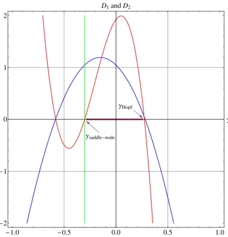
Fig. 5. One can see that between the lower limit called γsaddle−nodeand, the
upper limit called γHopf corresponding to the value of the parameter γ for
which the real parts of both complex eigenvalues vanishes (see proof in Ap-pendix C), D1and D2are strictly positive. So, for γ ∈ [γsaddle−node, γHopf]
(purple rectangle on Fig. 5) the fixed points are stable while for γ > γHopf
they are unstable. With this set of parameters,
Γsaddle-node ΓHopf -1.0 -0.5 0.0 0.5 1.0 -2 -1 0 1 2 Γ D1and D2
FIG. 5. Routh-Hurwitz determinants of system (56). D1in blue, D2in red and the
saddle-node axis γ = 2βc2/3 in green for parameter values: ε = 1/10, β = 0.47, a =−2,
Thus, it appears from what precedes and from Prop. 1 that “canards solutions” may be observed in system (56) for γDuck values such that:
γsaddle−node=
2βc2
3 < γHopf < γDuck (66)
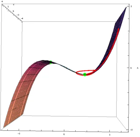
On Fig. 6, numerical “canards solutions” and slow manifold of system (56) have been plotted for the “duck parameter” γDuck= 0.3275 (all other
parameters are the same as indicated above). Due to the symmetry of the system (56), any of the two pseudo singular points plotted in green on Fig. 6 was chosen as initial condition.
FIG. 6. Numerical “canards solutions” and slow manifold of system (56) for param-eter values: ε = 1/10, β = 0.47, γDuck= 0.3275, a =−2, b = 4, d = 3, c1= 280/729
5.8. Particular case
In a previous work entitled “Canards from Chua’s circuits”, Ginoux et al. [22] have studied the system (56) with the following particular parameters:
γ = β = α c1=
1
3 c2=−1
First, let’s replace these parameters in the above conditions C1 and C2
(61). We have: C1: ∆ = 1 + 40α 3 > 0, C2: q =− 10α 3 < 0.
Obviously, if α > 0, then both conditions C1 and C2 are verified. This
is exactly the result provided by Itoh and Chua [26] as it has been noticed in Ginoux et al. [22, p. 1330010-4]. However, it has been also remarked in our same previous paper [22] that the system (56) admits, except the origin, two fixed points, the stability of which could preclude the existence of “canards solutions”. By setting: γ = β = α, c1 = 13 and c2 =−1 in
Eq. (63) we find again the fixed points obtained by Ginoux et al. [22, p. 1330010-4]:
x∗1=±√6, x∗2=∓√6, y∗1=∓√6.
Moreover, still using the Routh-Hurwitz’ theorem and by setting: γ =
β = α, c1= 13 and c2=−1 in Eq. (65) we find that:
D1= 1− 5α + εα,
D2= α2
(
5ε− ε2)− 25α + 5.
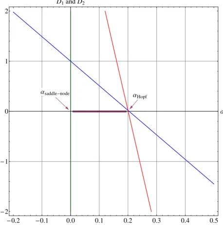
Functions D1 and D2 have been plotted on Fig. 7 on which one can
see that between the lower limit called αsaddle−node and, the upper limit
called αHopf corresponding to the value of the parameter α for which the
real parts of both complex eigenvalues vanishes, D1 and D2 are strictly
positive. So, for α∈ [αsaddle−node, αHopf] (purple rectangle on Fig. 7) the
fixed points are stable while for α > αHopf, i.e. α > 1/5 they are unstable.
Thus, it appears from what precedes and from Prop. 3 that “canards solutions” may be observed in system (56) provided that:
ΑHopf Αsaddle-node -0.2 -0.1 0.0 0.1 0.2 0.3 0.4 0.5 -2 -1 0 1 2 Α D1and D2
FIG. 7. Routh-Hurwitz determinants of system (56). D1 in blue, D2 in red and
the the saddle-node axis γ = 0 in green for parameter values: ε = 1/10, β = γ = α,
![FIG. 1. “Canard cycle” of the Van der Pol equation, Diener [13, p. 45].](https://thumb-eu.123doks.com/thumbv2/123doknet/14623558.733989/3.892.258.615.474.672/fig-canard-cycle-van-der-pol-equation-diener.webp)
![FIG. 2. Memristor-Based canonical Chua’s circuit [28].](https://thumb-eu.123doks.com/thumbv2/123doknet/14623558.733989/27.892.280.634.292.458/fig-memristor-based-canonical-chua-s-circuit.webp)
![FIG. 8. Memristor canonical Chua’s circuit [18].](https://thumb-eu.123doks.com/thumbv2/123doknet/14623558.733989/39.892.284.634.393.515/fig-memristor-canonical-chua-s-circuit.webp)