UNIVERSITÉ DU QUÉBEC
THÈSE PRÉSENTÉE À
L'UNIVERSITÉ DU QUÉBEC À TROIS-RIVIÈRES
COMME EXIGENCE PARTIELLE DU DOCTORAT EN GÉNIE ÉLECTRIQUE
PAR SIMON HIS SEM
CONTRIBUTION À LA CONCEPTION DE CONTRÔLEUR POUR DES SYSTÈMES DE TYPE BOÎTES NOIRES ET DES SYSTÈMES À HAUT DEGRÉ DE FONCTIONS
DE TRANSFERT
Université du Québec à Trois-Rivières
Service de la bibliothèque
Avertissement
L’auteur de ce mémoire ou de cette thèse a autorisé l’Université du Québec
à Trois-Rivières à diffuser, à des fins non lucratives, une copie de son
mémoire ou de sa thèse.
Cette diffusion n’entraîne pas une renonciation de la part de l’auteur à ses
droits de propriété intellectuelle, incluant le droit d’auteur, sur ce mémoire
ou cette thèse. Notamment, la reproduction ou la publication de la totalité
ou d’une partie importante de ce mémoire ou de cette thèse requiert son
autorisation.
UNIVERSITÉ DU QUÉBEC
THESIS PRESENTED TO
UNIVERSITÉ DU QUÉBEC À TROIS-RIVIÈRES
IN PARTIAL FULFILMENT OF THE REQUIEREMNTS OF THE DEGREE OF DOCTOR OF PHILOSOPHY
IN ELECTRICAL ENGINEERING
BY
SIMON HIS SEM
CONTRIBUTION TO THE DESIGN OF CONTROLLER FOR SYSTEMS OF BLACK BOXES TYPE AND SYSTEMS WITH HIGH DEGREE OF TRANS FER FUNCTIONS
UNIVERSITÉ DU QUÉBEC
À
TROIS-RIVIÈRESDOCTORAT EN GÉNIE ÉLECTRIQUE (PH.D.)
Programme offert par l'Université du Québec à Trois-Rivières
CONTRIBUTION À LA CONCEPTION DE CONTRÔLEUR POUR DES SYSTÈMES DE TYPE BOÎTES NOIRES ET DES SYSTÈMES À HAUT DEGRÉ DE FONCTIONS
DE TRANSFERT
PAR SIMON HIS SEM
Prof. Mamadou L. Doumbia, directeur de recherche Université du Québec à Trois-Rivières
Prof. Alain Goupil, président du jury Université du Québec à Trois-Rivières
Prof. Pelope Adzakpa, évaluateur Cegep de la Gaspésie et des Iles
Prof. Hicham Chaoui, évaluateur Université Carleton à Ottawa
Abstract
This research presents new reduction method for black box systems and systems with high order transfer functions. This new technique is essentially based on the nature of the three most common output responses with no overshoot, with overshoot only or with overshoot and oscillations. The approach is based on the concept oftwo similar systems that are not identical. This similarity is made on significant weighted elements that characterize the black box system. The controller will be designed based on the simple projected similar system and applied to the black box or higher order systems. The characteristic of this new reduction method is that every system can be reduced to a similar first order system with the same identified significant weighted elements that will be clearly defined. The merit of this new reduction technique is to avoid ail mathematical equations to model the complex system and also to avoid huge mathematical equations to reduce its transfer function to an identical reduced system. The performance of the new reduction method was evaluated and compared with sorne reduction methods taken from the literature.
New systems caIled Fibonacci systems are introduced. They are derived from an original first order transfer function. Their characteristics and behaviors are quite impressive and their output signaIs present multiple intermediate steady states which make them irreducible to a lower order specifically second or third order. The application of reduction methods to these systems in the literature will not be possible. Their polynomial coefficients follow specific distribution with respect to the Golden ratio. The pole locations of these transfer functions follow the Fibonacci pattern and they can be created to an infinite degree following a simple recursive process. These functions have multiple resonance and anti-resonance frequencies organized in a perfect way with respect to each other. Each Fibonacci system has two weIl
defined Fibonacci boundary systems using Pascal' s triangle. The behavior of these systems could describe coupled systems applications, transmission lines, impedance matching and other applications that can be modelled by an infinite LC ladders or infinite spring mass chain.
Keywords: High order transfer function, reduction method, black box system, Pade approximation, Integral square error (ISE), similar systems, Fibonacci irreducible systems, infinite LC ladder and infinite spring mass chain.
Avant-propos
Au terme de ce travail, je tiens à témoigner ma profonde reconnaissance à mon directeur de
recherche, le professeur Mamadou Lamine Doumbia pour le rôle prépondérant qu'il ajoué
dans ma motivation et ma formation scientifique. L'ampleur de ses connaissances et la qualité de ses conseils m'ont permis de réaliser ce projet. Je le remercie pour la confiance qu'il a témoignée à mon égard.
Au cours de ce travail de recherche j'ai eu à apprécier le soutien moral de tous mes amis qui ont contribué de près ou de loin à l'achèvement de ce travail.
Mes remerciements vont enfin à tous les membres de ma famille et tout spécialement à ma femme et ma fille qui m'ont aidé moralement. Sans elles, je n'aurais pas été en mesure de contribuer à la recherche scientifique. J'ai une pensée très spéciale pour mes parents, que leurs âmes reposent en paix; eux qui m'ont inculqué le sens du sérieux, le respect et le travail bien fait.
Table of Contents
Abstract ... iv Avant-propos ... vi
Chapter 1: Introduction ... 1
1.1 Brief history on reduction methods ... 1
1.1.1 Integral square error method ... 1
1.1.2 Pade approximation method ... 1
1.1.3 Other reduction methods ... 2
1.2 Research goals ... 2
1.2.1 Main objective .................... 2
1.2.2 Contribution ofthis thesis .............. 2
1.2.3 Thesis structure ... 3
1.2.4 Publications .... 4
Chapter 2: Classical reduction methods ... 5
2.1 Introduction ... 5
2.2 Integral square error reduction method ... 5
2.2.1 The case of an impulse input ... 6
2.2.2 The case of a constant input. ... 9
2.2.3 Controller design based on ISE method ... 10
2.2.4 Analysis of the ISE and its controller design ... Il 2.3 Pade approximation method ... 12
2.3.2 Analysis of pade and its controller design ... 15
2.4 Conclusion ... 16
Chapter 3: New proposed reduction method ... 17
3.1 Similar systems new approach theory ... 17
3.2 Similar systems application to black box ... 18
3.3 Application to different black box systems output ... 22
A. Case study 1 ... 22
B. Case study 2 ... 24
C. Case study 3 ... 26
D. Case study 4 ... 27
E. Case study 5 ... 29
3.4 PI Controller design for black box systems ... 31
3.5 Controller design approach based on similar system ... 33
A. Case study 1 ... 33
B. Case study 2 ... 34
C. Case study 3 ... 35
D. Case study 4 ... 36
E. Case study 5 ... 37
3.6 New approach and classical reduction method comparison ... 38
3.7 Conclusion ... 42
4.2 Fibonacci systems with irreducible transfer functions ... 43
4.3 Fibonacci systems characteristics ... 45
4.4 Fibonacci systems analysis ... 50
4.5 Fibonacci boundary systems ... 53
4.6 Case studies and simulations ... 55
4.7 Controller Design New Approach applied to Fibonacci systems ... 62
4.8 Controller Design New Approach limitation ... 64
4.9 Conclusion ... 66
Chapter 5: Fibonacci wave functions application to LC ladder network ... 67
5.1 Introduction ... 67
5.2 RC Fibonacci electrical circuit (RC-FEC) ... 67
5.3 RC-FEC and FWFs simulation (RL-FEC) ... 71
5.4 RL Fibonacci electrical circuit. ... 75
5.5 Simulation ofFWF and its corresponding RL-FEC ... 78
5.6 Nth Order LC Ladder RC-FEC and RL-FEC general model ... 81
5.7 Fibonacci wave functions applied to transmission lines ... 89
5.8 Conclusion ... 93
Chapter 6: Fibonacci wave functions application to spring mass chain ... 95
6.1 Introduction ... 95
6.2 Fibonacci Spring mass chain ... 95
6.3 Simulation ofFMSC ... 101
6.5 FSMC with infinite and zero kv viscous damper. ... 112
6.6 Conclusion ... 115
Chapter 7: Fibonacci wave functions application to inverse LC ladder network ... 117
7.1 Introduction ... 117
7.2 Inverse RC Fibonacci electrical circuit (iRC-FEC) ... 117
7.3 Simulation ofiRC-FEC AND iFWFs ... 121
7.4 Inverse RL Fibonacci electrical circuit (iRL-FEC) ... 125
7.5 Simulation of iRL-FEC and iFWFs ... 129
7.6 Nth order inverse LC ladder iRC-FEC and iRL-FEC general model ...... 131
7.8 Controller Design new Approach applied to iFWFs ... 141
7.9 Inverse Fibonacci boundary wave functions ... 143
7.10 Conclusion ... 149
Chapter 8: General conclusion ... 150
8.1 General conclusion ... 150
References ... 154
Appendix A: Résumé étendu ... 160
A.l Introduction ... 160
A.l.l Problématique de recherche ................... 160
A.l.2 Objectifde recherche ... 161
A.l.2.l Contribution de recherche ... 161
A. 2.1 Intégral de l'erreur quadratique (ISE) ... 163
A. 2. 2 Approximation pade ... 164
A.2.3 Autres méthodes de réductions ...... 165
A.3 Nouvelle approche de réduction ... 165
A. 3.1 Application de l'approche des systèmes similaires aux boites noires ... 167
A.4 Systèmes irréductibles et limitations des méthodes classiques ... 168
A.5 Étude de cas et simulations ... 171
A.6 Nouvelle approche de conception de contrôleur appliquée aux systèmes de Fibonacci ... 172
A.7 Systèmes de Fibonacci appliqués aux Systèmes électriques et mécaniques ... 175
A.7.1 Réseau récurrent LC de Fibonacci ... 175
A.7.2 Chaine de masse-ressort de Fibonacci ... 177
A.7.3 Réseau récursif inverse LC de Fibonacci ...... 179
LIST OF FIGURES
Figure 2.1: Open loop GfE(S), G~SE(S) and GfD(S) ... 10
Figure 2.2: Closed loop GJSE (s), G~SE (s) and GfD (s) ..... Il Figure 2.3: Open loop Gtade(s) and Gtade(s) ............... 14
Figure 2.4: Closed loop Gtade(s) and Gfade(s) ...... 15
Figure 3. 1: a) Two identical sets b) Two similar sets ... 17
Figure 3.2: Two similar systems A and B ... 18
Figure 3. 3: Real system with access to its inputs values and its outputs responses ... 18
Figure 3.4: Output response for real system with no overshoot ... 19
Figure 3.5: Output response for real system with overshoot and oscillations ... 19
Figure 3. 6: Output response for real system with overshoot and no oscillation ... 19
Figure 3.7: Output response of the real system in open-Ioop ... 22
Figure 3. 8: Output response of the real and reduced open-Ioop system ... 24
Figure 3.9: Output response of the real open loop system with no overshoot. ... 24
Figure 3. 10: Real and reduced system output response in open-Ioop ... 25
Figure 3. Il: Output response of the real system with no overshoot with oscillations ... 26
Figure 3. 12: Output of the real and reduced system response in open loop ... 27
Figure 3. 13: Output of the real system in open loop with overshoot and oscillations ... 28
Figure 3. 14: Output response of the three systems-Real, reduced in [4] and proposed similar system ... 29
Figure 3. 15: Output of the real system in open loop with overshoot only ... 30
Figure 3. 16: Output response of the real, reduced system in [3] and proposed similar system ... 31
Figure 3. 17: Similar closed-Ioop system ... 31
Figure 3.18: Real and reduced c\osed loop with disturbance. (Ç = 0.99 and Wn = 1.48 radis) ... 33
Figure 3.20: Real and reduced closed loop with disturbance. (Ç = 0.99 and Wn = 0.45 radIs) ... 34
Figure 3. 21: Real and reduced c\osed loop with disturbance. (Ç = 0.99 and Wn = 2.55 radIs) ... 35
Figure 3. 22: Real and reduced c\osed loop with disturbance.
ç
= 0.7 and Wn = 3.57 rad/s ... 35Figure 3.23: Real and reduced closed loop with disturbance. (Ç=1.5; wn=1.28rad/s) ... 36
Figure 3. 24: Real and reduced c\osed loop with disturbance. Ç=2; wn=300rad/s ... 36
Figure 3. 25: Real and reduced c\osed loop with disturbance. (Ç=0.99 wn=100rad/s) ... 37
Figure 3. 26: Real and reduced c\osed loop with disturbance. (Ç=2; wn=100rad/s) ... 38
Figure 3.27: Real and similar systems output response ... 39
Figure 3.28: Real and reduced c\osed loop Ç=1.5; wn=1.33rad/s ... 40
Figure 3. 29: Real and similar systems output response ... 41
Figure 3. 30: Real and reduced c\osed loop for Ç=I.5; wn=2.66rad/s ... 41
Figure 4. 1: FWFs recursive process ... 44
Figure 4.2: Real part of gi~·l)(S) poles for case #1.. ... 50
Figure 4.3: Real part of gi~,4)(s) poles for case #2 ... 50
Figure 4.4: Imaginary part of gi~·l)(S) poles for case #1.. ... 51
Figure 4.5: Imaginary part of gi~,4)(s) poles for case #2 ... 51
Figure 4. 6: Case # 1- Odd coefficients (black). Even coefficients (Hashed) of deni~l) (s) ... 52
Figure 4.7: Case #2-Odd coefficients (black). Even coefficients (Hashed) of deni~4) (s) ... 52
Figure 4.8: FWF g~1.0)(S) (n = 37,38,39 and 40) outputs with unit input. ... 54
Figure 4.9: FWF g~1.0) (s) (n
=
37,38,39 and 40) outputs with input pulse of 30s . ... 54Figure 4.10: Bode plots ofFWFs g?l)(S), , ... gi~·l)(S) ... 56
Figure 4.12: Poles and zeros of 9i1,1)(S), ... 9~~1)(S) ... 57
Figure 4.13: Output response ofodd FWFs 9i1,1) (s), 9g,1)(S) ... 57
Figure 4. 14: Output response of odd FWFs 9i~,1) (s), 9j~,1) (s) .................. 58
F· Igure4 . ·15 0 : utput response 0 0 f dd FWF s 91 (1,1)() S ,911 (1,1)() s, 921 (1,1)() (1,1)() (1,1)() S, 931 S, 939 S ... . 58
Figure 4.16: Output response ofeven FWFs 9~1,1)(s), 9g,1)(S) ... 58
Figure 4. 17: Output response of ev en FWFs 9~1,1) (s), 9~~,1) (s) ..... 59
· (1,1) (1,1) (1,1) (1,1) (1,1) FIgure 4. 18:0utputresponseofevenFWFs92 (s), 912 (s), 922 (s), 932 (s), 940 (s) .. 59
Figure 4. 19: Output response of odd and even FWFs (1,1) () (1,1) () (1,1) () (1,1) () (1,1) () (1,1) () (1,1) () (1,1) () (1,1) () (1,1) ( ) 91 S , 911 s , 921 s, 931 s, 939 s, 92 S ,912 S, 922 S, 932 S, 940 S ... 59
Figure 4.20: Bode plots ofFWFs 9i1,4) (s), , ... 9~~4)(S) . ... 60
· (1,4) (1,4) (1,4) FIgure 4. 21: BodepiotsofFWFs91 (s), 939 (s), 940 (s) ... 60
· (1,4) (1,4) FIgure 4.22: Poles and zeros ofFWFs 91 (s), ... 940 (s) ... 61
· (1,4) (1,4) (1,4) (1,4) (1,4) FIgure 4.23: Output response ofFWFs gl (5), gl1 (s), g21 (5), g31 (S),g39 (5) ... 61
· (1,4) (1,4) (1,4) (1,4) (1,4) Flgure4.24:0utputresponseofFWFs92 (S),912 (S),922 (S),932 (S),940 (s) .... 61 · (1,4) (1,4) (1,4) (1,4) (1,4) Flgure4.25:0utputresponseofFWFs91 (S),911 (S), 921 (S),931 (S),939 (s), (1,4) (1,4) (1,4) (1,4) (1,4) 92 (s), 912 (S), 922 (S),932 (S),940 (s) . ...... 62
Figure 4.26: Output response in closed loop ofFWFs (1,1) (1,1) (1,4) (1,4) 91 (s), .... ·91 (S), 91 (s), ... 940 (s) . ...... 64
· (1,0) (1,0) (1,0) (1,0) (1,0) FIgure 4. 27: Outputresponse ofFWFs 92 (S),912 (S), 922 (S),932 (S),940 (s) ... 64
· (1,0) (1,0) (1,0) (1,0) FIgure 4. 28: OutputresponseofFWFs, 911 (S), 921 (S),931 (S),939 (s) ... 65
· . (1,0) (1,0) FIgure 4.29: Output response In closed loop ofFWFs 9 1 (s), ... 940 (s) . ... 65
Figure 5. 1: First order RC-FEC ... 68
Figure 5. 2: Second order RC-FEC ... 68
Figure 5. 3: Third order RC-FEC ... 69
Figure 5. 4: nth even order RC-FEC ... 70
Figure 5.5: nth odd order RC-FEC ... 70
Figure 5. 6: FWF RC-FEC
(:)ici
1)=
C*
g~~,l) (s) & Matlab-Simulink model with li=
1 V ... 731 Figure 5. 7: FWF RC-FEC (O)~~l)
=
L*
gg,l)(S) & Matlab-Simulink model with li=
lA ... 74Figure 5. 8: First order RL-FEC ... 75
Figure 5.9: Second order RL-FEC ... 75
Figure 5. 10: First order RL-FEC ... 76
Figure 5. Il: nth even order RL-FEC ... 77
Figure 5. 12: nth odd order RL-FEC ... 77
Figure 5.13: FWF RL-FEC
(O)ici
1)=
Lg~~,l)(S) & Matlab-Simulink model with li=
lA ... 79Figure 5.14: FWF RL-FEC (:)~~1) = Cg~~,l)(S) & Matlab-Simulink model with Vi = lV ... 80
1 . V (11) ( 1 1 ) . 1 (11) FIgure 5. 15: RL-FEC and RC-FEC order 40; ((1')40
=
L940' (s), IL=
lA)) (((;)40=
C*
1 g~~,l)(S), Vi=
lV)) ... 81Figure 5. 16: nth even order RC-FEC. ... 82
Figure 5. 17: nth even order RC-FEC Model using FWFs for each CUITent and voltage branch .... 82
Figure 5. 18: nth even order RC-FEC Model using FWFs for each flux and charge branch ... 82
Figure 5. 19: nth even order RL-FEC ... 83
Figure 5. 20: nth even order RL-FEC Model using FWFs for each CUITent and voltage branch ... 83
Figure 5. 21: nth even order RL-FEC Model using FWFs for each flux and charge branch ... 83
Figure 5. 22: Matlab-Simulink RC-FEC circuit and proposed FWF general model for 1~~,4) with input Vi = lV ... 84
Figure 5. 23: Matlab-Simulink RC-FEC circuit and proposed FWF general model for V3~1,4)with
input Vi
=
IV ...... 84Figure 5. 24: Matlab-Simulink RC-FEC and FWF general model (~(1,4), ~(1,4), .. , V3~1,4)) ... 85
Figure 5. 25: Matlab-Simulink RC-FEC and FWF general model (l~l,4), I~l,4), .. , I~~,4)) ...... 85
Figure 5. 26: Matlab-Simulink RC-FEC and FWF general model
(l~~,l),
Vi = IV, R =Jf) ...
86Figure 5. 27: Matlab-Simulink RC-FEC and FWF general model
(~~1,1),
Vi=
1 V, R=
Jf)
...
87Figure 5. 28: Matlab-Simulink RC-FEC and FWF general model
(~(1,1),
V3(1,1), .. , VS,l), R =Jf)
... 87Figure 5. 29: Matlab-Simulink RC-FEC and FWF general model (ly,l), /2,1), .. ,
I~~,l)
,
R =Jf).
88 Figure 5.30: nth even order RC-FEC general model using energy wave between branches ... 88Figure 5. 31: Matlab-Simulink RL-FEC and FWF general model (V4~1,O), Ii
=
lA, R=
On) ... 92Figure 5. 32: Matlab-Simulink RL-FEC and FWF general model (l~~'O), Ii
=
lA, R=
On) ... 92Figure 5.33: Matlab-Simulink RC-FEC and FWF general model (~~l,O), Vi = IV 35s pulse, R
=
000) ....... 92Figure 5. 34: Matlab-Simulink RC-FEC and FWF general model (l~~'O), Vi
= 1
V 35s pulse, R=
oon) ................. 93Figure 6. 1: First order of FSMC ... 96
Figure 6.2: Second order ofFSMC ... 96
Figure 6.3: Third order ofFSMC ... 97
Figure 6. 5: Fifth order of FSMC ... 98
Figure 6. 6: nth even order ofFSMC ...... 98
Figure 6. 7: nth odd order of FSMC ... 99
F" Igure . 6 8' . FMSC (F(k40 ,Xm)) -- m
*
940 (k,xm )() s , v[ -. - 1 / ) m s ............ 103F' Igure . . 6 9' FSMC ( V(k,xm ) - ~
*
(k,xm )() F· - lN) 39 - ks 939 s, [- ... 104Figure 6. 10: nth even order FSMC Model using FWFs for each section for (v?,Xm), Fj(k,Xm)) variables ... 105
Figure 6. Il: nth ev en order FSMC Model using FWFs for each section for (I1Y'Xm), x?'Xm)) .. 105
Figure 6.12: FSMC general model for F4~,4) with input Vi
= Im/s) ..
... 106Figure 6. 13: FSMC general model for v~~,4)with input Vi
= Im/s)
... 106Figure 6. 14: FSMC general model for (FP,4), F4(1,4), .. , F4~,4). with Vi
= Im/s) ...
... 107' . (1,4) (1,4) (1,4) _ FIgure 6.15. FSMC general model for (v1 ,v4 " " V39 .for Vi - Im/s) ... 108
Figure 6. 16: FSMC general model for F4~,1) with input Vi = 1, kv = .Jmks ) ... 109
Figure 6. 17: FSMC general model for vJl,1)with input Vi
=
1, kv=
.Jmks) ... 109Figure 6. 18: FSMC general model for F}l,1), F4(1,1) .. , F4~,1), kv
=
.Jmks) ... 110Figure 6. 19: FSMC general model (V;l,l), vy,l), .. , V~!,l), kv
=
.Jmks) ... 111Figure 6. 20: nth ev en F-Spring-Mass Model using FWFs for energy transfer between sections. 112 ' . (1,0) _ _ FIgure 6.21. FSMC general model (F40 ,vi - lm/s, kv - 0) ... 114
Figure 6.22: FSMC general model (F4~'0), Vi
= Im/s
(pulse of 20s),kv= 0) ... 114
Figure 6. 23: FSMC general model (vy,O\ Vi
= lm/s,
kv= 0 ) ... 114
Figure 7. 1: First order iRC-FEC ... 118
Figure 7. 2: Second order iRC-FEC. ... 118
Figure 7. 3: Third order iRC-FEC ... 119
Figure 7. 4: nth even order iRC-FEC ... 119
Figure 7.5: nth odd order iRC-FEC ... 120
Figure 7.6: iRC-FEC ((0)~14~
,
=
~*
9~~~) (s) with li=
lA) ... 124Figure 7. 7: RC-FEC ((:)
,
~13~)=
~*
9~13!)(S) with Vi=
lV ...... 125Figure 7. 8: First order iRL-FEC ... 125
Figure 7. 9: Second order iRL-FEC ... 126
Figure 7. 10: Third order iRL-FEC ... 126
Figure 7. Il: nth even order iRL-FEC ... 127
Figure 7. 12: nth odd arder iRL-FEC ... 128
Figure 7. 13: iRL-FEC
((:)~14~)
,
=
~
*
9~~~)(S)
, Vi=
lV ......................... 129F· Igure7 14·'RL FEC . .1 - ((V
1;
O)(l,l) -39 --C
1*
9-39 S (1,1) ( ) . wlt h 1 - lA) i - ....... 130Figure 7. 15: iRL-FEC and iRC-FEC order 40 . ((~)(1,1)
=
~*
9(l,l)(S) Vi=
lV))((°/
1,1)=
, Vi -40 L - 4 0 ' Ii -39 ~*
9~j!)(s), li=
lA)) ......... ...... 131Figure 7. 16: nth even order iRC-FEC ... 132
Figure 7. 17: nth even order iRC-FEC Madel using iFWFs for each CUITent and voltage branch. 132 Figure 7. 18: nth even arder iRL-FEC ... 132
Figure 7. 19: nth ev en order iRL-FEC Model using IFWFs for each CUITent and voltage branch.133 Figure 7. 20: iRC-FEC circuit and general model for V_(~o4)with input li
=
lA ... 134Figure 7.22: iRe-FEe circuit and general model for l~i:) with input li
=
lA ... 134Figure 7. 23: iRe-FEe circuit and general model for
v
S:/)
as integral of 1~94) with input li=
lA... 135 Figure 7. 24: Matlab-Simulink iRe-FEe and general model (V_(~,4), V_(~,4), . . , V_(~04)) across
inductors ... 135
Figure 7.25: Matlab-Simulink iRe-FEe and general model
(l~~,4), l~i4), .. ,l~i:)) across capacitors ... 136
Figure 7.26: Matlab-Simulink iRe-FEe and general model
(V_~lÔl),
li = lA, R =.fi)
...
137Figure 7.27: Matlab-Simulink iRe-FEe and general model
(l~~~),
li = lA, R =$)
as integral of V40(l,l) ... 137Figure 7.28: Matlab-Simulink iRe-FEe and general model
(l~i~),
li = lA, R =$) ...
138Figure 7.29: Matlab-Simulink iRe-FEe and general model
(V_(~91),
li=
lA, R=
$)
as integral of(1,1)
1-39 ... 138
Figure 7. 30: Matlab-Simulink iRe-FEe and general model
(V_(~Ol),
li=
lA, R=
$)
...
...
139Figure 7. 31: Matlab-Simulink iRe-FEe and general model
(l~i~),
li = lA, R =$ )
as integral of(1,1)
V-3D ...•..••....•...••...•... 140
Figure 7.32: Matlab-Simulin iRe-FEe and general model (VS,l),
V_(~,l),
.. ,V_(~Ol),
R =$)
acrossinductors ... 140
Figure 7.33: Matlab-Simulink iRe-FEe and general model
(l~il),
l~il),
..,l~i~),
R=
$)
across capacitors ... 141Figure 7. 34: Output response in closed loop ofFWFs
9~1/)(S), ... 9~~~)(S), 9~lt)(S), ... 9~~6)(s) ................ 143
Figure 7. 35: iRL-FEC and general model
(V_
(i3
0), Vi=
1 V, R=
oon) ... 146Figure 7.36: iRL-FEC and general model (I~~~), Vi
=
IV, R=
oon) as integralofv!i3
0) .......... 147Figure 7. 37: iRL-FEC and general model (I~~~), Vi
=
IV, R=
oon ) ... 147Figure 7.38: iRL-FEC and general model
(v!iz
O), Vi=
IV, R=
oon) as integral of l~~~) ... 147Figure 7. 39: iRC-FEC and general model (V_(!ÜO), li = lA ,R = On) ... 148
Figure 7. 40: iRC-FEC and general model (I~~~), li
=
lA ,R=
On) as integral of V!!ÜO) ••••••••••• 148 Figure 7. 41: iRC-FEC and general model (I~~~), li=
lA ,R=
0 n) ... 148Figure 7. 42: iRC-FEC and general model
(V_(ig
O), li=
lA, R=
0 n) as integral of l~~~) ... 149Figure A. 1: a) Ensembles identiques b) Ensembles similaires ... 165
Figure A. 2: Deux systèmes similaires A et B ... 166
Figure A. 3: Réponse de sortie du système réel sans dépassement... ... 167
Figure A. 4: Réponse de sortie du système réel avec dépassement et oscillations ... 167
Figure A. 5: Réponse de sortie du système réel avec dépassement et sans oscillations ... 168
Figure A. 6: FWFs processus récursif ... 169
Figure A. 7: Réponses de sortie en boucle ouverte des FWFs 9~1,1)(S), 9~~,1)(S), 9~~,1)(S), (1,1) (1,1) (1,1) (1,1) (1,1) (1,1) (1,1) 931 (S),939 (s), 92 (S), 9 12 (S), 922 (S), 932 (S), 940 (S) ............................ 171
Figure A. 8: Réponses de sortie en boucle ouverte des FWFs g~l,4)(S). (1,4) (1,4) (1,4) ,g22 (S),g32 (S),g40 (5) ... 172 Figure A. 9: Réponses de sortie en boucle ouverte des FWFs 9~1,4)(S), 9~~,4)(S), 9~~,4\S),
(1,4) (1,4) (1,4) (1,4) (1,4) (1,4) (1,4)
Figure A. 10: Réponses de sortie en boucle fermée des FWFs g?,l)CS), .. ,gi~,l)CS), g~l,4)CS),
(1,4)
.. , 9 40 CS) ... 174 Figure A. Il: nieme ordre pair RC-FEC ... 175
Figure A. 12: nieme ordre impair RC-FEC ... 176 FigureA. 13: nieme ordre pair de FSMC. ... 177 Figure A. 14: nieme ordre impair de FSMC ... 178 Figure A. 15: nieme ordre pair de iRC-FEC ... 179 Figure A. 16: niemeordre impair de iRC-FEC ... 180
LIST OF TABLES
Table 4. 1: Fibonacci transfer functions FWFs ... 44 Table 4.2: Fibonacci transfer functions for K, x = (1,1) ... 45 Table 4.3: Pascal's triangle rearrangement coefficients of ail den~1,1)(s) of Fibonacci transfer functions ... 46 Table 4.4: Denominator coefficients of FWFs with (K, x). [red numbers are for the case (K, x)
=
(1,1)] ... 47 Table 4.5: Pascal's triangle for Fibonacci transfer functions for ail den~k,X)(s) ......... 48 Table 4. 6: Pascal's triangle for Fibonacci boundary systems ... 53
Table 5.1: RC-FEC Fibonacci wave functions ... 71 Table 5. 2: Pascal's triangle general forrn with multiplication coefficients (K, xc) . ... 72 Table 5. 3: RL-FEC Fibonacci wave functions ... 78
Table 6. 1: F-Spring-Mass Chain Fibonacci wave functions FWFs ... 99 Table 6. 2: Pascal's triangle general form with coefficients of multiplication (k , xm ) . ..... 100 Table 6.3: Pascal's triangle for Fibonacci FMSC boundary systems (k , 0) & (k , (0) ... 113
Table 7. 1: iRC-FEC Fibonacci wave functions ... 120 Table 7.2: Pascal's triangle general form with multiplication coefficients (K, xc) ... 122 Table 7.3: Pascal's triangle general form Inverse with multiplication coefficients (K, xc) . ...... 123 Table 7. 4: iRL-FEC Fibonacci wave functions ... 128 Table 7.5: Pascal's triangle general forrn Inverse for boundary iFWF with (k, 0) & (k , (0) ... 146
Table A. 1: Les coefficients des dénominateurs des FWFs avec (K,x) .......................... 169
Table A. 2: Triangle de Pascal pour les den~k,X) des fonctions de transfert de Fibonacci ... 170 Table A. 3: Fonctions d'onde de Fibonacci RC-FEC ... 176
Table A. 4: Fonctions d'onde de Fibonacci de la chaine FSMC ... 178
l/li A D K (b, c) a a LIST OF SYMBOLS
Weighted element i of the system Steady state value
Delay time Constant gain Derivative coefficient Proportional coefficient Integral coefficient Natural frequency Damping factor
Numerator coefficient of transfer function order i Denominator coefficient of transfer function order i Poles of the transfer function
Real poles of GR(s)
Numerator coefficient of second order GR(s)
Second order transfer function with real poles Second order transfer function with real poles Numerator coefficient of second order Gc(s)
Real part pole of second order Gc(s)
Imaginary part pole of second order Ge (s)
Polynomial order N Polynomial order M
RN,M(X) Polynomial ratio PN(X)
QM(X)
Pi Polynomial coefficient order i of PN(x)
qi Polynomial coefficient order i of QM(X)
g~K,X)(S) Fibonacci transfer function order n with parameters K and x den~K,X)(S) Denominator of g~K,X)(S)
num~K,X) (s) Numerator of g~K,X) (s)
t,f Fibonacci damping factor
Wf Fibonacci natural frequency
L Inductor value in [H]
C Capacitor value in [F]
R Resistor value in [0]
<j> : Golden ratio 1.618034
Xe Initial slope (Time constant) Rie or RC
XL Initial slope (Time constant)
!!..
or!:.. L Raik,X) Coefficient of den;:<'x) (s) order i
b;k,X) Coefficient of
den~~~\s)
order it,ef Fibonacci damping factor for RC-FEC
t,Lf Fibonacci damping factor for RL-FEC
t,mf Fibonacci damping factor for spring-mass
ne Number of capacitors in the circuit
Q~k,x) J 0~k,x) J I~k,x) J V(k,x) J m (k,x)
v
j F(k,x) ] (k,x) J1j Output voltage Output CUITent Input voltage Input CUITentCharge in the capacitor of section j of LC ladder
Flux in the inductor of section j of LC ladder
CUITent in the inductor of section j of LC ladder
Voltage in the capacitor of section j of LC ladder
Mechanical time constant kv
m Viscous damper coefficient Spring coefficient
Mass
Number of springs in the chain Number of masses in the chain
Output speed
Output force
Input speed
Input force
S peed of section j in the mass-spring chain
Force of section j in the mass-spring chain
(k,x) Xj (
e
m ) j (k,x) (e
s
)(j k,X) ( eL )j (k,X) (e
c ) (j k,x): Displacement of section j in the mass-spring chain
: Energy of mass m in section j in the mass-spring chain
: Energy of spring in section j in the mass-spring chain
: Energy of inductor in section j in LC ladder chain
Chapter 1: Introd
u
ction
1.1 Brief history on reduction methods
The majority ofreduction techniques in the Iiterature [1], [2], [3], [8], [10], [13] are based mainly on the knowledge of the transfer function of the system that should be reduced. These reduced methods involve a lot of mathematical equations manipulations to find an identical reduced system. In most cases, this reduced system is a second order system. Once the transfer function is reduced, a controller is developed based on the reduced function, and then applied to the real system.
1.1.1 Integral square error method
Minimization of integral square error (ISE) [1], [13] is based on minimizing the squared error area between a known real system transfer function output and unknown reduced second order transfer function output. This technique involves a lot of mathematical equations and computer analysis to find the unknown coefficients of the second order system that makes the squared error area as close as possible to zero. The reduced system is then achieved.
1.1.2 Pade approximation method
Pade approximation and its improvements [2], [3], [8], [10] is another reduction method based on Taylor-McLaurin series. The real system transfer function should be known prior to using this technique to find a reduced second order transfer function identical to the real system. This method also uses a lot of mathematical equations using McLaurin series to find the numerator and the denominator coefficients of the reduced system.
1.1.3 Other reduction methods
Dominant pole retention method [1], pole clustering [3], Big Bang big Crunch reduction
method [11] and many other methods [5], [14-18] have the same objective, finding an
identical reduced system with known original transfer function but with different
mathematical approaches. The objective of ail these reduction methods is not to find a reduced
identical system only, but to design a controller in closed loop that controls the real system
perfectly in the same way as the approximated mode!.
1.2 Research goals
1.2.1 Main objective
The main objective of this research is to design a controller for a high order complex system with no need of its transfer function and to avoid heavy differential equations to find an
identical approximated system. This new proposed reduction method is based on a similar
system concept. This similarity is achieved by using weighted elements that characterize the
real system. Those elements are deterrnined from the output response only. The complex
system transfer function is not needed to find a reduced similar system.
1.2.2 Contribution ofthis thesis
The main contribution of this thesis is to develop a new approach based on a new concept
called "similarity". This new method uses only the output response of the real system. Output response data can be obtained either by experimentation or by simulation. Based on this notion
of similarity, the real system output is reduced to a first order system output that is similar in its weighted elements. These elements must be clearly and carefully defined. The controller
or higher order system. Simulation is conducted to highlight the performance ofthis proposed new method compared to existing c1assical reduction methods.
The second contribution of this research is to introduce new irreducible high order transfer functions systems that c1assical reduction methods cited above are unable to reduce to a lower order especially second order systems. This will highlight the limits of the c1assical reduction methods. In the meantime, the application of the new approach based on first order original or similar system should be still valid to design a controller for such high order irreducible systems.
The last contribution of this research is to find sorne applications to these theoretical irreducible systems. New electrical circuit as an application of Fibonacci wave functions (FWFs) called Fibonacci electrical circuits (FECs), are introduced for the first time to model perfectly the recursive LC ladder network. These FECs can be used to model transmission cables [21], [22], [25], the neural dynamic in biology [24] and the behavior and interaction of the infinitely small partic1es using the infinite LC networks [23] in quantum mechanics. These Fibonacci systems have irreducible transfer function and cannot be reduced to an equivalent second order system.
Spring mass chain as another application of these irreducible Fibonacci wave functions is also introduced in this research. This Fibonacci spring mass chain (FSMC) is also used in many applications to model the behavior and interaction of partic1es from mechanical view,
especially in fluid mechanics and quantum mechanics.
1.2.3 Thesis structure
This thesis is structured into eight chapters. The first chapter is an introduction highlighting the research in the literature related to c1assical reduction methods and their requirements to
reduce any specific high order transfer function. Chapter two assesses two well-known
reduction methods, integral square error (ISE) and the pade approximation as well as their
approaches to design controllers. Chapter three is dedicated to the new approach based on similar systems to design controllers for black box systems. Performance comparison with the two conventional methods of chapter two is also highlighted. Chapter four is dedicated to new
systems called Fibonacci systems with specific transfer functions that classical methods
cannot reduce. Chapter five is an application of Fibonacci systems to recursive LC ladders as
irreducible systems. Chapter six is another application of Fibonacci systems, the mechanical
mass-spring chain which has irreducible transfer functions. Chapter seven is dedicated to
another recursive electrical circuit as an application of Fibonacci systems called inverse LC
ladder. Finally, the general conclusion ofthis thesis will be presented in chapter eight.
1.2.4 Publications
[1] S. Hissem, M. L. Doumbia, M. Keddar "Novel Controller Design Based on Black Box Systems Approach", IEEE Conference, Annual American Control Conference (ACC), June
27-29,2018, pp 6427-6432.
[2] S. Hissem, M. L. Doumbia "Novel Controller Design for High Order Transfer Functions
Based on Similar Systems Approach", IEEE Conference on Advanced Research in Engineering Science (ARES), June 2018.
[3] S. Hissem, M. L. Doumbia "New Fibonacci Recurrent Systems Applied to Transmission
Lines Input Impedance and Admittance", IEEE Conference on Advances Science and Engineering Technology (ASET), March 2019.
[4] S. Hissem, M. L. Doumbia "Infinite Spring-Mass Chain Model Using Fibonacci Wave Functions", IEEE Conference on Advances Science and Engineering Technology (A SET),
March 2019.
[5] S. Hissem, M. L. Doumbia "Signal Propagation in Nth LC Ladder Network Using Fibonacci Wave Functions", IEEE Antennas and Propagation Magazine (APM), Submitted
Chapter 2: Classical reduction methods
2.1 Introduction
This chapter is dedicated to a bibliographical research on existing approximation methods
in the literature for systems with high order transfer functions and their controller design. A study and analysis of these methods will be made theoretically and by simulation to be able to do a comparison analysis.
A new reduction method to design controllers for su ch systems as black boxes will also be introduced in chapter 3 and compared it to those existing methods.
This chapter will be organised in various parts; each part will be dedicated to one classical reduction method with a theoretical study and a simulation of an example taken from the literature.
2.2 Integral square error reduction method
The method based on the integral square error (ISE) presented in [3] and detailed in [4] is one of known reduction methods in the literature that minimizes the integral square error between the actual system transfer function response and the unknown reduced model transfer function whose coefficients are to be determined using the ISE theory.
Define a high and stable n order system transfer function of order n of the form
C
+
CiS+
... +
C _lSn-iF(s) = 0 n
do
+
diS+
..
.
+
dns n (2.1)Suppose that F(s) has poles Pl> P2' ... , Pn which may be real or complex. Reduction model is chosen to be a second-order transfer function, either with real or complex poles (2.2).
as + be GR(s) = (s
+
b)(s+
e) as + {32+
y2 G (s) -e - S2+
2{3s+
{32+
y2 (s+
{3+
jy)(s + {3 - jy) (2.2)For these two reduction models CReS) and CCCs), the parameters a, b, c, a,~, y that are unknown will be determined by ISE technique. The index of performance depends on the type
of entry (impulse or constant entry).
2.2.1 The case of an impulse input
The output response will be:
For Ge(s) ; n
[Ct)
=L
aiePit i=l ai = limes - pJF(s) S->Pi b (a - e) e (b - a) (t) - -bt+
-ctgR
-
b - e e b - e ege(t) = e-f3t(a cos(yt) + 0 sin(yt)) {32
+
y2 - a{30 = -y
The integral square error method is defined as
(2.3)
(2.4)
There are three tenns in (2.6), the first tenn is:
(
00
2 _ b Ca - C)2 2bc Ca - c)Cb - a) c Cb - a)2Jo
gRCt) dt -2:
Cb -
C)2+
Cb
+
c)
Cb -
C)2+
2:
Cb -
C)2The second tenn is:
n
(
00
-2gR(t)f(t)dt=
-2(
00
~
ai {b(a _ c)e-(b-P;)t+
c(b _ a)e-(e-p;)t}dtJo
Jo
L
(b - c)1
ai b(a-c) c(b-a)
00
n { }fa
-2gR(t)f(t)dt = -2~
(b - c) b - Pi+
C - PiThe index of perfonnance 1 R becomes
b (a - C)2 2bc (a - c)(b - a) c (b - a)2 1 R
=
2(b-c)2+
(b+c) (b-C)2+
2(b-c)2 nL
ai {b(a - c) c(b - a)} - 2+
+
KI 1 (b - c) b - Pi C - PiKI =
J
ooo fCt)2dt is constant and independent of the unknown coefficients.(2.7)
(2.8)
(2.9)
(2.10)
The parameters a, b, c will be detennined to minimize the index of perfonnance IR and the second order reduction model will be found.
To detennine the parameters a, ~,y, the index ofperfonnance le should be at its minimum.
In the same way, le has three terms. The first term:
(2.12)
The second term:
00 n
= -2
f
L
aie-C{J-Pi)t(a eos(yt)+
8sin(yt))dt (2.13) o 1The index of performance le will be
(2.14)
Where KI =
fooo
f(t)2dt=
constant is independent of the unknown coefficients.The parameters a, ~, y will be determined to minimize the index of performance le, the reduction second order model parameters will be found.
2.2.2 The case of a constant input
The output response will be
n
y(t)
=
L
biePiti=l where bi = limes -
pa
F(s) S~Pi s For YR(S); (e - a) (a - b) YR(t)=
1+
b e- bt+
b e - c t - e - e For Yc(s);YeCt) = 1 - e-/1t(cos(yt)
+
Il sin(yt)); where 1 1 = - -(J-a Y(2.15)
(2.16)
(2.17)
The performance index will be calculated in the same way as for real poles reduction mode\.
SR =
i
oo
(YR(t) - y(t))2 dt =
i
oo(YR(t)2 - 2YR(t) y(t)
+
y(ti)dt (e-a)2 2 (e-a)(a-b) (a-b)2SR =
+
+
(2 18)2b(b - e)2 (b
+
e) (b - e)2 2e(b - e)2 .-2~
bi {(e-a)+(a -b)}+K s~
(b -e)
b - Pie
-
PiWhere Ks = fooo y(t)2dt = constant is independent of the unknown coefficients
Performance index will be calculated also in the same way for the complex poles reduction mode\.
(2.19)
2 2 n
Ji.
+
1 fJ(l - Ji. ) fJ - aL
{2fJ - a-p· }S
= - - +
+
+2
b· 1 +KThe example that is presented in [3] is the following fourth-order transfer function
CISE 5 _ 18.43953
+ 14.4465
2+ 11.4545 + 1.3765
4 () - 35.8354 + 40.38853
+ 32.54152
+ 13.945 + 1
(2.20)Using the ISE technique, the model obtained is:
ISE 0.56835 + 0.06965
C ( 5 )
-2 - 52
+ 0.700385 + 0.506
(2.21 ) And by dominant poles method, according to [3]PD _ 0.56835 + 0.06965
C2 (5) - 52
+ 0.700385 + 0.506
(2.22)The thre~ systems open loop output response with unit input is presented in figure 2.1 are almost identical.
1.4
r----.---...---=======================t
Cl a.. N 1.2 ~ 0.8 ui UJ§
0.6 ..,f ~0.4
0.2 o~--~----~----~--~----~----~----~--~ o10
20 30 40 50 60 70 80 Time (seconds)Figure 2.1: Open loop G~SE(S), G~SE(S) and G~D(S)
2.2.3 ControUer design based on ISE method
The design of the controller in [1] has been developed using the reduction model based on ISE. This same controller will be applied to the real system. The design of the controller is based on the following second order reference function.
2.25
GretCs) = S2
+
2.1s+
2.25 (2.23)For natural frequency û)
=
1.5 radis and damping factorç
=
0.7,
the design of the controller isas follows:
GretCs)
CreduitCS) = G reduit C S )[1 - G ret s C )]
2.25s2
+
2.02579s+
0.16085
CreduitCS) = 0.69611s3
+
1.56023s2+
0.20664s(2.24)
Simulation was made in c\osed loop with the controller applied to the real system as well as to the reduced system; the results are shown in figure 2.2.
1.2r---r---~r_----_,---_,---~---_, o 0.. (',J c:> 1 ui 0.6 (J)
§
~ 0.6 c:> a..§
a=l 0.4 :g U 0.2/
G
4
OL-______ ~ ____ ~~ ____ ~~ ____ ~ ______ ~ ______ _ J o 5 10 15 20 25 30 Time (seconds)Figure 2. 2: Three systems in closed loop : GJSE (s), G~SE (s) and GfD (s)
2.2.4 Analysis of the ISE and ifs controUer design.
The integral square error ISE technique is based on the knowledge of the real system transfer function, which means finding the real system transfer function is necessary prior to applying ISE to reduce it. This implies a lot of mathematical operation to model the actual system. The
technique itself is also based on a lot of mathematical equations to reduce the actual transfer function to a second-order transfer function.
Simulation results ofthese reduced systems in open loop are almost identical when compared to the real system output response. However, the method of designing the controller gives less satisfactory results when applied to the real system; simulation results illustrate this difference between the reduced models and the real system in closed loop (figure 2.2).
2.3 Pade approximation method
The pade approximation technique is another reduction method of high order transfer functions to lower degree, preferably second order in order to be able to design controllers that will be applied to real systems.
The pade approximation technique is mainly based on the reduction of any function f (x) to a ratio oftwo polynomials PN(X) and QM(X) with respective degree N and M, RN,M(X) will be defined as the ratio ofthese two polynomials.
for a
~ x ~ b (2.25)The goal is to minimize the error between the original function f(x) and RN,M(X). Let's define the two polynomials as follow
(2.26)
They are built so that the functions f(x) and RN,M(X) and their derivatives coincide at aIl points from origin x=O to N+M.
Assume the function f (x) is continuo us, analytical and its derivatives are continuous at the point x = 0 so that we can write it in the form of Taylor-Maclaurin series:
(2.27)
In this equation, the summation of the right side starts from M
+
N+
1. This value is the number of unknown coefficients between the polynomial PN(x) and QM(X) knowing thatThis equation can be written in linear form as follows:
ao - Po = 0
qlao
+
al -Pl
= 0 qzao+
qlal+
az - Pz = 0 q3 a O+
qZal+
qlaz+
a3 -P3 = 0 qMaN-M+
qM-laN-M+l+
...
+
aN - PN = 0 qMaN-M+l+
qM-laN-M+Z+ ... +
qlaN+
aN+l = 0 qMaN-M+Z+
qM-laN-M+3+ ... +
qlaN+l+
aN+Z = 0(2.28)
It should be noted that, from these equations we can determine qv qz .... , qM coefficients first which will be used in other equations to find the coefficients Pv Pz .... , PN.
As a result; the two polynomials PN(x) and QM(X) will be determined. Their ratio will be the best approximation of the function f(x) until N
+ M degree.
Example of illustration in (2.29) taken from [2] as a direct application of pade approximation to find a second order reduced model and its controller design.
28s3
+
496s2+
1800s+
2400ctade(s) =
-2S4
+
36s3+
204s2+
360s+
240Applying pade approximation method, the transfer function is reduced to:
P d 11.98s
+
12.53C a e(s)
-2 - S2
+
2.138s+
1.253(2.29)
(2.30)
Simulation is made to compare the real and reduced system in open loop. The results are shown in figure 2.3. Both systems are almost identical.
12r----,----~----r----~---~---_, 10 Cl.) ~ B a.. ~ -u c 6
'"
Cl.) -u '" a.. (1) 4 2 1 2 3 4 Time (seconds)Figure 2.3: Open loop G:ade(s) and G~ade(s) 2.3.1 Controller design based on Pade approximation
5 6
From [2], the design of the controller will be made with the method of zeros and poles cancellation applies to the reduced system in (2.30), the controller is a PID, the coefficients of the controller obtained with this method are Kp
=
2.1224; Ki=
1.257; Kd=
1 Another optimization step of these PID parameters is done by computer. The final PID parameters according to [2] are.Kp
=
50; Ki=
2; Kd=
0.001Simulation in c10sed loop with the designed controller applied to the real and reduced model are illustrated in figure 2.4.
0.9 <1> 0.8 -u ro ~ 0.7 (!) ~ 0.6 ro a..
<:;
0.5 c.. 8 0.4 - J 1G 0.3 ~ <:3 0.2 0.1 o~--~----~--~----~--~----~--~----~--~--~ o 0.002 0.004 0.006 0.008 0.01 0.012 0.014 0.016 0.018 0.02 Time (seconds)Figure 2.4: Closed loop G:ade(s) and G~ade(s) 2.3.2 Analysis ofpade and ifs controUer design.
The pade technique is based on the knowledge of the transfer function of the real system in the same way as ISE, which means that real system transfer function is necessary prior to finding its second order reduced model, that involves a lot of mathematical operation before even applying this technique. The Pade technique itself is also based on heavy mathematical equations to reduce the actual transfer function in a reduced second-order transfer function. Simulation results in the open-loop are illustrated in figure 2.3. The reduced model with pade is identical to the real system output response. However, the method of designing the controller based on the reduced model gives good results but this design is done in two steps. The first step is based on the cancellation of the zeros and poles and the second step is based on computer simulation for a final desired output in c10sed loop.
2.4 Conclu
s
ion
Pade approximation method is a reduction technique of systems with high order transfer function, the knowledge of the transfer function ofthese systems is necessary before starting to use the method. The technique itself has a lot of heavy mathematical operations based on Taylor-Maclaurin series. The controller considered in [1] is a PlO, which is designed in two steps, the first is the elimination ofpoles and zeros of the reduced model, and the second step uses computer algorithms for a final optimization of Kp, Ki, Kd to meet the desired closed loop output response.
Chapter
3:
New
proposed reduction method
3.1 Similar systems new approach theory
In mathematics, it is weil known that two sets A and B are identical if and only if:
(V'x E A,x E B~ x E A) and (V'x E B,x E A ~ x E B) A A
/--,
(
\
1
"
/,_/
o
BFigure 3.1: a) Two identical sets b) Two similar sets
Two similar sets are presented in figure 3.1(b). In this case, any element belonging to the intersection of A and B must first be a weighted element of the two sets A and B. The low weighted elements may or may not belong to this intersection.
(V'x; x is a weighted element; ) A d B ' 'l
A B ~ an are Slml ar
xE
n
In each set or system, the weighted elements are to be defined first in order to concIude on the similarity of the two systems.
Real systems which can be mechanical, electrical, etc., will be defined by their significant weighted elements that characterize them. In our case, systems are characterized in the first place by the number of input-output (Multi Input Multi Output, Single Input Single Output, Single Input Multi Output, Multi Input Single Output). In the case of a stable system, the weighted elements will be defined as:
'fi: Input value applied ta the system
'
w
Steady state value of the system1f3: Projected rising time of the output response
1f4: Output response in transient regime
1f5: System gain
1f6: Initial delay time of the output response.
Two systems are similar if aH their respective weighted elements Ifi of both systems are
identical (figure 3.2).
(
'Ix;
x
is a weighted
element)
A
d B ·
·
l
A B =:> an are Slml ar xE
n
Figure 3. 2: Two similar systems A and B.
3.2 Similar systems application to black box
The presented "similar systems" notion is applied to approximate the real system taken as a black box and based only on its input value and output response.
n p u o u p u
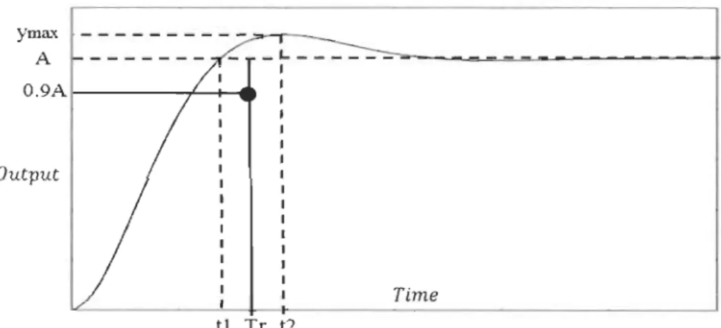
For a unit input value applied to the system, the output response will be recorded as shown in the figures 3.4, 3.5, 3.6. A O.9A Output O.lA 1
---#-1 1 Time t2
Figure 3. 4: Output response for real system with no overshoot
A
O.9A 1---+_....;.-....
Output
Time
t2 Tr t1
Figure 3. 5: Output response for real system with overshoot and oscillations.
ymax - - - -:::o-..--~ A - L - - - -.;;;-;.--....-.. ... .-...- - - -1 O.9At---"7'-_ _e Output Time t1 Tr t2
After recording the input value and the output response, the weighted elements of the black box system can be determined.
For simplicity, the first weighted element
1fJi
is 1 (unit input).'!/Ji
= 1The weighted element
'!/Jz
is determined directly from figure 3.4, 3.5, 3.6.'!/Jz
= AThe weighted element system gain \V5 is also directly determined from
'!/Ji
and'!/Jz
.
'!/Jz
A'!/Js
= - =-'!/Ji
1 (3.l) (3.2) (3.3)The weighted element
'!/J
3'
the projected rise time will be also determined from the output response figure 3.4 if the output response presents no overshoot.tz =
Ume at
a.9A (3.4)ti =
Ume at
a.lAAnd in figure 3.5 and 3.6, the first step is to draw the a.9A value. The projected rising time TT will be defined as the average time between ti and tz
(3.5) tz =
Ume correspondant to
YmaxThe weighted element
l/J6
which is the initial delay is also determined from the output response curve (figure 3.4, 3.5, 3.6):(3.6)
After finding the weighted elements If/l, 1f/2, 1f/3, 1f/5 and 1f/6, an approximation of a first order system with the same weighted elements will be determined. The weighted element
1fJ4
is the last element to be determined to find the final tuned first order transfer function.The approximate system will have the following transfer function type K
G (s) = _ _ e-SD
NA
s
+
xThe weighted element If/I is applied to this first order system.
From these three weighted elements.
K
-=A
x
Knowing that the rising time of a first-order transfer function is:
2.2
l/J3
=-X
This weighted element should coincide with that of the real system (black box). 2.2
- = T
x
TWe can then determine the constants K and x as follows:
(3.7)
(3.8)
(3.9)
(3.10)
2.2
x = -TT2.2
K=-A TT (3.12)Now, real and approximated systems have the same weighted elements If/l, 1f/2, 1f/3, 1f/5, 1f/6. The
approximated system of first-order transfer function will be.
K C(s)
= __
e-SDs+x
2.2
x = -TT2.2
K=-A TT (3.13)The last weighted element 1f/4 will be validated once the output of first-order is compared to
the real system output.
In
this case we say that both systems are similar.3.3 Application to different black box systems output
A. Case study 1 Cl
(s)
=s+l
S3+
5s
2+
17s
+
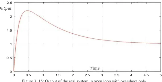
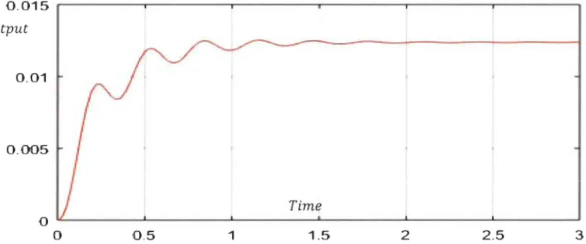
13 (3.14) Output 0.08 0.07 0.06 0.05 0.04 0.03 0.02 0.01 Time 1 2 3 4 5 6 7This output response will be used to find the approximated transfer function using the six weighted elements.
A unit input is applied to the real system. The steady-state of the output response is A
=
0.07691 and the three weighted elements are:
K
l/12
=
- =
x 0.07691l/12
Kl/1s
=
- = -
=
0.07691l/11
xThe weighted element 1f/3 related to the rising time will be determined as shown in figure 3.5. Then, the weighted element 1f/4 can be optimized at the same time.
2.2
t
l+
t
2l/J
3
=
~=
TT=
2=
0.7615From these equations, we can easily determine the parameters K and x.
x
=
2
.
2
=
2.889 ; K=
2.2
A=
0.2222TT TT
The weighted element \jf6 which is the initial delay will be determined directly from the output
response figure 3.5.
l/J6
= D = 0.07The first-order transfer function will be.
GNA(S) =
~e-SD
= 0.2222 e- SO.071 s
+
x s+ 2.889
(3.15)
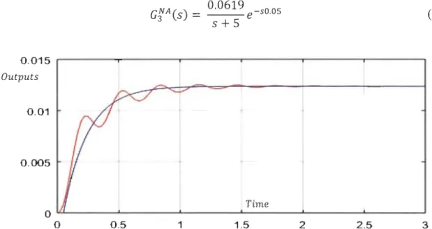
Simulation for comparison between the real and reduced open loop system is made (Figure 3.8).
Outputs 0.08 0.07 0.06 0.05 0.04 0.03 0.02 0.01 Time 1 2 3 4 5 6 7
Figure 3. 8: Output response of the real and reduced open-Ioop system.
One can see that both outputs coincide on ail elements 'lfl, 'lf2, 'lf3, 'lf4, 'lf5 and 'lf6. However,
the two curves do not absolutely coincide on the overshoot of the real system output, but this element is a low weighted element and will not influence the design of the closed loop controller. B. Case study 2 G2(s) = 0.5s
+
20 (3.16) S4+
10s3+
35s2+
50s+
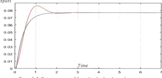
24 1 Output 0.8 0.6 0.4 0.2 Time 0 0 2 4 6 8 110 12 14Figure 3.9: Output response of the real open loop system with no overshoot.
A unit entry is applied to the real system, the steady-state of the output response IS A=0.8333. Then the three weighted elements are found as:
K
t/J2
= - =
0.8333l/J2
K
l/Js
= - = - = 0.8333l/Jl
x
The fact that the real system output does not have an overshoot, the element 1fJ3 is determined
using figure 3.4.
2.2 2.2
x
= - = 0.786; K = - A = 0.655Tr Tr
The element 1fJ6 which is the initial delay will be determined at the same time that 1f/4 is validated due to the nature of the output response (no overshoot).
l/J6
= D = 0.7 The first-order transfer function will be.0.655
GNA(S) =
e-
SO .72 S
+
0.786(3.17)
Simulation for comparison between the real and reduced open loop system is illustrated on figure 3.10. Outputs 0.8 0.6 0.4 0.2 Time
o
~~__
~______
~____
~~____
- L _ _ _ _ _ _ ~ _ _ _ _ ~ _ _ _ _ _ _ ~o
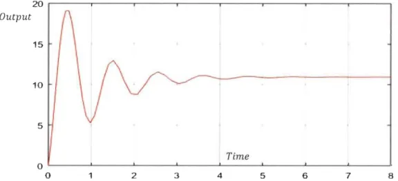
2 4 6 8 10 12 14C. Case study 3
0.5s
+
20G3 (s) = : : , ,
-S3
+
8s2+
420s+
1616(3.18)
This real system is a third order with an output response presenting oscillations with decreasing amplitude until its steady state regime as shown in figure 3.11. The approximate similar system will be the average first order using the weighted elements, especially 1f/3 the projected rising time.
0.015 r---r---~---~---~~---~---_,
Output
Time
1.5 2 2.5 3
Figure 3. Il: Output response of the real system with no overshoot with oscillations.
A unit input is applied to the real system, the steady-state of the output response is A = 0.01238 then the three weighted elements are also found:
K
lP2
= - =
0.01238 xlP2
K
lPs
= - = - = 0.0.1238lPl
x
The element lf/3 , the rising time is then determined. The real system output response presents sm ail oscillations, so the element lf/3 will be determined using figure 3.4.
2.2
![Figure 3. 14: Output response of the three systems- Real , reduced in [4] and proposed similar system](https://thumb-eu.123doks.com/thumbv2/123doknet/14611122.732453/57.918.188.790.183.450/figure-output-response-systems-real-reduced-proposed-similar.webp)