Patch-based models for image post-production

(1)

HAL Id: tel-01811035

https://hal.archives-ouvertes.fr/tel-01811035v2

Submitted on 2 Jul 2018

HAL is a multi-disciplinary open access archive for the deposit and dissemination of sci-entific research documents, whether they are pub-lished or not. The documents may come from

L’archive ouverte pluridisciplinaire HAL, est destinée au dépôt et à la diffusion de documents scientifiques de niveau recherche, publiés ou non, émanant des établissements d’enseignement et de

Patch-based models for image post-production

Aurélie Bugeau

To cite this version:

Aurélie Bugeau. Patch-based models for image post-production. Signal and Image Processing. Uni-versité de Bordeaux, 2018. �tel-01811035v2�

(2)

HABILITATION À DIRIGER LES RECHERCHES

Spécialité Informatique

Patch-based models for image post-production

Aurélie BUGEAU

Soutenue le 30 mai 2018 Membres du jury :

GILBOA Guy Maître de Conférences, Technion - Israel Inst. of Technology (rapporteur) LEZORAY Olivier Professeur, Université de Caen Normandie (rapporteur)

MASNOU Simon Professeur, Université Lyon 1 (rapporteur)

DOMENGER Jean-Philippe Professeur, Université de Bordeaux (Examinateur) KERVRANN Charles Directeur de recherche, INRIA Rennes (Examinateur) LEPETIT Vincent Professeur, Université de Bordeaux (Examinateur) THOLLOT Joëlle Professeur, Grenoble INP (Examinatrice)

(3)

(4)

À Nicolas, Esteban, Anaé

(5)

(6)

Résumé des activités de recherche

Ce chapitre décrit l’ensemble de mes activités de recherche depuis l’obtention de mon doctorat en 2007. Ces activités s’articulent autour de trois axes: l’estimation de données manquantes, la segmentation et le suivi d’objets, le traitement et l’analyse de vidéos pour les sciences humaines et sociales. Les chapitres suivants détailleront plus en détail le premier axe qui constitue ma thématique de recherche principale.

I - Estimation de données manquantes

Ma thématique de recherche principale concerne l’estimation de données manquantes à des fins de restauration d’images et vidéos ou de fusion d’informations multi-modales.

I.1 - Inpainting d’images et de vidéos

Ces recherches ont débuté lors de mon post-doctorat au sein de la fondation Barcelona Media de novembre 2007 à juin 2010 dans le cadre du projet espagnol i3media. Ce projet regroupant de nombreux partenaires universitaires et industriels, avait pour objectif la création et la gestion automatique de contenus audiovisuels intelligents. Plus précisément mon post-doctorat, encadré par M. Bertalmìo et V. Caselles, Pr Université Pompeu Fabra, Barcelone, traitait du problème de l’inpainting: étant donnée une image dégradée, il s’agit de reconstruire les zones abîmées de cette image de telle sorte que l’image finale ait l’air naturelle.

Inpainting d’images

Les méthodes de l’état de l’art peuvent être décomposées en deux catégories principales. Les méthodes de la première catégorie, communément appelées méthodes basées-patchs ou à patchs, reposent sur la comparaison de petites zones carrés de l’images. Plus pré-cisément, elles recherchent dans les zones non dégradées de l’image la couleur de sub-stitution des pixels dégradés, en fonction de leur voisinage (section 1.3). Ces méthodes s’adaptent très bien à des régions texturées (eau, herbe, sable ...) mais ne permettent pas

(9)

Résumé des activités de recherche de bien reconstruire les structures d’une image, c’est-à-dire les forts contours. La deuxième catégorie, qui a des propriétés inverses, regroupe les méthodes dites géométriques. Leur principe est de diffuser les couleurs connues sur le bord de la région à reconstruire vers l’intérieur de cette région en suivant les contours extérieurs (section 2.1.1). Aucune des méthodes existantes ne permet cependant de reconstruire correctement tout type d’image. Inspirés par (Bertalmio et al., 2003), nous avons tout d’abord proposer de combiner ces deux types d’approches en décomposant l’image à restaurer en la somme d’une image de texture et d’une image de structure. L’image de texture est tout d’abord reconstruite par une méthode à patchs tandis que l’image de structure est reconstruite par une méthode géométrique. L’algorithme mis en place donne de bons résultats sur une grande variété d’images mais reste trop dépendant de la méthode géométrique utilisée (Bugeau et al., 2009).

Nous avons par la suite combiné les deux types d’approches de manière plus directe. Ceci est fait en considérant une fonction d’énergie contenant trois termes principaux, un pour chaque type d’approche et un augmentant la cohérence entre pixels voisins. Cette éner-gie est minimisée de manière itérative sous un schéma multi-résolution. Cette méthode a permis d’obtenir des résultats encourageants sur un grand nombre d’images (Bugeau et al., 2010a). Elle a été étendue à l’inpainting d’images stéréo dans (Hervieu et al., 2010;

Hervieu et al., 2011). Inpainting de vidéos

J’ai par la suite étudié le problème d’inpainting de vidéos. La difficulté réside ici dans l’ajout de cohérence temporelle entre les reconstructions successives d’images. Pour que cette reconstruction ait l’air naturelle, il est indispensable de prendre en compte des in-formations sur le mouvement. Nous avons proposé une méthode basée sur un lissage de Kalman (Bugeau et al., 2010b). Les observations sont les images de la vidéo com-plétées une à une par une méthode d’inpainting d’image. Les prédictions sont obtenues en appliquant une méthode d’inpainting géométrique sur le flot optique entre deux frames successives .

I.2 - Colorisation d’images et de vidéos

Depuis 2012, je m’intéresse également à la colorisation d’images, i.e. à l’estimation des canaux de couleur de chaque pixel d’une image en niveaux de gris.

(10)

Résumé des activités de recherche

Méthodes à patchs pour la colorisation d’images

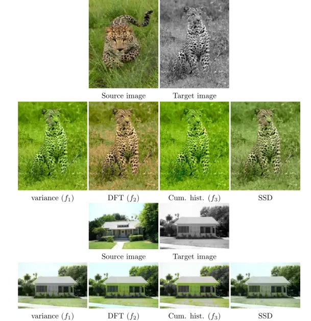
Il existe dans la littérature deux approches principales. La première se base sur la diffusion des couleurs : l’utilisateur choisit manuellement la couleur d’un certain nombre de pixels de l’image puis ces couleurs sont automatiquement diffusées aux pixels voisins (e.g. Levin et al., 2004, section 3.1). Cette méthode est limitée à des images simples contenant peu d’objets. Le second type d’approches concerne la colorisation dite par l’exemple. Elle est issue des méthodes de synthèse de texture à patch (Efros et al., 1999). Il s’agit ainsi de copier dans l’image en niveau de gris les teintes ou chrominances d’une image source en couleur (e.g. Welsh et al., 2002, section 1.4). L’avantage est que, mis à part la sélection de l’image couleur de référence, ces méthodes sont entièrement automatiques. Ces approches par l’exemple reposent sur la comparaison entre les luminances de l’image en niveau de gris et celles de l’image couleur. Cette comparaison est classiquement effectuée en calculant la (dis-)similarité entre le voisinage d’un pixel à coloriser avec l’ensemble ou un sous-ensemble des patchs de l’image couleur. De nombreuses métriques et descripteurs existent pour comparer des patchs mais aucune étude exhaustive portant sur l’influence de chaque métrique sur les résultats de colorisation n’a été publiée. Une des raisons est qu’il n’existe pas de mesure quantitative adaptée permmettant de valider les résultats de colorisation. Dans ce contexte, en collaboration avec V.-T. Ta, MCF LaBRI/Bordeaux INP, nous avons proposé une méthode permettant de calculer pour chaque pixel la meilleure couleur à lui transférer pour différents descripteurs d’un patch. Chaque pixel a ainsi plusieurs couleurs candidates possibles, une pour chacune des métriques. Dans (Bugeau et al., 2012), la sélection de la couleur finale se fait tout simplement en prenant la couleur médiane de l’ensemble des candidats possibles.

Modèles variationnels pour la colorisation d’images et de vidéos basée patch Nous avons par la suite, en collaboration avec N. Papadakis, CR CNRS/IMB, proposé la sélection automatique du meilleur candidat par une méthode variationnelle permettant l’ajout d’une contrainte spatiale sur la sélection (Bugeau et al., 2014). Ces travaux ont été poursuivis dans le cadre de la thèse de Fabien Pierre, dirigée par J.-F. Aujol, Pr Uni-versité de Bordeaux/IMB et co-encadrée par V.-T. Ta et moi-même (section 1.4.3). Une étude sur le calcul d’une combinaison linéaire optimale de métriques entre patchs pour la colorisation d’images a tout d’abord été menée (Pierre et al., 2015b). Il apparait, avec cette méthode, que le choix de la métrique optimale est trop dépendant de l’image à col-oriser et qu’une sélection au sein d’un modèle variationnel (Bugeau et al., 2014) apporte de meilleurs résultats. Nous avons donc poursuivi dans cette direction (chapitre 3). Un défaut majeur des résultats de colorisation existants est qu’ils sont globalement ternes.

(11)

Résumé des activités de recherche Nous avons analysé les raisons et proposés des solutions applicables à l’ensemble des méthodes de l’état-de-l’art. Lors de la colorisation d’images, l’image originale en niveaux de gris est considérée comme un canal de luminance et les couleurs sont créées en modifiant les deux canaux de chrominance. Le résultat luminance/chrominance obtenu est ensuite converti en RGB pour pouvoir être observé. Néanmoins les conversions des espaces de luminance/chrominance vers RGB ne permettent pas toujours de conserver correctement la teinte de l’image colorisée. La première solution que nous avons proposé consiste à travailler directement dans l’image RGB. Le modèle variationnel (Bugeau et al., 2014) a été modifié de façon à estimer une image RGB tout en respectant la contrainte de lumin-ance (luminlumin-ance de l’image finale égale aux niveaux de gris de l’image initiale) (Pierre et al., 2014b). Dans cette méthode, la projection de la couleur RGB estimée sous con-trainte de luminance est réalisée avec une projection orthogonale. Malheureusement cette projection ne conserve pas correctement la teinte de la couleur RGB initiale. Une étude approfondie des espaces de couleur et de leurs propriétés géométriques nous a amené à proposer une projection oblique menant à des résultats de colorisation faisant maintenant parti de l’état de l’art (Pierre et al., 2015c; Pierre et al., 2015a).

Similairement aux travaux sur l’inpainting, nous avons également travaillé sur la com-binaison des deux grandes catégories d’approches de colorisation d’images. Nous avons ainsi unifié dans un seul modèle les approches par l’exemple et les approches basées sur la diffusion de couleurs marquées par un utilisateur (Pierre et al., 2014a; Pierre et al., 2015a). Ces travaux ont fait l’objet d’un dépôt logiciel appelé “Colociel”. L’extension de ces travaux (section 3.2.1) à la colorisation de vidéos, obtenue avec l’ajout dans nos fonc-tionnelles d’un terme encourageant la cohérence temporelle sur les couleurs candidates, a enfin été proposée (Pierre et al., 2017b).

Application au rehaussement de contraste

Les travaux sur les espaces couleurs et sur la préservation de la teinte ont été étendus au problème de réhaussement de contraste suite à une collaboration avec G. Steidl, Pr. université de Kaiserslautern, Allemagne. La mesure du contraste est ici définie comme une moyenne pondérée des différences locales entre pixels voisins. Le réhaussement est alors obtenu par minimisation d’un modèle variationnel augmentant cette mesure de contraste par un facteur donné tout en préservant la teinte de l’image initiale (Pierre et al., 2017a;

(12)

Image initiale Image rehaussée

Figure 1: Résultats de rehaussement de contraste (Pierre et al., 2017a).

I.3 - Enrichissement et complétion de nuages de points LIDAR

La dernière application entamée dans le cadre de mes recherches sur l’estimation de don-nées manquantes concerne la densification de nuages de points LiDAR. Ces travaux sont réalisés en collaboration avec J.-F. Aujol et M. Brédif, chercheur à l’IGN. L’équipe MATIS de l’IGN a développé un système de cartographie mobile (MMS), équipé de détecteur laser (LiDAR), de capteurs optiques, d’un GPS et d’une centrale inertielle. L’objectif à terme est de construire des cartes 3D extrêmement précises des zones urbaines. Les acquisi-tions LiDAR fournissent des informaacquisi-tions de profondeur et de réflectance permettant la reconstruction d’un nuage de points 3D éparse de l’environnement, contenant des millions de points par minute d’acquisition. En complément, les capteurs optiques apportent de nombreuses images HD avec différents angles de vue.

Enrichissement des images optiques

Dans le cadre du post-doctorat de Marco Bevilacqua, nous nous sommes intéressés au couplage des nuages de points LiDAR avec les images optiques. Plus précisément, nous avons travaillé sur l’enrichissement des images optiques en leur ajoutant un canal de profondeur u et de réflectance r provenant des points LiDAR préalablement projetés sur les coordonnées des pixels de l’image optique (figure 2). Les nuages de points LiDAR (rSet uS) n’étant pas denses et ayant des coordonnées sous pixelliques dans l’image, l’estimation de la profondeur et de la réflectance en chaque pixel n’est pas directe. Nous avons donc proposé un modèle variationnel encourageant les contours de la reconstruction LiDAR à correspondre aux contours de l’image et s’assurant de la cohérence spatiale des valeurs de profondeurs (Bevilacqua et al., 2016) et de réflectances (Bevilacqua et al., 2017). Pour cela une carte de visibilité dans l’image v de chacun des points projetés est estimée. Complétion de nuages de points LiDAR

Dans le cadre de la thèse de Pierre Biasutti débutée en septembre 2016, nous nous sommes intéressés à la suppression d’objets non permanents de la scène tels que des objets en

(13)

Figure 2: Méthode d’enrichissement des images optiques à partir des données de réflect-ance et de profondeur issues du capteur LiDAR (Bevilacqua et al., 2017). mouvement ou des voitures garées. Pour cela nous avons proposé une représentation 2D en topologie capteur du nuage de points 3D. La segmentation de l’histogramme de cette nouvelle image permet ensuite d’extraire semi-automatiquement le masque des objets à supprimer. Une méthode d’inpainting géométrique a alors été proposée pour estimer la profondeur des zones occultées (Biasutti et al., 2017b;Biasutti et al., 2018,section 2.1.2). Création d’orthoimages à partir de points LiDAR

La complétion de nuages de points LiDAR peut également s’appliquer à la création d’orthoimages. Une orthoimage est une image de la surface terrestre exempte de toute distorsion, généralement acquise par des vecteurs satellites ou aériens. Dans le cadre du stage de Master 2 de Pierre Biasutti, nous avons proposé une méthode générant une or-thoimage de réflectance et de hauteur à très grande résolution (1cm) à partir des points LiDAR fournis par un système de cartographie mobile. La projection verticale (sur le sol) du nuage de points LiDAR sur une grille de pixels 2D étant éparse, des algorithmes d’inpainting sont appliqués afin d’obtenir une reconstruction dense des cartes de hauteur et de réflectance (Biasutti et al., 2016; Biasutti et al., 2017a,section 2.1.3).

(14)

II - Segmentation et suivi d’objets

Depuis mon doctorat, je m’intéresse également à la segmentation et au suivi d’objets. Dans l’ensemble de ces travaux, ce problème est vue comme un problème d’étiquetage, l’objectif étant d’attribuer à chaque pixel une étiquette "fond" ou "objet".

II.1 - Segmentation et suivi par coupe de graphes

Lors de ma thèse je me suis intéressée à la segmentation et au suivi temporel d’objets en mouvement. Dans ce cadre, une méthode reposant sur la minimisation d’une énergie par un algorithme de coupe minimale/flot maximal dans un graphe a été mise en place. Elle permet de suivre indépendamment chaque objet et regroupe les avantages d’une grande partie des méthodes de suivi existantes. La méthode ainsi créée est capable d’initialiser automatiquement les cibles et gère les entrées et sorties du champ de la caméra. Ceci est possible de part la prise en compte des détections externes d’objets dans l’énergie. D’autre part, la méthode est robuste aux changements d’illumination et aux changements de topologie des objets. Comme les méthodes de suivi par filtrage, la cohérence temporelle est basée sur l’utilisation dans la fonction d’énergie de la prédiction des objets. Enfin, une deuxième énergie multi-objets a été mise en place afin de séparer les objets ayant pu fusionner au cours de la première minimisation et permettre d’appréhender les problèmes d’occultation partielle (Bugeau et al., 2007; Bugeau et al., 2008a; Bugeau et al., 2008b). Cette méthode a néanmoins le défaut de nécessiter deux étapes. J’ai poursuivi mes recherches sur ce sujet et mis en place, en collaboration avec V. Caselles et N. Papadakis, un algorithme de suivi ne requérant qu’une seule minimisation pour tous les objet et étant capable de bien gérer les occultations partielles et globales. Pour cela un objet est divisé en deux parties : une région visible et une région occultée. Elles sont toutes deux suivies conjointement de part la minimisation d’une seule fonction d’énergie par un algorithme de coupe minimale/flot maximal (Papadakis et al., 2011,figure 3).

Application à l’indexation d’images

Ces recherches sur la segmentation par coupe de graphes ont été appliquées à l’indexation d’images avec une méthode reposant sur les sacs de descripteurs et les sacs de mots (Bag of Features and Bag of Words). Comme dans le cadre de la recherche textuelle, le principe des sacs de mots consiste à représenter une image par une distribution discrète des "mots visuels" qui la composent. Pour cela, des descripteurs visuels sont extraits localement des images puis quantifiés à l’aide d’un dictionnaire visuel obtenu par classification K-means. Ce dernier permet d’associer à chaque image un histogramme de ses descripteurs.

(15)

Figure 3: Résultat du suivi d’objets (Papadakis et al., 2011) sur une séquence de la base de données PETS 2001. Les couleurs sombres indiquent les parties visibles des objets suivis, les couleurs clairs indiquant les parties occultées.

Ces méthodes ont le défaut de ne pas tenir compte de l’information spatiale des images, ou plus précisément de la position dans l’image de chacun des descripteurs intervenant dans la construction de l’histogramme. Dans (Karaman et al., 2012;Benois-Pineau et al., 2012), nous avons donc proposé d’intégrer l’information spatiale explicitement au sein des descripteurs, c’est-à-dire avant la création de l’histogramme. Ces descripteurs sont des graphes multi-échelle obtenus par triangulation de Delaunay appliquées aux points SURF (Bay et al., 2006) de l’image.

Afin d’ajouter une information spatiale au moment de la construction de l’histogramme de mots visuels, l’utilisation de pyramides spatiales a été proposé dans la littérature (Lazebnik et al., 2006). Cette méthode, qui a largement contribué aux avancées dans le domaine de la recherche d’images, n’est néanmoins pas invariante aux transformations affines des images. Dans le cadre de la thèse de Yi Ren, co-encadrée par J. Benois-Pineau, Pr LaBRI/Université de Bordeaux, nous avons travaillé sur le découpage de l’image en régions cohérentes, chaque région étant ensuite représentée par son propre histogramme de mots visuels. L’histogramme global d’une image, appelé "Bag-of-Bags of Words", est alors obtenu par concaténation des histogrammes de chaque région. Pour segmenter les images en régions cohérentes, nous avons proposés des énergies ensuite minimisées par un algorithme de coupe minimale/flot maximal (Y. Ren et al., 2014b; Y. Ren et al., 2014a,

(16)

Résumé des activités de recherche figure 4).

Figure 4: Méthode pour la création des “Bag-of-Bags of Words” (Y. Ren et al., 2014b;

Y. Ren et al., 2014a).

II.2 - Segmentation par étiquetage de superpixels

Un autre travail de recherche sur la segmentation d’une image à partir d’une base d’images étiquetées à été proposé en collaboration avec R. Giraud, doctorant LaBRI, V.-T. Ta, N. Papadakis et P. Coupé, CR CNRS/LaBRI. Ce travail repose sur la décomposition de l’image en superpixels (petites zones connexes et de couleur homogène de l’image) avec la méthode SLIC (Achanta et al., 2012). En introduisant un algorithme rapide et robuste de mise en correspondances de “patch de superpixels” (appelés superpatch), nous sommes capables de classifier chacun des superpixels d’une image à segmenter (Giraud et al., 2017,

figure 5).

III - Traitement et analyse de vidéos pour les sciences

humaines et sociales

Ma troisième thématique de recherche est multidisciplinaire et repose sur plusieurs collab-orations avec des chercheurs de sciences cognitiques et de sciences humaines et sociales.

III.1 - Anonymisation fine de visages

J’ai débuté en 2013 une collaboration avec Maria-Caterina Manes Gallo, Pr en Sciences de l’Information et de la Communication à l’université Bordeaux Montaigne et rattachée au laboratoire MICA (Mediation, Information, Communication, Art). L’objectif était

(17)

Figure 5: Utilisation de la méthode SuperPatchMatch pour la segmentation d’images (Giraud et al., 2017).

de réaliser une dé-identification fine des visages présents dans une vidéo. Il s’agit de préserver l’anonymat des personnes tout en conservant au maximum les expressions du visage et de manière plus générale les signes de communications non verbaux. Pour réaliser ce travail, j’ai co-encadré G. Letournel, ingénieur d’étude, avec J.-P. Domenger, Pr. LaBRI/Université de Bordeaux, et V.-T. Ta. Dans un premier temps, nous avons étudié les méthodes de détection automatique de visages ainsi que de points caractéristiques sur les visages. Nous avons ensuite proposé une méthode de dé-identification fine sur image fixe reposant sur un lissage adaptatif du visage (figure 6). Les yeux et la bouche sont conservés car indispensables à la reconnaissance des expressions. Le nez est supprimé car il aide à la reconnaissance faciale mais pas à celle des expressions. Le reste du visage est lissé avec une force proportionnelle à la distance aux yeux et à la bouche. L’obtention du résultat est obtenu par minimisation d’un modèle variationnel.

La validation des résultats est une partie très importante de cette thématique de recherche. En effet, il faut s’assurer que les personnes sont effectivement correctement anonymisées mais également que leurs expressions sont préservées. Cette validation doit être faite par des humains mais aussi par des systèmes automatiques. Nous avons ainsi appliqué des algorithmes de reconnaissance de visages de l’état-de-l’art pour valider nos résultats. Il apparaît que le taux de reconnaissance passe de 86% avant anonymisation à 51% après (soit proche du hasard). Pour la validation humaine, nous nous sommes appuyés sur les connaissances en tests de perception de chercheurs en sciences cognitiques. Le co-encadrement d’un stagiaire avec V. Lespinet Najib, MCF IMS/ENSC a mené à la mise en place d’un protocole de test de perception pour la validation des résultats d’anonymisation de visages. Le test proposé évalue la reconnaissance de visage puis la reconnaissance des émotions. Il a été testé sur un panel de 22 sujets avec des résultats très prometteurs.

(18)

Figure 6: Chaîne de traitements pour l’anonymisation fine de visages (Letournel et al., 2015): (a) image initiale, (b) détection de visages et localisation de repères faciaux, (c) pondération du traitement des zones d’intérêts, (d) segmentation de la tête, (e) résultat du lissage adaptatif.

L’ensemble de ces travaux sur l’anonymisation fine de visages dans les image fixes ont été publiés dans (Letournel et al., 2015).

III.2 - Caractérisation visuelle des affects sociaux

En parallèle de ces travaux, j’ai travaillé sur la caractérisation visuelle des affects sociaux. Ce dernier projet a été réalisé de part l’encadrement du post-doctorant Zuheng Ming et en collaboration avec T. Shochi, MCF CLLE-ERSSaB/Université Bordeaux Montaigne et J.-L. Rouas, CR CNRS. Il fait suite aux nombreuses études déjà menées par T. Shochi sur la caractérisation sonore des affects sociaux chez des sujets japonais et français, de part l’étude des attitudes non spontanées telle que l’admiration, le dégoût, la séduction... Les attitudes étant très liées à la culture, l’objectif à terme est de mettre en avant des profils prototypiques des mêmes attitudes chez des acteurs japonais et des acteurs français afin de fournir les caractéristiques clés permettant de mieux comprendre et se faire comprendre lors de la communication en langue étrangère avec des natifs. L’intérêt est donc de pouvoir aider à l’apprentissage des langues. En effet, la communication repose sur du verbal (le parlé) mais aussi sur des aspects non verbaux (prosodie, gestuelle...). Une méconnaissance de ces aspects non verbaux peut mener à une mauvaise compréhension lors de l’immersion dans une autre culture (Shochi et al., 2016). Dans ce contexte, l’objectif ici était de trouver dans des vidéos des caractéristiques visuelles, sur le visage, communes à plusieurs acteurs jouant une même attitude. Les méthodes existantes sur la reconnaissance des expressions du visage reposent généralement sur l’estimation des “Facial Action Units”. Dans nos

(19)

Résumé des activités de recherche travaux nous avons proposé une méthode fusionnant différents descripteurs d’images pour la détection de ces descripteurs (Ming et al., 2015).

Ces recherches nous ont amené à établir une collaboration avec T. Nishida, Université de Kyoto, Japon, avec qui nous avons défini un scénario pour l’acquisition de vidéos de ces attitudes sur plusieurs personnes placées simultanément dans des environnements immersifs en réseau (Nishida et al., 2015).

(20)

Scientific Publications

Book Chapters

BC2. H. Boujut, A. Bugeau, J. Benois-Pineau – Visual search for objects in a complex visual context: what we wish to see – Chapter in Semantic Multimedia Analysis and Processing - Editors: E. Spyrou, D. Iakovidis, P.J. Mylonas - Publisher: Digital Imaging and Computer Vision, CRC Press, 2014.

BC1. J. Benois-Pineau, A. Bugeau, S. Karaman, R. Mégret – Spatial and multi-resolution context in visual indexing – Chapter 4 in Visual Indexing and Retrieval - Editors: J. Benois-Pineau, F. Precioso, M. Cord - Publisher: Springer, 2012.

International Journal

J13. P. Biasutti, J-F Aujol, M. Bredif, A. Bugeau – Range-Image: Incorporating sensor topology for LIDAR point clouds processing – Photogrammetric Engineering & Remote Sensing, 2018.

J12. R. Giraud, V.-T. Ta, A. Bugeau, P. Coupé, N. Papadakis – SuperPatchMatch: an Algorithm for Robust Correspondences of Superpixel Patches – IEEE Transactions on Image Processing (TIP), 2017.

J11. F. Pierre, J.-F. Aujol, A. Bugeau, V.-T. Ta – Interactive Video Colorization within a Variational Framework – SIAM Journal on Imaging Sciences, 2017.

J10. M. Bevilacqua, P. Biasutti, J-F Aujol, M. Brédif, and A. Bugeau, – Joint Inpainting of Depth and Reflectance with Visibility Estimation – ISPRS Journal of Photogram-metry and Remote Sensing, Volume 125, pages 16-32, 2017.

J9. F. Pierre, J.-F. Aujol, A. Bugeau, G. Steidl, V.-T. Ta, – Variational Contrast Enhancement of Gray-Scale and RGB Images – Journal of Mathematical Imaging and Vision (JMIV), Volume 57, pages 99-116, 2017.

(21)

Scientific Publications J8. F. Pierre, J.-F. Aujol, A. Bugeau, N. Papadakis, V.-T. Ta, – Luminance-Chrominance

Model for Image Colorization – SIAM Journal on Imaging Sciences, Volume 8, Issue 1, 2015.

J7. A. Bugeau, V.-T. Ta, N. Papadakis, – Variational Exemplar-Based Image Coloriz-ation – IEEE Transactions on Image Processing (TIP), Volume 33, Issue 1, 2014. J6. N. Papadakis, A. Baeza, A. Bugeau, O. D’Hondt, P. Gargallo I Piraces, V. Caselles,

X. Armangué, I. Rius, S. Sagàs – Virtual camera synthesis for soccer game replays. – Journal of Virtual Reality and Broadcasting, Volume 9, Issue 2012, 2013.

J5. N. Papadakis, A. Bugeau, V. Caselles – Image editing with spatiogram transfer – IEEE Transactions on Image Processing (TIP), Volume 21, Issue 5, May 2012. J4. N. Papadakis, A. Bugeau – Tracking with occlusions via Graphcuts – IEEE

Trans-actions Pattern Analysis and Machine Intelligence (TPAMI), Volume 33, Issue 1, Jan. 2011.

J3. A. Bugeau, M. Bertalmío, V. Caselles, G. Sapiro – A Comprehensive Framework for Image Inpainting – IEEE Transactions on Image Processing (TIP), Volume 19, Issue 10, Oct. 2010.

J2. A. Bugeau, P. Pérez – Detection and segmentation of moving objects in complex scenes – Computer Vision and Image Understanding (CVIU), Volume 113, Issue 4, April 2009.

J1. A. Bugeau, P. Pérez – Track and Cut: simultaneous tracking and segmentation of multiple objects with graph cuts – EURASIP Journal on Image and Video Processing - Special Issue on Video Tracking in Complex Scenes for Surveillance Applications, 2008(317278):1-14, 2008.

Preprints

P1. P. Biasutti, J-F Aujol, M. Brédif, A. Bugeau – Diffusion and inpainting of reflectance and height LiDAR orthoimages – HAL Preprint 01322822, 2017.

International Conferences

C24. P. Biasutti, J.-F. Aujol, M. Brédif, A. Bugeau. – Disocclusion of 3D LiDAR point clouds using range images – ISPRS Annals of Photogrammetry, Remote Sensing and Spatial Information Sciences, 2017.

(22)

Scientific Publications

C23. M. Bevilacqua, J.-F. Aujol, M. Bredif, A. Bugeau. – Visibility Estimation and Joint Inpainting of Lidar Depth Maps – Internationnal Conference on Image Processing (ICIP), 2016.

C22. F. Pierre, J.-F. Aujol, A. Bugeau, G. Steidl, V.-T. Ta. – Hue-Preserving Perceptual Contrast Enhancement – Internationnal Conference on Image Processing (ICIP), 2016.

C21. T. Shochi, J.-L. Rouas, Z. Ming, M. Guerry, A. Bugeau, E. Donna. – Cultural differences in pattern matching : multisensory recognition of socio-affective prosody – International Congress of Psychology, 2016.

C20. F. Pierre, J.-F. Aujol, A. Bugeau, V.-T. Ta. – A variational approach for color image enhancement – SIAM Conference on Imaging Science, 2016.

C19. F. Pierre, J.-F. Aujol, A. Bugeau, V.-T. Ta. – Luminance-Hue Specification in the RGB Space – Scale space and variational method in computer vision (SSVM), 2015. C18. G. Letournel, A. Bugeau, V.-T. Ta, J.-P. Domenger, M.C. Manes Gallo. – Face de-identification with expressions preservation – IEEE International Conference on Image Processing (ICIP), 2015.

C17. T. Nishida, M. Abe, T. Ookaki, D. Lala, S. Thovuttikul, H. Song, Y. Mohammad, C. Nitschke, Y. Ohmoto, A. Nakazawa, T. Shochi, J.-L. Rouas, A. Bugeau, F. Lotte, Z. Ming, G. Letournel, M. Guerry, D. Fourer– Synthetic Evidential Study as Augmented Collective Thought Process – Preliminary Report – International scientific conference for research in the field of intelligent information and database systems (ACIIDS), 2015.

C16. Z. Ming, A. Bugeau, J.-L. Rouas, T. Shochi – Facial Action Units Intensity Estim-ation by the Fusion of Features with Multi-kernel Support Vector Machine – IEEE International Conference on Automatic Face and Gesture Recognition Conference and Workshops (FG), 2015.

C15. F. Pierre, J.-F. Aujol, A. Bugeau, V.-T. Ta. – Collaborative Image Colorization – CPCV workshop - European Conference on Computer Vision, 2014.

C14. F. Pierre, J.-F. Aujol, A. Bugeau, N. Papadakis, V.-T. Ta – Exemplar-based color-ization in RGB color space – IEEE International Conference on Image Processing (ICIP), 2014.

(23)

Scientific Publications C13. Y. Ren, A. Bugeau, J. Benois-Pineau– Bag-of-Bags of Words Irregular Graph Pyr-amids vs Spatial Pyramid Matching for Image Retrieval – International Conference on Image Processing Theory, Tools and Applications (IPTA), 2014. - Best paper award

C12. Y. Ren, J. Benois-Pineau, A. Bugeau – A Comparative Study of Irregular Pyr-amid Matching in Bag-of-Bags of Words Model for Image Retrieval – International Conference on Image and Signal Processing (ICISP), 2014.

C11. A. Bugeau, V.-T. Ta – Patch-based image colorization – International Conference on Pattern Recognition (ICPR), 2012.

C10. S. Karaman, J. Benois-Pineau, R. Mégret, A. Bugeau – Multi-Layer Local Graph Words for Object Recognition – International Conference on Multimedia Modeling (ICMM), 2012.

C9. B. Delezoide, F. Precioso, P. Gosselin, M. Redi, B. Merialdo, L. Granjon, D. Pellerin, M. Rombaut, H. Jégou, R. Vieux, A. Bugeau, B. Mansencal, J. Benois-Pineau, H. Boujut, S. Ayache, B. Safadi, F. Thollard, G. Quénot, H. Bredin, M. Cord, A. Benoît , P. Lambert, T. Strat, J. Razik, S. Paris, H. Glotin, IRIM at TRECVID 2011: High Level Feature Extraction and Instance Search – TREC Video Retrieval Evaluation workshop, 2011.

C8. A. Hervieu, N. Papadakis, A. Bugeau, P. Gargallo, V. Caselles – Stereoscopic Image Inpainting using scene geometry–IEEE International Conference on Multimedia and Expo (ICME), 2011.

C8 G. Facciolo, R. Sadek, A. Bugeau, V. Caselles – Temporally consistent gradient do-main video editing – 8th International Conference on Energy Minimization Methods in Computer Vision and Pattern Recognition (EMMCVPR), 2011

C7. N. Papadakis, A. Baeza, X. Armangué, I. Rius, A. Bugeau, O. D’Hondt, P. Gargallo I Piraces, V. Caselles, S. Sagàs – Virtual camera synthesis for soccer game replays – Conference on Visual Media Production (CVMP), 2010.

C6. A. Bugeau, P. Gargallo, O. D’Hondt, A. Hervieu, N. Papadakis, V. Caselles – Co-herent Background Video Inpainting through Kalman Smoothing along Trajectories– Modeling, and Visualization Workshop, 2010.

(24)

Scientific Publications

C5. A. Hervieu, N. Papadakis, A. Bugeau, P. Gargallo; V. Caselles – Stereoscopic image inpainting: distinct depth maps and images inpainting – International Conference on Pattern Recognition (ICPR), 2010.

C4. A. Bugeau, M. Bertalmío – Combining texture synthesis and diffusion for image inpainting – International Conference on Computer Vision Theory and Applications (VISAPP), 2009.

C3. A. Bugeau, P. Pérez – Track and Cut: simultaneous tracking and segmentation of multiple objects with graph cuts – International Conference on Computer Vision Theory and Applications (VISAPP), 2008.

C2. A. Bugeau, P. Pérez – Joint Tracking and Segmentation of Objects using Graph Cuts – Proc. Conf. Advanced Concepts for Intelligent Vision Systems (ACIVS), 2007.

C1. A. Bugeau, P. Pérez – Detection and segmentation of moving objects in highly dynamic scenes – IEEE Computer Society Conference on Computer Vision and Pattern Recognition (CVPR), 2007.

National Conferences

CN8. R. Giraud, V.-T. Ta, A. Bugeau, P. Coupé, N. Papadakis – SuperPatchMatch : Un algorithme de correspondances robustes de patchs de superpixels – Reconnaissance des Formes, Image, Apprentissage et Perception (RFIAP), 2018.

CN7. P. Biasutti, J.-F. Aujol, M. Brédif, A. Bugeau – Estimation de visibilité dans un nuage de points LiDAR – Conférence Française de Photogrammétrie et de Télédétection (CFPT), 2018.

CN6. P. Biasutti, J.-F. Aujol, M. Brédif, A. Bugeau – Desoccultation de nuage de points LiDAR en topologie capteur – Gretsi, 2017.

CN5. P. Biasutti, J.-F. Aujol, M. Brédif, A. Bugeau – Diffusion anisotrope et inpainting d’orthophotographies LiDAR mobile – Reconnaissance des Formes et Intelligence Artificielle (RFIA), 2016.

CN4. F. Pierre, J.-F. Aujol, A. Bugeau, V.-T. Ta – Combinaison linéaire optimale de métriques pour la colorisation d’images – GRETSI, 2015.

(25)

Scientific Publications CN3. G. Letournel, A. Bugeau A., V.-T. Ta, J.-P. Domenger, M.C. Manes Gallo – An-onymisation fine de visages avec préservation des expressions faciales– Reconnais-sance des Formes et Intelligence Artificielle (RFIA) , 2014.

CN2. S. Karaman, J. Benois-Pineau, R. Mégret, A. Bugeau – Mots visuels issus de graphes locaux multi-niveaux pour la reconnaissance d’objets– Reconnaissance des Formes et Intelligence Artificielle (RFIA) , 2012.

CN1. A. Bugeau, P. Pérez – Sélection de la taille du noyau pour l’estimationà noyau dans des espaces multidimensionnels hétérogènes – GRETSI, 2007.

Research Reports

RR1. A. Bugeau, P. Pérez – Bandwidth selection for kernel estimation in mixed multi-dimensional spaces – Technical report, INRIA, RR-6286, 2007.

(26)

(27)

Introduction

The purpose of image post-production is to generate a modified image from an original one by recovering or adding missing information to the image in order to improve its visual quality or modify its style. It involves processes such as image restoration (i.e. denoising or deblurring), contrast or color enhancement, loss data completion, stylization, etc. Digital data post-production is a common problem in any field involving signal processing and applications may thus range from computational photography to medical imaging or satellite imaging.

Image post-production is generally an ill-posed problem. Indeed recovering missing or damaged data cannot be done without any prior assumption. Inspired by the studies made on the visual human system, many methods rely on the predictability or redundancy of images. The notion of redundancy in natural images appeared more than fifty years ago in the context of human vision (Attneave, 1954; Barlow, 1961). According to these studies, the visual system seeks to represent an image with the smallest possible number of information. This is made possible as there exist statistical dependencies across space in any natural image. In order to be efficient, the human visual system reduces these redundancies by removing the statistical dependencies.

Different types of redundancies are present in natural images, each of them leading to different approaches for automatic image processing. For details on natural image stat-istics we refer the reader to (Simoncelli et al., 2001). In particular, we can differentiate spatial and spectral redundancy. Local spatial redundancy means that there is a strong correlation between neighboring pixels, i.e. predictability in local image neighborhood. Spectral redundancies means that there is a strong correlation among the colors or the spectrum within an image. Another important type of redundancy, which will be at the core of this document, corresponds to the self-similarity principle, meaning that an image contains a lot of repetitions of local information (see figure 0.1).

Image redundancy is exploited in many image processing and analysis tasks. For image and video compression, it is only natural to compress the data by removing spatial and temporal redundancy. For denoising, today most powerful methods replace noisy areas

(28)

Introduction

Figure 0.1: Illustration of the self-similarity principle. An image contains a lot of repeti-tions of local information.

by averaging the values of other similar areas in the same image, thus exploiting the self-similarity principle. In the context of image retrieval, object detection or action recognition, the goal is to retrieve images or areas containing similar representations. Methods usually rely on local spatial redundancy but the self-similarity principle also happens to be useful (Shechtman et al., 2007).

In the field of image post-production, methods exploiting the self-similarity principle are often referred to as patch-based approaches or non-local approaches. The assumption ly-ing behind is that, similar to the human visual system, a computer is also able to predict missing data exploiting the visual redundancy present in a single image or across several similar images. All the works in this trend are inspired by Shannon’s work on modeling the English language. In (Shannon, 1948), a Markov model is used to generate an English text by computing the probability distributions of each letter given the previous ones in a large English text. Then, starting from a given letter (the seed), successive letters are found by sampling this Markov chain. This idea has first been extended to images in (Efros et al., 1999) for the purpose of texture synthesis. The texture is modeled as a Markov Random Field assuming that the probability distribution of brightness values for one pixel given the brightness values of its spatial neighborhood is independent from the rest of the image. The neighborhood is a square window called a patch. As we will see all along this document this work is at the origin of many others in various applications. A non exhaustive list of improvements that have been proposed in the literature is: study of similarities between patches, higher-level representation of patches, order in which the pixels (seeds) are sampled, introduction of geometric constraints for better sampling, use of non square window. Despite these various improvements, most patch-based methods remain one-path greedy algorithm: pixels are processed one after the others without be-ing further modified. This property leads to the well known growbe-ing garbage problem: errors are propagating from one pixel to the next. The only way to prevent this issue

(29)

Introduction

from happening is to consider multi-pass (or iterative) algorithms. The difficulty becomes to demonstrate the convergence of such algorithm. In order to better understand the behavior and convergence of the algorithms, problems are generally modeled as the min-imization of energy functions or solutions of partial derivative equations (PDE). Several energy functions will presented and discussed in this document.

While we will mention other applications of image post-production we will concentrate on image inpainting and image colorization. Inpainting aims at reconstructing a part of an image in a way that is not (easily) detectable by an ordinary observer. Image color-ization consists in turning a grayscale image into a color one that must seems natural. Additionally to these two applications that concern the restoration and retrieval of nat-ural images, we will also mention results concerning the completion of laser detection and ranging (LiDAR) clouds of points for orthoimages production and dense depth maps generation.

In chapter 1 we will see in details how the initial texture synthesis approach has been extended for the tackled applications. Chapters 2 and 3 study several models to solve the inpainting and colorization problems with non-greedy algorithms. Finally the last chapter concludes this presentation and opens several new perspectives of research.

(30)

Introduction

(31)

Chapter 1 Exploiting the self-similarity principle

for image post-production

Every natural image contains redundant information. The human visual system is able to use the redundant information within an image or from previously memorized images in order to predict the content of a missing part of the scene. In this chapter we will see how this behavior translates into algorithm for recovering missing data in the context of image post-production. We will concentrate on patch-based methods that consider the self-similarity principle, assuming that an image has a lot of repetitions of local information. While there is no clear definition of self-similarity, it is generally understood as follows: if any small template in an image can be approximated by one or several other small templates in that same image, then the image is self-similar. The small templates are generally considered to be small square windows, also called patches, but other less regular shapes may also be considered. In both cases, they are small image parts that capture local color statistics, texture and structure information.

In the context of image restoration and enhancement, the exploitation of patch redund-ancy started with the seminal work by Efros et al., 1999, for texture synthesis. We will detail this method in section 1.1, and the metrics that can be used to compare patches in section 1.2. This work is at the origin of a huge number of research for various ap-plications. A good survey for paper before 2009 is L.-Y. Wei et al., 2009, and for after is Barnes et al., 2017. Let us briefly mention some applications here, without going into details: denoising (with the famous NonLocal-Means algorithm from Buades et al., 2005), super-resolution (Freeman et al., 2002), stereo-matching (Scharstein et al., 2002; Lu et al., 2013), stylization (Bénard et al., 2013), style transfer (Elad et al., 2017; Frigo et al., 2016), segmentation and labeling (Coupé et al., 2011), optical flow estimation (Fortun et al., 2016), stereoscopic image inpainting (Hervieu et al., 2010; Hervieu et al., 2011) etc.

(32)

1.1. PATCH-BASED TEXTURE SYNTHESIS In this chapter, we will concentrate on applications to image inpainting (section 1.3) and colorization of grayscale images (section 1.4).

1.1 Patch-based texture synthesis

The seminal paper (Efros et al., 1999) presented a simple yet effective patch-based texture synthesis method. The objective is to generate a new texture image u : Ω → R3 _{from a} small texture sample uS : ΩS → R3 (figure 1.1).

Figure 1.1: Texture synthesis: the objective is to generate a new texture image from a small texture sample. Figure taken from L.-Y. Wei et al., 2009.

The texture is modeled as a Markov Random Field assuming that the probability distri-bution of brightness values for one pixel given the values of its spatial neighborhood is independent from the rest of the image. The neighborhood is a square window (patch) around the pixel and its size is a global parameter of the algorithm. The input of the algorithm is a set of sample image patches (all patches entirely belonging to the sample texture domain ΩS_{). The task is to select an appropriate patch within this set for each} of the unknown pixels so as to predict their value. This is done by computing a distance between the known neighborhood of an unknown pixel and each of the sample patches. The unknown pixel is filled-in with the value of the center of the most appropriate patch. In the following, let u : Ω → R3 _{be a color image (or u : Ω → R an intensity image) and} uS the sample grayscale or color image. We denote as Ψs(p) a patch centered at pixel p= (x, y), of size N = (2s + 1) × (2s + 1) such that

Ψs(p) = {p + k, k ∈ Ps}

with Ps = {(i, j), i = −s · · · s, j = −s · · · s}. For the sake of clarity we will equivalently

(33)

CHAPTER 1. EXPLOITING THE SELF-SIMILARITY PRINCIPLE FOR IMAGE POST-PRODUCTION

use the notation Ψs(p) and Ψ(p). We also denote as

Ψu_s(p) = (u(p1), · · · , u(pN)) , pi ∈ Ψs(p) (1.1) the vector of image values within the patch Ψs(p).

As described in (Demanet et al., 2003), the texture synthesis problem as just described is akin to finding the correspondence map (also called nearest neighbor field, NNF, in Barnes et al., 2009), ϕ : Ω → ΩS_{, that associates each pixel of the target domain Ω of the} image to a pixel from the sample domain ΩS _{such that}

ϕ(p) = argminq∈ΩSd(Ψu_s(p), ΨuS_s (q)) (1.2) where d is a distance between the image value of patches Ψs(p) and Ψs(q) centered at p and q respectively. Details on possible distances are discussed in section 1.2.

There have been many improvements to the initial patch-based method from Efros et al., 1999. We here briefly describe some common tools which are later used in this document. Patch-wise approaches The pixel-wise texture synthesis approach as just described is time consuming as synthesizing each pixel requires an exhaustive search among all pixels from the sample image. To speed up the process and better reproduce the input local structures, patch-wise methods synthesize entire patches instead of pixels (Efros et al., 2001; Kwatra et al., 2003; Criminisi et al., 2004; Lefebvre et al., 2005). The common default is the increasing amount of garbage regions and the necessity to add a blending stage to remove discontinuities between adjacent pacth copies.

Multi-resolution scheme Another trend for accelerating and improving texture syn-thesis algorithm is to incorporate it into a multi-resolution scheme. The unknown image is iteratively approximated using some guidance from coarse to fine levels (L. Wei et al., 2000; Drori et al., 2003).

Approximate Nearest Neighbor (ANN) Over the years, several other strategies have been proposed to accelerate directly pixel-wise approaches, mostly leading to ap-proximate nearest neighbor search (ANN). Note that all the methods in this trend have been extended to a multi-resolution scheme. While it is possible to accelerate exact nearest neighbor algorithms by avoiding any useless calculation (Xiao et al., 2011), the search remains quite inefficient in comparison to ANN. Among ANN methods we can

(34)

1.2. MEASURING SIMILARITY BETWEEN PATCHES mention tree-based techniques (L. Wei et al., 2000; Di Blasi et al., 2003; Olonetsky et al., 2012; He et al., 2012) or methods taking advantage of spatial coherence. These latter reduce the search space making the assumption that neighbor pixels in the output are likely to have neighbor correspondences in the input (Ashikhmin, 2001; Tong et al., 2002; Busto et al., 2010). The first such work (Ashikhmin, 2001) proposed to perform texture synthesis by looking for the best match for pixel p ∈ Ω not in all ΩS _{but only among} the set {ϕ(p + k) − k} of shifted candidates. The idea, as stated by the author, was to increase performance by not "starting the search process from scratch at each new pixel". In practice it also imposes a certain coherence in the mapping function ϕ which clearly improves the visual quality of many synthesis results. This approach was extended to k-coherence by Tong et al., 2002.

Exploiting spatial coherence, Barnes et al., 2009, proposed the now famous approximate nearest neighbor algorithm called patchmatch. The assumption made is that the corres-pondence map is most likely to be piece-wise constant. The algorithm has three steps: 1) random initialization of the correspondane map 2) propagation exploiting spatial coher-ence 3) random search to avoid getting stuck into local minima. Its convergcoher-ence rate to exact NN has been studied in (Arias et al., 2012).

1.2 Measuring similarity between patches

The underlying questions behind any patch-based methods are: i) how to find a discrim-inant and compact representation of the local statistics lying within a patch? ii) how to measure the similarity between these representations? In this section we only focus on the comparison between patches of pixels but other metrics have been designed for more complex templates. For instance, in (Giraud et al., 2017), we have designed metrics for patches of superpixels.

1.2.1 Patch-based descriptors

Many representations of patches have been proposed in the literature. Our goal here is not to make an exhaustive list but to mention the most famous ones and the ones used later in this document. It is important to highlight that the use of these representations highly depends on the targeted application, either we need to find color, texture or structure similarity.

The first low-level feature is the raw pixel intensity or color values themselves. This is the most widely used representation in patch-based methods.

In order to capture local color statistics, the mean and standard deviations of pixel values

(35)

within the patch is a very compact representation, though not highly discriminant. Higher dimensional representation are the intensity or color histograms, normalized histograms or cumulative histograms.

Several representations capturing frequencies of important structures can be obtained in the Fourier domain: Discrete Fourier Transform (DFT), Discrete Cosine Transfrom (DCT) for instance. The DFT is combined to other representation for image colorization in (Bugeau et al., 2012). In the same trend, Gabor filters have been used for image colorization in (Chia et al., 2011) and (Gupta et al., 2012).

A simple way to capture intensity or color variation within a template is to rely on image derivatives: intensity gradients and/or magnitude of gradients. Use of these features for image inpainting can be found in (Y. Liu et al., 2013) and (Newson et al., 2014). Higher order derivatives can also be considered. For instance region covariance (Tuzel et al., 2006) computed over the first and second intensity derivatives is used for colorization and color transfer in (Arbelot et al., 2016).

Finally, when measuring similarity across different images, it is often necessary to rely on scale, orientation and illumination invariant representations. Well known descriptors in this trend, built from gradient orientations, are SIFT (Lowe, 1999), SURF (Bay et al., 2006) or DAISY (Tola et al., 2008). These descriptors are well suited for matching highly structured image areas such as corners or keypoints. SIFT has been used for patch-based denoising (Lou et al., 2009) and colorization (Chia et al., 2011), and DAISY for image colorization (Cheng et al., 2015).

None of these representations is well suited for all possible types of textured, structured or uniform areas of natural images. This is mostly why, in the context of image restoration, most methods rely directly on raw pixel values.

In the following, the patch representation computed on Ψs(p) is denoted by Ψfs(p) and is stored as a vector of size N:

Ψf_s(p) = (f (p1), · · · f (pN)) , pi ∈ Ψs(p). (1.3) For instance in case the representation are the raw pixels themselves, we have

Ψf_s(p) = Ψu_s(p) = (u(p1), · · · u(pN)) , pi ∈ Ψs(p).

1.2.2 Similarity metrics

Many metrics exist to compute the similarity between patch representations. The most widely used for image restoration is the squared ℓ2 norm of the difference between patches,

(36)

1.2. MEASURING SIMILARITY BETWEEN PATCHES called sum of squared differences (SSD). For two pixels p and q, it is defined as:

dSSD(Ψu(p), Ψu(q)) = X

k∈Ps

ku(p + k) − u(q + k)k2.

A Gaussian weighted version, dSSDG is also sometimes considered (as in Efros et al., 1999) in order to give more importance to central pixels. Other classical measures include the ℓ1 norm of the difference between patches, known as the sum of absolute differences (SAD), or zero normalized cross-correlation.

Before going any further, let us analyze the influence of the SSD on an inpainting example. Figure 1.2, taken from (Bugeau et al., 2010a), demonstrates the limitation of the SSD when comparing textures. The textured patch P0is, in its overall appearance, very similar to P2. But, pixel-wise, as the SSD is computed, the difference between pixels at the same location in both patches is greater than the difference between the pixels in P0 and the average value of P0. Think of the difference between two sinusoids of average µ which are 180◦ _{out of phase: although they look exactly the same, their SSD is greater than} the SSD between either sinusoid and the constant function of value µ. This is why patch P4, which is rather uniform and does not resemble at all P0, is more similar in terms of SSD to P0 than P2 is to P0. This problem was later discussed in (Newson, 2014) with the following explanation. Assume two patches Q1 and Q2 made of i.i.d. pixels with a normal distribution N(µ, σ2_{) and a constant patch Q}

3, with the constant equal to µ. The SSD patch distance between Q1 and Q2 follows a chi-square distribution χ2(0, 2σ2) while the one between Q1 and Q3 follows χ2(0, σ2). Patch Q3 is therefore more likely to be chosen as the best candidate for patch Q1.

a) Original image b) Patch P0 c) Patch P1 d) Patch P2 e) Patch P3 f) Patch P4

Figure 1.2: Sum of squared differences between texture and smooth patches: dSSD(P0, P1) = 5290 ; dSSD(P0, P2) = 5443 ; dSSD(P0, P3) = 5416; dSSD(P0, P4) = 5070.

To cope with this problem, in (Bugeau et al., 2010a), we have defined a new similarity

(37)

CHAPTER 1. EXPLOITING THE SELF-SIMILARITY PRINCIPLE FOR IMAGE POST-PRODUCTION measure: dSSDB(Ψu(p), Ψu(q)) := 1 N dSSD(Ψ u_{(p), Ψ}u_{(q)) · d} H(Ψu(p), Ψu(q)) , (1.4) where, for a given pair of patches Ψs(p), Ψs(q), dH(Ψu(p), Ψu(q)) denotes the Hellinger distance: dH(Ψu(p), Ψu(q)) = v u u t1 − B X i=1 q ρp(i)ρq(i), (1.5)

where ρp, ρq are the histograms of the image u computed on the patches Ψu(p), Ψu(q), respectively, and B is the number of bins of the histograms. The Hellinger distance is a modified version of the Bhattacharyya probability density distance so that it satisfies the triangle inequality. In practice a histogram is computed on each patch by using 8 bins for each color dimension (i.e. 512 bins in case of color images). Let us comment on the rationale behind this choice for d, which combines the SSD and the Hellinger distance. While the Hellinger distance permits to distinguish a smooth patch from a textured one because they have different distributions, it is rotation invariant and we still need the SSD to permit distinction in that case. As later noticed by (Le Meur et al., 2012), when two patches have the same distribution, their distance dSSDB is zero. The authors therefore propose a variant to cope with this limit:

dSSDB(Ψu(p), Ψu(q)) := 1

N dSSD(Ψ

u_{(p), Ψ}u_{(q)) · (1 + d}

H (Ψu(p), Ψu(q))) . (1.6) This metric is also well adapted for patch-based image denoising (Ebdelli et al., 2013).

As mentioned before, we do not wish to draft an extensive list of all existing similarity metrics. Let us however mention that studies for comparing noisy patches, assuming known the noise model, have been conducted (Deledalle et al., 2012).

As for patch representation, the quality of a similarity metric often depends on the types of data and desired application. This is why most recent papers for image inpainting and image colorization prefer to rely on several types of patch representations thus defining new metrics to compute similarity between patches. We will discuss this matter later in this document.

(38)

1.3. FROM PATCH-BASED TEXTURE SYNTHESIS TO PATCH-BASED IMAGE INPAINTING

1.3 From patch-based texture synthesis to patch-based

image inpainting

Inpainting is the art of filling an unknwon area of an image or a video in a form that is not (easily) detectable by an ordinary observer. It has become a fundamental area of research in image processing with different applications: restoring missing image blocks (error concealment) in telecommunications, removing scratches or dust in movies, adding or removing elements in images or movies, and image extension. It is an old problem in art restoration as medieval artwork started to be restored as early as the Renaissance (as underlined in Bertalmio et al., 2000). In the art domain, it is also called retouching. The problem was brought to the image processing community by (Masnou et al., 1998) where it was named image disocclusion. The term inpainting was invented for art restorations (Emile-Male et al., 1976) and was first used for digital image restoration in (Bertalmio et al., 2000).

Inpainting is an ill-posed inverse problem which does not have a unique solution. A good solution is one that is undetectable by a human observer. To solve the inpainting problem, some priors must be considered. The commonly assumed prior is that any pixel in an image share the same geometrical and color statistics than its surrounding pixels (local spatial redundancy). Depending on the other priors considered, image completion tech-niques can be divided into three basic groups: 1) examplar-based or patch-based methods exploiting the self-similarity principle. Recent survey describing this category can be found in (Buyssens et al., 2015); 2) geometrical or diffusion-based methods considering a smoothness prior (see section 2.1.1); 3) hybrid methods combining the two previous types of approaches. Recent surveys describing all these categories can be found in (Bertalmío et al., 2011; Guillemot et al., 2014; Newson, 2014). We only focus in this section on the first category: patch-based methods for image inpainting.

Patch-based image inpainting methods, first introduced in (Bornard et al., 2002), all ex-tend the texture synthesis algorithm of Efros et al., 1999. The extension to inpainting is straightforward: given an image u defined on the set Ω with a hole H, fill-in each pixel inside H with a value (or combination of values) taken from the known area of the image ΩS _{= Ω \ H (see figure 1.3).}

Filling order Generally, layers of the unknown mask are inpainted successively in an onion peel strategy. As first highlighted in (Drori et al., 2003), the order with which

(39)

ΩS

H

Figure 1.3: Known and unknown areas for inpainting. Left: original area, Right: known area in white and unknown area in gray.

the pixels are filled strongly influence the results. Criminisi et al., 2004, designed a clever ordering procedure with priorities depending on edge strength. The priority order at a pixel is the product of a confidence term, which measures the amount of reliable information surrounding the pixel, and a data term, that encourages linear structures to be synthesized first. The confidence term is the ratio of the number of known pixels divided by the total number of pixels in the patch. The data term is defined as

D(p) = |∇u ⊥_(p).n

p|

α (1.7)

where ∇⊥ _{is the orthogonal gradient, α a normalization factor (equal to 255 for grayscale} images) and np a unit vector orthogonal to the inpainting area. It encourages the linear structures to be synthesized first and depends on the isophotes (contours) that eventually pass by p.

In (Bugeau et al., 2009), we have proposes a new data term based on the structure tensor (Di Zenzo, 1986) computed on the structure image after texture/structure decomposition (Vese et al., 2003). Stucture tensors were also used in the geometry-aware data term proposed in (Buyssens et al., 2015). In (Le Meur et al., 2011), the data term is modified to rely on structure tensor, which better captures the local geometry. In (Xu et al., 2010), a sparsity-based priority has been proposed in order to further improve the data term from (Le Meur et al., 2011).

Post-processing Despite all the great improvements made to patch-based inpainting (see chapter 2 for details on more advanced techniques), a common remaining problem concerns illumination discontinuities at the border of the mask. This problem may have two reasons: there are no candidate patches of the right color or the metric used is not adapted. To deal with this defect, as in (Sun et al., 2005), we have proposed in (Bugeau et al., 2010a) to add a post-processing step of Poisson image editing (Pérez et al., 2003).

(40)

1.4. FROM PATCH-BASED TEXTURE SYNTHESIS TO PATCH-BASED IMAGE COLORIZATION The final colors are obtained by solving:

min ˆ u

Z

H∪∂H

k∇ˆu− ∇u(ϕ(p))k2₂ with ˆu|∂H = u|∂H where ∂H is the outer boundary of H.

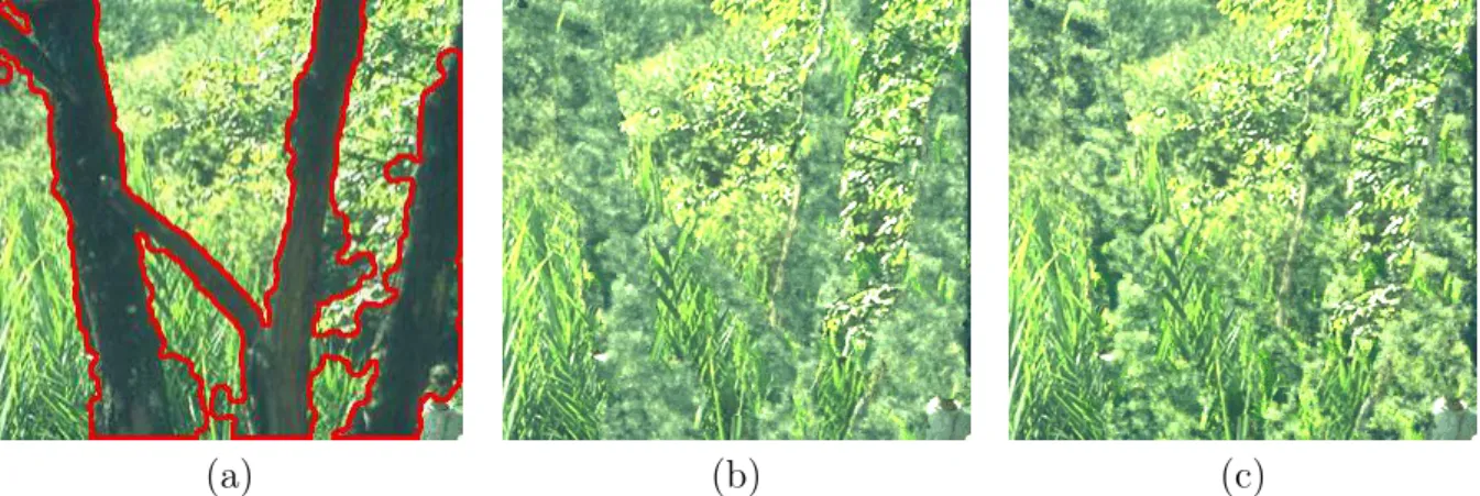
Other post-processing approach relies on color histogram equalization, which is a well known tool for contrast enhancement (Kim, 1997; Nikolova et al., 2014;Pierre et al., 2016). Nevertheless, as histograms do not include any information on the spatial repartition of colors, their application to local image editing problems remains limited. To cope with this lack of spatial information, spatiograms have been proposed for tracking purposes (Birchfield et al., 2005). A spatiogram is an image descriptor that combines a histogram with the mean and variance of the position of each color. In (Papadakis et al., 2012), we have addressed the problem of local retouching of images by proposing a variational method for spatiogram transfer. More precisely, a reference spatiogram, computed on ΩS is used to modify the color values within H of a given region of interest of the processed image. From figure 1.4, we can see that the spatiogram transfer allows correcting the default of patch-based inpainting results while preserving the textures. This combination produces really plausible reconstructions (see Fig. 1.5(c) for details on the tree example).

1.4 From patch-based texture synthesis to patch-based

image colorization

Image colorization consists in recovering a color image from a grayscale one. This ap-plication attracts a lot of attention in the image-editing community in order to restore or colorize old grayscale movies or pictures. While turning a color image into a gray-scale one is only a matter of standard, the reverse operation is a strongly ill-posed problem as no information on which color has to be added is known. Therefore priors must be added. In literature, there exist two kinds of priors leading to two different types of colorization methods. In the first category, initiated by Levin et al., 2004, the user manually adds initial colors through scribbles to the grayscale image. The colorization process is then performed by propagating the input color data to the whole image (section 3.1). The second category, called automatic or patch-based colorization, consists in transferring color from one (or many) initial color image considered as example.

For both, the initial grayscale image is considered as the luminance channel which is not

(41)

(a) (b) (c)

Figure 1.4: Patch-based inpainting correction with spatiogram transfer. (a) Original im-age and the inpainting mask in red. (b) Result obtained with (Criminisi et al., 2004) using patches of size 9 × 9. (c) Post-processing result obtained in (Papadakis et al., 2012).

(a) (b) (c)

Figure 1.5: Patch-based inpainting correction with spatiogram transfer (Papadakis et al., 2012). (a) Zoom on the original image of the second row of figure 1.4 (b) Zoom on the patch-based inpainting result. (c) Zoom on the corresponding spatiogram transfer correction which produces really plausible reconstructions .

modified during the colorization. The objective is then to reconstruct the two chrominance channels, before turning back to the RGB color space. Different luminance-chrominance spaces exist and have been used for image colorization: lαβ (Ruderman et al., 1998) as in (Welsh et al., 2002), Lab as in (Charpiat et al., 2008), YCbCr as in (Yatziv et al., 2006), or YUV as in (Bugeau et al., 2012). In all of our works, we have used the YUV space

(42)

1.4. FROM PATCH-BASED TEXTURE SYNTHESIS TO PATCH-BASED IMAGE COLORIZATION since its conversion to RGB is linear.

1.4.1 General pipeline for patch-based image colorization

The first patch-based colorization method was proposed by Welsh et al., 2002. It makes the assumption that pixels with similar intensities or similar neighborhood should have similar colors. It extends the texture synthesis approach by Efros et al., 1999: the final color of one pixel is copied from the most similar pixel in the input color image. The similarity between pixels relies on patch-based metrics. This approach has given rise to many extension in the literature.

In the following, we denote as

• uT : Ω → R the target grayscale image (which is assumed to be a luminance image) • u : Ω → R3 _{the estimated color image, Y}

u : Ω → R its luminance (that must be equal to uT), uc = (Uu, Vu) : Ω → R2 its chrominances in the YUV color space, and Ru, Gu, Bu its channels in the RGB color space.

• uS : ΩS → R3 the source color image.

With these notations, the goal of image colorization is to find u under the constraint that it luminance channel Yu is equal to uT. Most patch-based methods for image colorization proposed in the literature can be summarized into a three-steps general pipeline.

Step–1, Pre-Process uS and uT

This step consists in converting uSto a luminance-chrominance space and setting Yu = uT. Automatic patch-based image colorization methods rely on a copy/paste of the chromin-ances from the source image to the target image. In order to select the color to transfer, the luminance of uS ( denoted by YuS) and uT should be comparable. Ideally, the transfer process should take into account the global difference in luminance of the two images, i.e., these two images should have similar global statistics such as the mean and the variance. For this purpose, an affine luminance mapping (Hertzmann et al., 2001) is generally per-formed on YuS.

Step–2, Predict Color from uS and transfer to u

The second step aims at choosing for each pixel p ∈ Ω the best pixel ϕ(p) ∈ Sn which minimizes a distance on the luminance neighborhoods:

ϕ(p) = arg min q∈Snd(Ψ

Yu_{(p), Ψ}YuS_{(q)) .}

The process is illustrated on figure 1.6. The set Sn = {q1, . . . , qn} of n possible candidate pixels is either the whole pixel grid ΩS _{of the source image or a subset of this grid}