RESEARCH OUTPUTS / RÉSULTATS DE RECHERCHE
Author(s) - Auteur(s) :
Publication date - Date de publication :
Permanent link - Permalien :
Rights / License - Licence de droit d’auteur :
Institutional Repository - Research Portal
Dépôt Institutionnel - Portail de la Recherche
researchportal.unamur.be
University of Namur
Robustness of artificial neural network and discrete choice modelling in presence of
unobserved variables
Dumont, Morgane; Barthelemy, Johan; Carletti, Timoteo
Published in:
Proceedings - 22nd International Congress on Modelling and Simulation, MODSIM 2017
Publication date:
2017
Link to publication
Citation for pulished version (HARVARD):
Dumont, M, Barthelemy, J & Carletti, T 2017, Robustness of artificial neural network and discrete choice modelling in presence of unobserved variables. in G Syme, DH MacDonald, B Fulton & J Piantadosi (eds),
Proceedings - 22nd International Congress on Modelling and Simulation, MODSIM 2017: Modelling and Simulation Society of Australia and New Zealand. Proceedings - 22nd International Congress on Modelling and
Simulation, MODSIM 2017, pp. 480-486. <https://www.mssanz.org.au/modsim2017/C6/dumont.pdf>
General rights
Copyright and moral rights for the publications made accessible in the public portal are retained by the authors and/or other copyright owners and it is a condition of accessing publications that users recognise and abide by the legal requirements associated with these rights. • Users may download and print one copy of any publication from the public portal for the purpose of private study or research. • You may not further distribute the material or use it for any profit-making activity or commercial gain
• You may freely distribute the URL identifying the publication in the public portal ?
Take down policy
Robustness of artificial neural network and discrete
choice modelling in presence of unobserved variables
M. Dumonta
, J. Barth´elemyb
and T. Carlettia a
naXys, University of Namur
b
SMART, University of Wollongong
Email:[email protected]
Abstract: Models are used to gain a better understanding of complex systems such as the evolution of a population, the transportation demand, the brain behaviour, elections outcome, the propagation of a disease,... System models should be precise and parsimonious. However, the total variation of the system cannot be precisely captured by the observed variables as there can be unobserved ones influencing the system output. The unexplained variation caused by unobserved variables is, therefore, considered as a noise in the model. Different models handle that noise in a different way. For instance, a linear regression assumes that the noise follows a normal distribution and explicitly incorporates it into the model formulation. On the other hand, other models, such as a deterministic neural network, do not explicitly incorporate that noise. Several models can then be applied and the selection of the best one can be a challenging question.
This research aims to highlight the importance of the unobserved variables on the results of two types of simple yet widely used models: feedforward neural networks (FFNN) and logit discrete choice models (LDCM). The first application consists in modelling the divorces in an agent-based microsimulation, the agents being the individuals of a given population. For each couple in the model, the divorce is predicted based on the characteristics of the couple (ex: length of the marriage, age of the individuals). In this application, it is shown that the LDCM outperforms the neural network due to the presence of - possibly many - unobserved variables. The second example is a model defined to predict the level of interaction between groundwater and quarry extensions. In this application, the value of every relevant variable is assumed to be known, i.e. the noise from unobserved variables is minimum. In this case, it is shown that both approaches perform well, but FFNN perform slightly better than LDCM. We then investigate how the model performance evolves when the noise increases by removing variables from the models specification.
Finally, those two applications will allow us to conclude on the robustness of the discrete choice models and artificial neural network in presence of unobserved variables.
Keywords: Discrete choice modelling, neural network, unobserved variables
M. Dumont et al., Robustness of artificial neural network and discrete choice modelling ... 1 INTRODUCTION
Models are used to gain a better understanding of complex systems such as the evolution of a population, the transportation demand, the brain behaviour, elections outcome, the propagation of a disease,...
System models should be precise and parsimonious. However, the total variation of the system cannot be precisely captured by the variables observed as there can be unobserved variables influencing the system. The unexplained variation caused by unobserved variables is, therefore, considered as a noise in the model. Different models handle that noise in a different way. For instance, a linear regression assumes that the noise follows a normal distribution and explicitly incorporates it into the model formulation. On the other hand, other models, such as a deterministic neural network, do not explicitly incorporate that noise. Several models can then be applied and the selection of the best one can be a challenging question. This research aims to highlight the importance of the unobserved variables on the results of two types of simple yet widely used models: feedforward neural networks (FFNN) and logit discrete choice models (LDCM).
The first aim of this paper is to apply FFNN and LDCM, on a real life application: simulating the divorces for the married couples in Belgium. The paper is structured in five sections. First, the available data are exposed in Section 2. Secondly, we develop logit discrete choice modelling, by explaining the bases of the theoretical concept before to apply it on the divorces in Section 3. Then, the Section 4 outlines the domain of feedforward neural networks theoretically and then apply it to divorces. Section 5 explains the impact of unobserved variables thanks to the data of Barth´elemy et al. [2016a] that compare both methods (FFNN and LDCM) on the specific case of classifying quarries in different levels of interaction with groundwater. The authors disposed of all pertinent information useful to the classification and both methods gave satisfactory results. To analyse the impact of unobserved variables, the outcomes of the models can be tested once we gradually and artificially reduce the information content, i.e. removing relevant variables. Finally, we conclude and propose suggestions to continue this work.
2 DATA
Since 1983, each citizen of Belgium is registered in the municipality she is living in, with several information about himself: gender, date of birth, address, people he is living with, marital status, ... This database is called the National Register. When a change occurs in a variable describing the citizen status, the latter needs to notify the municipality. There is a longitudinal recording of the data, that allows to move back in time and analyse different years or different specific path (for example, time between weddings and divorces, or the first moves after a wedding,...).
To model divorces, the choice made in 2002 (either divorce or stay together) by each couple still married in 2001 is recorded. In addition, each couple is characterised by : year of the wedding, size of household in 2001, age class of the husband and spouse, diploma level of both, subjective health level of both and province they are living in in 2001. This results in approximately one million couples with 8000 divorcing in 2002 (corresponding thus to 0.8% of the couples divorced).
To test the methods, we separate randomly the database in two parts : one part is the calibration set, that will be used to calibrate both methods (FFNN and LDCM); the other part is the validation set. Both calibrated models will be tested on these data to check the prediction quality of the simulations. We split the data in 50% for calibration and 50% for validation using a simple random sampling scheme. We chose to keep a consequent part in the validation, because we have very few divorces in the whole data. Indeed, this already makes only approximately 4000 divorcing couples in the validation to have the possibility to check the attributes of the simulated divorcing couples.
3 LOGIT DISCRETE CHOICE MODELLING
3.1 Theoretical concept
Ben-Akiva and Lerman [1985] present the concept of discrete choice modelling. This method is to model the choice of individuals among different alternatives (mutually exclusive and exhaustive). For example, a common use of this theory was to describe travel behaviour and then forecast the mode of travel.
The theory behind this modelling assumes that each individual chooses the alternative that makes him the happiest (in economical terms, that maximises his utility). The exact utility of each possible choice is only known by the considered individual. The models try to approximate these utilities, but there is still a difference between the real utility U and the simulated utility V . This deviation is called the error, ǫ. The richness of this
domain is that it splits the utility in two terms: the observable factor (the ones included in the data concerning the alternative and/or the person), V and an unobservable factor, ǫ. Thus, the utility of an alternative a for the ithindividual is Uia= V a i + ǫ a i.
The observable part, Via, in linear models is defined as the linear combination of pertinent variables available in the data, weighted to best fit the calibration data. This observable part can be calculated after calibration and is the same for all individuals characterised by the same attributes. Different types of models have distinct assumptions on the random term ǫa
i of the model based on its density function. Knowing the observable utility and the distribution of the error, the model calculates a probability for each alternative choice of a person. Since an alternative is chosen if its total utility is higher than utilities of each alternative choice, the probability that individual i chooses alternative a is
Pia= P (Uia > Uib, ∀b 6= a) = P (Via− Vib > ǫbi − ǫai ∀b 6= a)
The Logit modelling considers the random terms ǫai as independent and identically distributed following a standard Gumbell law. The associated cumulative distribution is defined by F(ǫa
i) = e−e −ǫ
a i
(with e the Euler’s constant). This specification ensure a simple form of the probability of each alternative (Ben-Akiva and Lerman [1985]): Pia = eVia X k eV k i
Train [2009] or Ben-Akiva and Lerman [1985] provides more details about discrete choice modelling method-ology.
3.2 Modelling divorces using LDCM
The logit discrete choice modelling is developed to simulated the divorces in Belgium. The used data are discussed in Section 2. Note that this setting results into a binary logit since there is only two possibilities (exhaustive and mutually exclusive): divorce or stay together. Since only the difference of utility matters, we decide to fix the utility of staying together to zero.
The used model being linear on the variables, several operations on the input variables has been tried. First, we recategorised each ordinate variable into integers. For instance age’s intervals has been numbered from 1, for 15-19, up to 17, for 95-100 and more. We also normalised the input data (dividing each variable by its maximum). In a second phase, each variable has been transposed into boolean variables (1 if the attribute holds true, 0 on the contrary). This specific operation allows to capture non linear relations. This process shows that the age of the woman improves the model when being boolean, whereas it removes the significance of all categories of the age of the man. Therefore, the age of the wife is considered as boolean, but not the one of the husband. To calibrate and validate discrete choice models, we use BIOGEME (Bierlaire [2003]). The selected model has an adjusted ρ2
of 0.94, which means that the model fits well the calibration data. Note that a couple is characterised by several objects that occurs in the model: a woman (W ), a man (M ), an household (HH) and a marriage (M ar). The concerned characteristic is written as an index. For example Mage is the man’s age. Remember that the age of the woman is considered as boolean, implying that W3 stands for a woman of age between 25 and 29 (class 3). This final model is (remember Ustay= 0):
Udiv = 2.04W3+ 1.78W4+ 1.72W5+ 1.65W6+ 1.27W7+ 0.64W8 −0.56W10−1.01W11−1.67W12−1.83W13−0.41W14
−0.12Mage−0.13Mdipl−0.08Wsubj−health−0.14HHsize−0.02M arlength
Note that to facilitate the interpretation of this utility, all positively influencing terms are written at the begin-ning of the expression. We observe that the model found a linear correlation between the age category of the man in the couple and the proposition of divorce with a negative coefficient and a non linear relation for the age of the woman. Indeed, the coefficient changes from one age category to another. We can also note that the health of only the wife and the diploma of only the husband enter into account. Moreover, with the years of marriage and the number of children, the utility of divorce decreases. This model is used to simulate the
(1)
(2)
(3)
M. Dumont et al., Robustness of artificial neural network and discrete choice modelling ...
choices of the couples in the validation data. The probability to divorce is calculated for each couple. Then, 500 simulations are generated and their outcome are compared to the real choice of this couple.
Figure 1. Density of the number of simulated divorces using the discrete choice modelling (500 simulations)
Figure 1 shows the distribution of the number of divorce resulting from the 500 simulations. We can see that each run contains at least 3600 divorces and no more than 4000 with a mean of 3797, which is very close to the real number of divorces in the validation data set. The Z-test checking if the proportions of divorces are similar in the average simulation and in the reality has a p-value of 0.9222 meaning that the proportion of couples choosing to divorce is well defined in the model.
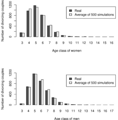
Figure 2. Bar chart of the number of divorces per age class and per gender (real vs simulated)
Figure 2 presents how the number of divorces distribute among the age classes of wife and husband (class 3 is 25-29 years old, ...), where actual number of cases are represented in black and the model results are shown in grey (the average number amongst the 500 generations). Figure 2 confirms that the actual pattern is well conserved in the model results as both black and grey bars are approximately of the same height. A T test with as null hypothesis ”The differences between the real and the average number has a mean of 0” confirms this intuition (p-value of 0.91 for women and 0.87 for men).
4 FEEDFORWARD ARTIFICIAL NEURAL NETWORK
4.1 Theoretical concept
An artificial neural network (ANN) is an algorithm that mimics the biological brains with their neurons and connections. In ANN, the inputs are fed to the network, pass through various layers of neurons (depending on the activation function of said neurons), and finally generate outputs. ANN at least contains two layers: inputs and outputs, but several layers of different number of nodes (neurons) can be added between these two layers. From one layer to the other, a weighted linear combination of the neurons in previous layer is performed and passed into an activation function. It should be noted that the number of layers, the number of neurons per layer and the connections between the layers define the architecture of the ANN. We choose here to develop a feedforward ANN, meaning that the signal only move in one direction: from input to the output. Details on artificial neural networks are available in Basheer and Hajmeer [2000], Agatonovic-Kustrin and Beresford [2000], Ripley [2007] or Kriesel [2007].
As with discrete choice modelling, the calibration step determines the parameters of the network, using a part of the data. The calibration (or learning/training) process of network’s parameters is stochastic in the sense that it starts with random values. This means that different initial values can lead to different networks. Hence training the network for several times using different set of initial value is needed to assess the robustness of the retained architecture. When the network is well calibrated, new inputs can be inserted to generate the forecast outputs. Although the calibration is stochastic, the forecasted outputs are deterministics.
4.2 Modelling divorces using FFNN
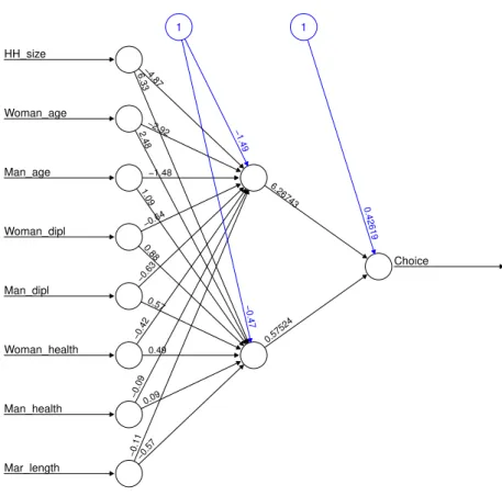
To generate the results, we use the R-package neuralnet (Fritsch et al. [2010]). Figure 3 illustrates the resulting network for the divorces.
−0.57 −0.11 Mar_length 0.09 −0.09 Man_health 0.49 −0.42 Woman_health 0.57 −0.63 Man_dipl 0.88 −0.64 Woman_dipl 1.09 −1.48 Man_age 2.48−2.92 Woman_age 6.33−4.87 HH_size 0.57524 6.26743 Choice −0.47 −1.49 1 0.42619 1
M. Dumont et al., Robustness of artificial neural network and discrete choice modelling ...
The inputs are the normalised attributes of the couples and the choice is a boolean output deciding if this couple divorces or not. One hidden layer of 2 nodes is included and the threshold for the activation function are shown in blue. When using this network to forecast the divorces for the validation data, the correct choice is made for 99,2% of the couples.
This seems to be a very good prediction rate, but we need to go further to see if the divorcing couples have the right characteristics. Trying to analyse this, we figure out that no couples will divorce with this model. Indeed, it predict that all couples will stay together. Since only a very small number of the couples actually divorce (0.8%), this makes a good prediction rate.
Many different configurations in terms of number of layers and nodes of the neural network have been tried to find a better artificial neural network. Zur et al. [2009] shows that noise injection can reduce overfitting. So, random noise has been added to the input and to the output in the calibration step. We also tried to add a random input neuron. Moreover, to calibrate the mean and standard deviation of these Gaussian noises, a genetic algorithm was realised. However, no divorcing couples appeared.
We figure out that in the data, many couples have exactly the same attributes, but don’t make the same choice. In each possible type of couple, the majority stay together and a few decide to divorce. Simulations with a calibrated neural network being deterministic, it returns the same output for each similar couple. We could consider the results as a probability, because it corresponds to the proportion of divorcing couples in the category. However, we don’t need a neural network to consider proportions as probabilities.
5 IMPACT OF UNOBSERVED VARIABLES
Discrete choice modelling being stochastic, it deals well in presence of latent variables. This section will focus on the robustness of ANN to unobserved variables.
Barth´elemy et al. [2016a] designed two indices to predict the interaction between extractive activity and groundwater resources using discrete choice modelling and artificial neural network approaches. The used data are freely available at Barth´elemy et al. [2016b] and contains six variables describing the quarry: the geological, hydrogeological and piezometric contexts (to catch the hazard that the quarry represents) and the relative position of the quarry and the water catchments, the production of the catchments and the potential quality of the groundwater, catching the vulnerability of the groundwater resource. We observed that two quarries having the same characteristics have necessary the same output index in the data. In the case of the divorces, this isn’t true, because of unobserved variables, such as for example the happiness of the couple.
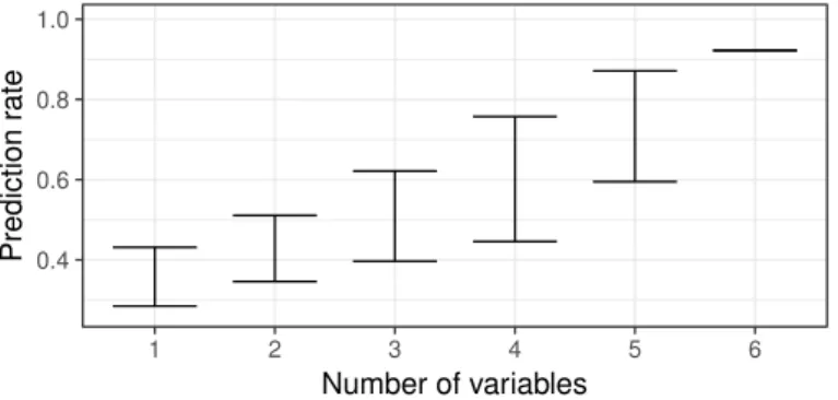
0.4 0.6 0.8 1.0 1 2 3 4 5 6 Number of variables Prediction r ate
Figure 4. Benchmark of the influence of unobserved variables
Discrete choice modelling being stochastic and returning probabilities of an alternative is more robust to unobserved variables. Indeed, if the calibration data contains individuals represented by exactly the same attributes, but making different choices, it will, on average, maintain the same proportion of entities making each choice. Our first test was to calibrate neural networks for the quarries without all attributes. We first took each variable separately, then each possible combination of 2 variables, etc. Figure 4 illustrates the minimum and maximum prediction rate depending on the number of included input variables. We can clearly see that the quality of the prediction becomes always smaller when the number of variables decreases. This means that neural network doesn’t perform well in presence of unobserved variable. Of course, this would be the case of all deterministic methods that generate exactly the same output when inserting two times an equivalent input.
6 CONCLUSIONS ANDRECOMMENDATIONS
In conclusion, discrete choice modelling enable us to forecast the divorces, with quite satisfactory results. Indeed, the simulated divorcing couples characteristics fit to the theoretical ones. It is a stochastic method, meaning that simulating twice doesn’t necessary give the exact same results. Artificial neural networks doesn’t return good results. This is caused by a presence of unobserved variables and by the fact that very few couples divorce. This method has a prediction rate of 0.99 even if it generates no divorces. Artificial neural networks gives very good results in a lot of fields, but we need to be careful in presence of unobserved variables. Further analysis are in progress to generalise these results.
Note that having so few divorces influences the model that try to minimise the number of bad predictions. An analysis of the difference of methods in presence of unbalanced categories could also be performed. Moreover, the choice of divorcing being boolean, the output of the neural network could be considered as probabilities to divorce, which should give similar results to the one of discrete choice modelling. This could also be analysed in details.
Forecasting the divorces is a complex task involving a wide range of factors. Some of them can be quantified (such as the number of children), but others are totally qualitative. Moreover, each individual is different and in similar contexts, two persons will not necessary make the same choice. For this reason, no deterministic model could well forecast this process.
ACKNOWLEDGMENTS
We aknowledge the group DEMO (IACCHOS) of UCL who collaborate with us on the project Virtual Belgium In Health (VBIH) and provide us the data; the research group ”SMART Infrastructure Facility” that invited Morgane Dumont at university of Wollongong to collaborate with some of their members on this research; the Wallonia region (DGO6) that funded the research VBIH; and the Consortium des ´Equipements de Calcul Intensif (C ´ECI), funded by the Fonds de la Recherche Scientifique de Belgique (F.R.S.-FNRS) under Grant No. 2.5020.11 for the computational resources. We would like to thank the anonymous referees for their comments that resulted very useful to improve the quality of the paper.
REFERENCES
Agatonovic-Kustrin, S. and R. Beresford (2000). Basic concepts of artificial neural network (ann) modeling and its application in pharmaceutical research. Journal of pharmaceutical and biomedical analysis 22(5), 717–727.
Barth´elemy, J., T. Carletti, L. Collier, V. Hallet, M. Moriam´e, and A. Sartenaer (2016a). Interaction prediction between groundwater and quarry extension using discrete choice models and artificial neural networks.
Environmental Earth Sciences 75(23), 1467.
Barth´elemy, J., T. Carletti, L. Collier, V. Hallet, M. Moriam´e, and A. Sartenaer (2016b). quarrint:
Interac-tion PredicInterac-tion Between Groundwater and Quarry Extension Using Discrete Choice Models and Artificial Neural Networks. R package version 1.0.0.
Basheer, I. and M. Hajmeer (2000). Artificial neural networks: fundamentals, computing, design, and appli-cation. Journal of microbiological methods 43(1), 3–31.
Ben-Akiva, M. E. and S. R. Lerman (1985). Discrete choice analysis: theory and application to travel demand, Volume 9. MIT press, Cambridge, USA.
Bierlaire, M. (2003). Biogeme: a free package for the estimation of discrete choice models. In Swiss Transport
Research Conference, Number TRANSP-OR-CONF-2006-048.
Fritsch, S., F. Guenther, and M. Sulling (2010). neuralnet: Training of neural networks, r package version 1.32.
Kriesel, D. (2007). A brief introduction on neural networks. http://www.dkriesel.com. Ripley, B. D. (2007). Pattern recognition and neural networks. Cambridge university press.
Train, K. E. (2009). Discrete choice methods with simulation. Cambridge university press, New-York, USA. Zur, R. M., Y. Jiang, L. L. Pesce, and K. Drukker (2009). Noise injection for training artificial neural networks: