RESEARCH OUTPUTS / RÉSULTATS DE RECHERCHE
Author(s) - Auteur(s) :
Publication date - Date de publication :
Permanent link - Permalien :
Rights / License - Licence de droit d’auteur :
Institutional Repository - Research Portal
Dépôt Institutionnel - Portail de la Recherche
researchportal.unamur.be
University of Namur
Mining the Meaningful Compound Terms from Materialized Faceted Taxonomies
Tzitzikas, Yannis; Analti, Anastasia
Published in:Proceedings of the third International Conference on Ontologies, Databases and Applications of Semantics for Large Scale Information Systems, ODBASE'2004
Publication date: 2004
Link to publication
Citation for pulished version (HARVARD):
Tzitzikas, Y & Analti, A 2004, Mining the Meaningful Compound Terms from Materialized Faceted Taxonomies. in Proceedings of the third International Conference on Ontologies, Databases and Applications of Semantics for Large Scale Information Systems, ODBASE'2004. vol. 3291.
General rights
Copyright and moral rights for the publications made accessible in the public portal are retained by the authors and/or other copyright owners and it is a condition of accessing publications that users recognise and abide by the legal requirements associated with these rights. • Users may download and print one copy of any publication from the public portal for the purpose of private study or research. • You may not further distribute the material or use it for any profit-making activity or commercial gain
• You may freely distribute the URL identifying the publication in the public portal ?
Take down policy
If you believe that this document breaches copyright please contact us providing details, and we will remove access to the work immediately and investigate your claim.
Mining the Meaningful Compound Terms from
Materialized Faceted Taxonomies
Yannis Tzitzikas1 Anastasia Analyti2
1 Institut d’Informatique, F.U.N.D.P. (University of Namur), Belgium 2 Institute of Computer Science, ICS-FORTH, Greece
Email : ytz@info.fundp.ac.be, analyti@csi.forth.gr,
Abstract. A materialized faceted taxonomy is an information source where the objects of interest are indexed according to a faceted
taxon-omy. This paper shows how from a materialized faceted taxonomy, we
can mine an expression of the Compound Term Composition Algebra that specifies exactly those compound terms that have non-empty interpre-tation. The mined expressions can be used for encoding compactly (and subsequently reusing) the domain knowledge that is stored in existing materialized faceted taxonomies. Furthermore, expression mining is very crucial for reorganizing taxonomy-based sources which were not initially designed according to a clear faceted approach (like the directories of Google and Yahoo!), so as to have a semantically clear, and compact faceted structure. We analyze this problem and we give an analytical description of all algorithms needed for expression mining.
Keywords : Materialized faceted taxonomies, knowledge extraction and
reuse, algorithms
1
Introduction
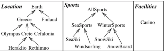
Assume that we want to build a Catalog of hotel Web pages and suppose that we want to provide access to these pages according to the Location of the hotels, the
Sports that are possible in these hotels, and the Facilities they offer. For doing
so, we can design a faceted taxonomy, i.e. a set of taxonomies, each describing the domain from a different aspect, or facet, like the one shown in Figure 1. Now each object (here Web page) can be indexed using a compound term, i.e., a set of terms from the different facets. For example, a hotel in Rethimno providing sea ski and wind-surfing sports can be indexed by assigning to it the compound term
{Rethimno, SeaSki, W indsurf ing}. We shall use the term materialized faceted taxonomy to refer to a faceted taxonomy accompanied by a set of object indices.
However, one can easily see that several compound terms over this faceted taxonomy are meaningless (or invalid), in the sense they cannot be applied to any object of the domain. For instance, we cannot do any winter sport in the
SeaSports WinterSports AllSports SnowBoard SeaSki Casino Greece Heraklio Rethimno Crete Finland Earth Olympus Sports Facilities Cefalonia Windsurfing SnowSki Location
Fig. 1. A faceted taxonomy for indexing hotel Web pages
Greek islands (Crete and Cefalonia) as they never have enough snow, and we cannot do any sea sport in Olympus because Olympus is a mountain. For the sake of this example, suppose that only in Cefalonia there exists a hotel that has a casino, and that this hotel also offers sea ski and wind-surfing sports. According to this assumption, the partition of compound terms to the set of
valid (meaningful) compound terms and invalid (meaningless) compound terms
is shown in Table 2 (found in Appendix A).
The availability of such a partition would be very useful during the construc-tion of a materialized faceted taxonomy. It could be exploited in the indexing process for preventing indexing errors, i.e. for allowing only meaningful com-pound terms to be assigned to objects. In particular, knowing this partition, it is possible to generate a ”complete” navigation tree, whose dynamically generated nodes correspond to all possible valid compound terms [19]. Such a navigation tree can aid the indexer to select the desired compound term for indexing, by browsing only the meaningful compound terms. This kind of ”quality control” or ”indexing aid” is especially important in cases where the indexing is done by many people who are not domain experts. For example, the indexing of Web pages in the Open Directory (which is used by Google and several other search engines) is done by more than 20.000 volunteer human editors (indexers). Apart from the indexer, the final user is also aided during his/her navigation and search by browsing only the meaningful compound terms.
However, even from this toy example, it is obvious that the definition of such a partition would be a formidably laborious task for the designer. Fortunately, the recently emerged Compound Term Composition Algebra (CTCA) [19] (which is recalled in Section 2.2) can significantly reduce the required effort. According to that approach the designer can use an algebraic expression to define the valid compound terms by declaring only a small set of valid or invalid compound terms from which other (valid or invalid) compound terms are then inferred. For instance, the partition shown in Table 2, can be defined using the expression:
e = (Location ªN Sports) ⊕PF acilities with the following P and N parameters:
N = {{Crete, W interSports}, {Cef alonia, W interSports}} P = {{Cef alonia, SeaSki, Casino},
In this paper we study the inverse problem, i.e. how we can derive an alge-braic expression e (like the above) that specifies exactly those compound terms that are extensionally valid (i.e. have non-empty interpretation) in an existing materialized faceted taxonomy. This problem, which we shall hereafter call
ex-pression mining or exex-pression extraction, has several applications. For instance,
it can be applied to materialized faceted taxonomies (which were not defined using the CTCA) in order to encode compactly and subsequently reuse the set of compound terms that are extensionally valid (e.g. the set of valid compound terms in Table 2). For example, suppose that we have in our disposal a very large medical file which stores medical incidents classified according to various aspects (like disease, symptoms, treatment, duration of treatment, patient’s age, genre, weight, smoking habits, patient’s profession, etc.), each one having a form of a hierarchy. In this scenario, expression mining can be used for extracting in a very compact form the set of all different combinations that have been recorded so far.
Moreover, it can be exploited for reorganizing single-hierarchical (non-faceted) materialized taxonomies (like the directories of Yahoo! or Google), so as to give them a clear faceted structure but without loosing the knowledge encoded in their taxonomy. Such a reorganization would certainly facilitate their manage-ment, extension, and reuse. Furthermore, it would allow the dynamic derivation of ”complete” and meaningful navigational trees for this kind of sources (as described in detail in [19]), which unlike the existing navigational trees of the single-hierarchical taxonomies, do not present the problem of missing terms or missing relationships (for more about this problem see [5]). For example, for reusing the taxonomy of the Google directory, we now have to copy its entire taxonomy which currently consists of more than 450.000 terms and whose RDF representation5 is a compressed file of 46 MBytes! According to our approach,
we only have to partition their terminologies to a set of facets, using languages like the one proposed in [17] (we will not elaborate this problem in this pa-per), and then use the algorithms presented in this paper for expression mining. One important remark that we have to mention here is that the closed world assumptions of the algebraic operations of the CTCA (described in [18]) lead us to a remarkably high ”compression ratio”. Apart from smaller storage space requirements, the resulted faceted taxonomy can be modified/customized in a more flexible and efficient manner. Furthermore, a semantically clear, faceted structure can aid the manual or automatic construction of the inter-taxonomy mappings [20], which are needed in order to build mediators or peer-to-peer sys-tems over this kind of sources [21]. Figure 2 illustrates graphically our problem and its context. Other applications of expression mining are presented in the concluding section.
Note that here ”mining” does not have the classical statistical nature, i.e. we are not trying to mine statistically justified associations or rules [7]. Instead, from an object base we are trying to mine the associations of the elements of
Complete, and Valid Navigational Trees D C B A process object indexing expression mining dynamically
Eg: ODP, Yahoo!
Materialized Taxonomy
missing terms and relationships
Materialized Faceted Taxonomy Faceted Taxonomy algebraic expression (A[+]B)[−](C[+]D) D C B A terms to facets partitioning object base object base
Fig. 2. The application context of expression mining
the schema (here of the terms of the faceted taxonomy) that capture informa-tion about the knowledge domain and were never expressed explicitly. Now, as the number of associations of this kind can be very big, we employ CTCA for encoding and representing them compactly.
The rest of this paper is organized as follows: Section 2 describes the required background and Section 3 states the problem. Section 4 describes straightforward methods for extracting an algebraic expression that specifies the valid compound terms of a materialized faceted taxonomy. Section 5 describes the method and the algorithms for finding the shortest, i.e. most compact and efficient expression. Additionally, it gives a demonstrating example. Finally, Section 6 concludes the paper and identifies issues for further research. A table of symbols is given in Appendix B.
2
Background
For self-containment, in the following two subsections, we briefly recall tax-onomies, faceted taxtax-onomies, compound taxtax-onomies, and the Compound Term Composition Algebra. For more information and examples please refer to [19, 18]. In subsection 2.3, we define materialized faceted taxonomies.
2.1 Taxonomies, Faceted Taxonomies, and Compound Taxonomies A taxonomy is a pair (T , ≤), where T is a terminology and ≤ is a reflexive and transitive relation over T , called subsumption.
A compound term over T is any subset of T . For example, the following sets of terms are compound terms over the taxonomy Sports of Figure 1: s1= {SeaSki, W indsurf ing}, s2 = {SeaSports, W interSports}, s3 = {Sports},
and s4 = ∅. We denote by P (T ) the set of all compound terms over T (i.e.
A compound terminology S over T is any set of compound terms that contains the compound term ∅.
The set of all compound terms over T can be ordered using an ordering relation that is derived from ≤. Specifically, the compound ordering over T is defined as follows: if s, s0 are compound terms over T , then s ¹ s0 iff ∀t0 ∈
s0 ∃t ∈ s such that t ≤ t0. That is, s ¹ s0 iff s contains a narrower term for every term of s0. In addition, s may contain terms not present in s0. Roughly,
s ¹ s0 means that s carries more specific indexing information than s0. Figure 3(a) shows the compound ordering over the compound terms of our previous example. Note that s1 ¹ s3, as s1 contains SeaSki which is a term narrower
than the unique term Sports of s3. On the other hand, s1 6¹ s2, as s1 does not
contain a term narrower than W interSports. Finally, s2 ¹ s3 and s3 ¹ ∅. In
fact, s ¹ ∅, for every compound term s.
{Sports} (b) (a) s2 {SeaSports, WinterSports} s1 s3 {SeaSports} {Sports} {Greece} {Greece,SeaSports} {Greece,Sports} {SeaSki, Windsurfing}
Fig. 3. Two examples of compound taxonomies
A compound taxonomy over T is a pair (S, ¹), where S is a compound termi-nology over T , and ¹ is the compound ordering over T restricted to S. Clearly, (P (T ), ¹) is a compound taxonomy over T .
The broader and the narrower compound terms of a compound term s are defined as follows: Br(s) = {s0∈ P (T ) | s ¹ s0} and Nr(s) = {s0 ∈ P (T ) | s0 ¹
s}. The broader and the narrower compound terms of a compound terminology S
are defined as follows: Br(S) = ∪{Br(s) | s ∈ S} and N r(S) = ∪{Nr(s) | s ∈ S}. Let {F1, ..., Fk} be a finite set of taxonomies, where Fi= (Ti, ≤i), and assume that the terminologies T1, ..., Tkare pairwise disjoint. Then, the pair F = (T , ≤ ), where T = ∪k
i=1Ti and ≤ = ∪ki=1 ≤i, is a taxonomy, which we shall call the
faceted taxonomy generated by {F1, ..., Fk}. We call the taxonomies F1, ..., Fkthe
facets of F.
Clearly, all definitions introduced so far apply also to faceted taxonomies. In particular, compound terms can be derived from a faceted taxonomy. For example, the set S = {{Greece}, {Sports}, {SeaSports}, {Greece, Sports},
{Greece, SeaSports}, ∅} is a compound terminology over the terminology T of
the faceted taxonomy shown in Figure 1. The set S together with the compound ordering of T (restricted to S) is a compound taxonomy over T . This compound taxonomy is shown in Figure 3.(b). For reasons of brevity, hereafter we shall omit the term ∅ from the compound terminologies of our examples and figures.
2.2 The Compound Term Composition Algebra
Here we present in brief the Compound Term Composition Algebra (CTCA), an algebra for specifying the valid compound terms of a faceted taxonomy (for further details see [19, 18]).
Let F = (T , ≤) be a faceted taxonomy generated by a set of facets {F1, ..., Fk}, where Fi= (Ti, ≤i). The basic compound terminology of a terminology Ti is de-fined as follows:
Ti= {{t} | t ∈ Ti} ∪ {∅}
Note that each basic compound terminology is a compound terminology over
T . The basic compound terminologies {T1, ..., Tk} are the initial operands of the algebraic operations of CTCA.
The algebra includes four operations which allow combining terms from dif-ferent facets, but also terms from the same facet. Two auxiliary product opera-tions, one n-ary (⊕) and one unary (⊕), are defined to generate all combinations∗
of terms from different facets and from one facet, respectively. Since not all term combinations are valid, more general operations are defined that include
positive or negative modifiers, which are sets of known valid or known invalid
compound terms. The unmodified product and self-product operations turn out to be special cases with the modifiers at certain extreme values. Specifically, the four basic operations of the algebra are: plus-product (⊕P), minus-product (ªN), plus-self-product (
∗
⊕P), and minus-self-product ( ∗
ªN), where P denotes a set of valid compound terms and N denotes a set of invalid compound terms. The definition of each operation is given in Table 1.
Operation e Se product S1⊕ ... ⊕ Sn { s1∪ ... ∪ sn| si∈ Si} plus-product ⊕P(S1, ...Sn) S1∪ ... ∪ Sn ∪ Br(P ) minus-product ªN(S1, ...Sn) S1⊕ ... ⊕ Sn− N r(N ) self-product ⊕ (T∗ i) P (Ti) plus-self-product ⊕∗P (Ti) Ti∪ Br(P ) minus-self-product ª∗N(Ti) ∗ ⊕ (Ti) − N r(N )
Table 1. The operations of the Compound Term Composition Algebra
For example, consider the compound terminologies S = {{Greece}, {Islands}} and S0= {{Sports}, {SeaSports}}. The compound taxonomy corresponding to
S ⊕ S0 is shown in Figure 4, and consists of 8 terms.
Now consider the compound terminologies S and S0 shown in the left part of Figure 5, and suppose that we want to define a compound terminology that does not contain the compound terms {Islands, W interSports} and {Islands,
SnowSki}, because they are invalid. For this purpose instead of using a product,
{Sports} {SeaSports} S S’ {SeaSports} {Sports} S S’ {Islands} {Islands,Sports} {Greece,Sports} {Greece} {Greece} {Islands} {Greece,SeaSports} {Islands,SeaSports}
Fig. 4. An example of a product ⊕ operation
Specifically, we can use a plus-product, ⊕P(S, S0), where P = {{Islands,
Seasports}, {Greece, SnowSki}}. The compound taxonomy defined by this
op-eration is shown in the right part of Figure 5. In this figure we enclose in squares the elements of P . We see that the compound terminology ⊕P(S, S0) contains the compound term s = {Greece, Sports}, as s ∈ Br({Islands, SeaSports}). How-ever, it does not contain the compound terms {Islands, W interSports} and
{Islands, SnowSki} as they do not belong to S ∪ S0∪ Br(P ) (see the definition of plus-product in Table 1). P {Greece, SnowSki}} ={{Islands,SeaSports}, P(S,S’) {Greece,Sports} {Greece} {Sports} {WinterSports} {Greece,SeaSports} {Islands,Sports} {Greece,WinterSports} {Greece,SnowSki} {Islands,SeaSports} {SeaSports} {Islands} {SnowSki} {WinterSports} {SeaSports} {SnowSki} {Sports} S’ {Greece} {Islands} S
Fig. 5. An example of a plus-product, ⊕P, operation
Alternatively, we can obtain the compound taxonomy shown at the right part of Figure 5 by using a minus-product operation, i.e. ªN(S, S0), with N =
{{Islands, W interSports}}. The result does not contain the compound terms {Islands, W interSports} and {Islands, SnowSki}, as they are elements of N r(N ) (see the definition of minus-product in Table 1).
An expression e over F is defined according to the following grammar (i = 1, ..., k): e ::= ⊕P(e, ..., e) | ªN (e, ..., e) | ∗ ⊕P Ti | ∗ ªN Ti| Ti,
where the parameters P and N denote sets of valid and invalid compound terms, respectively. The outcome of the evaluation of an expression e is denoted by Se, and is called the compound terminology of e. In addition, (Se, ¹) is called the compound taxonomy of e. According to our semantics, all compound terms in Seare valid, and the rest in P (T ) − Seare invalid [18].
To proceed we need to distinguish what we shall call genuine compound terms. Intuitively, a genuine compound term combines non-empty compound terms from more than one compound terminologies. Specifically, the set of genuine
compound terms over a set of compound terminologies S1, ..., Sn is defined as follows:
GS1,...,Sn= S1⊕ ... ⊕ Sn− ∪ n i=1Si
For example, if S1= {{Greece}, {Islands}}, S2= {{Sports}, {W interSports}},
and S3= {{P ensions}, {Hotels}} then {Greece, W interSports, Hotels} ∈ GS1,S2,S3, {W interSports, Hotels} ∈ GS1,S2,S3, but {Hotels} 6∈ GS1,S2,S3.
Additionally, the set of genuine compound terms over a basic compound ter-minology Ti, i = 1, ..., k, is defined as follows: GTi =
∗
⊕ (Ti) − Ti.
The sets of genuine compound terms are used to define a well-formed alge-braic expression.
An expression e is well-formed iff:
(i) each basic compound terminology Ti appears at most once in e,
(ii) each parameter P that appears in e, is a subset of the associated set of genuine compound terms, e.g. if e = ⊕P(e1, e2) then it should be P ⊆ GSe1,Se2, and
(iii) each parameter N that appears in e, is a subset of the associated set of genuine compound terms, e.g. if e =ª∗N (Ti) then it should be N ⊆ GTi.
For example, the expression6 (T
1 ⊕P T2) ªN T1 is not well-formed, as T1
appears twice in the expression. Constraints (i), (ii), and (iii) ensure that the evaluation of an expression is monotonic, meaning that the valid and invalid com-pound terms of an expression e increase as the length of e increases. For example, if we omit constraint (i) then an invalid compound term according to an expres-sion T1⊕PT2could be valid according to a larger expression (T1⊕PT2) ⊕P0T1. If we omit constraint (ii) then an invalid compound term according to an expres-sion T1⊕P1T2could be valid according to a larger expression (T1⊕P1T2) ⊕P2T3.
Additionally, if we omit constraint (iii) then a valid compound term accord-ing to an expression T1⊕P T2 could be invalid according to a larger expression
(T1⊕P T2) ªNT3.
In the rest of the paper, we consider only well-formed expressions. In [19], we presented the algorithm IsV alid(e, s) that takes as input a (well-formed) expression e and a compound term s, and checks whether s ∈ Se. This algorithm has polynomial time complexity, specifically O(|T |2∗ |s| ∗ |P ∪ N |), where P
denotes the union of all P parameters of e, and N denotes the union of all N parameters of e.
Additionally, [18] defines the semantics of CTCA and shows why we cannot use Description Logics [8] to represent the compound term composition algebra. At last we should mention that a system that supports the design of faceted tax-onomies and the interactive formulation of CTCA expressions has already been
implemented by VTT and Helsinki University of Technology (HUT) under the name FASTAXON [3]. The system is currently under experimental evaluation. 2.3 Materialized Faceted Taxonomies
Let Obj denote the set of all objects of our domain, e.g. the set of all hotel Web pages. An interpretation of a set of terms T over Obj is any (total) function
I : T → P (Obj).
A materialized faceted taxonomy M is a pair (F, I), where F= (T , ≤) is a faceted taxonomy, and I is an interpretation of T .
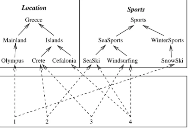
An example of a materialized faceted taxonomy is given in Figure 6, where the objects are denoted by natural numbers. This will be the running example of our paper. 1 SeaSki Windsurfing SeaSports WinterSports SnowSki 3 4 2 Sports Sports Mainland Olympus Crete Islands Greece Cefalonia Location
Fig. 6. A materialized faceted taxonomy
Apart from browsing, we can also query a materialized faceted taxonomy. A simple query language is introduced next. A query over T is any string derived by the following grammar: q ::= t | q ∧ q0| q ∨ q0 | q ∧ ¬q0 | (q) | ², where t is a term of T . Now let QT denote the set of all queries over T . Any interpretation
I of T can be extended to an interpretation ˆI of QT as follows: ˆI(t) = I(t), ˆ
I(q ∧ q0) = ˆI(q) ∩ ˆI(q0), ˆI(q ∨ q0) = ˆI(q) ∪ ˆI(q0), ˆI(q ∧ ¬q0) = ˆI(q) \ ˆI(q0). One can easily see that a compound term {t1, ..., tk} actually corresponds to a conjunction
t1∧ ... ∧ tk. However, in order for answers to make sense, the interpretation used for answering queries must respect the structure of the faceted taxonomy in the following intuitive sense: if t ≤ t0 then I(t) ⊆ I(t0). The notion of model, introduced next, captures well-behaved interpretations. An interpretation I is a
model of a taxonomy (T , ≤) if for all t, t0 in T , if t ≤ t0 then I(t) ⊆ I(t0). Given an interpretation I of T , the model of (T , ≤) generated by I, denoted ¯
I, is given by: ¯I(t) = ∪{I(t0) | t0 ≤ t}. Now the answer of a query q is the set of objects ˆ¯I(q). For instance, in our running example we have ˆ¯I(Islands) = {2, 3, 4}, ˆ¯I({Crete, SeaSki}) = {2}, and ˆ¯I({SeaSki, W indsurf ing}) = {4}.
3
Problem Statement
The set of valid compound terms of a materialized faceted taxonomy M = (F, I) is defined as:
V (M ) = {s ∈ P (T ) | ˆ¯I(s) 6= ∅}
where ¯I is the model of (T , ≤) generated by I.7
The following table indicates the valid compound terms of the materialized faceted taxonomy shown in Figure 6, that contain exactly one term from each facet.
Greece Mainl. Olymp. Islands Crete Cefal.
Sports √ √ √ √ √ √ SeaSports √ √ √ √ SeaSki √ √ √ √ Windsurf. √ √ √ √ WinterSp. √ √ √ SnowSki √ √ √
Our initial problem of expression mining is formulated as follows: Problem 1: Given a materialized faceted taxonomy M = (F, I), find
an expression e over F such that Se= V (M ).
Let us define the size of an expression e as follows: size(e) = |P ∪ N |, where P denotes the union of all P parameters of e, and N denotes the union of all N parameters of e. Among the expressions e that satisfy Se = V (M ), we are more interested in finding the shortest expression. This is because, in addition to smaller space requirements, the time needed for checking compound term validity according to the mined expression e is reduced8. Reducing the
time needed for checking compound term validity, improves the performance of several on-line tasks associated with knowledge reuse. Indeed, as it was shown in [19], the algorithm IsV alid(e, s) is called during the dynamic construction of the navigation tree that guides the indexer and the final user through his/her (valid) compound term selection. Though, shortest expression mining is a costly operation, it is not a routine task. Therefore, we consider that reducing the size of the mined expression is more important than reducing the time needed for its extraction. In particular, we are interested in the following problem:
Problem 2: Given a materialized faceted taxonomy M = (F, I), find
the shortest expression e over F such that Se= V (M ).
One important remark is that solving the above problem allow us to solve also the following:
7 As all single terms of a faceted taxonomy are meaningful, we assume that V (M )
contains all singleton compound terms.
8 Recall that the time complexity of Alg. IsV alid(e, s) [19] is proportional to size(e) =
Problem 3: Given an expression e0, find the shortest expression e such
that Se= Se0.
One can easily see that the same algorithms can be used for solving both Problem 2 and Problem 3. The only difference is that, in the second problem we have to consider that V (M ) is the set Se0. Note that this kind of ”optimization” could be very useful even during the design process, i.e. a designer can use sev-eral times the above ”optimizer” during the process of formulating an algebraic expression.
For simplicity, in this paper we do not consider self-product operations. Their inclusion is a trivial extension of the presented methods. Therefore, from V (M ) we consider only the compound terms that contain at most one term from each facet.
4
Mining an Expression
One straightforward method to solve Problem 1 is to find an expression e with only one plus-product operation over the basic compound terminologies
T1, ..., Tk, i.e. an expression of the form: e = ⊕P(T1, ..., Tk).
We can compute the parameter P of this operation in two steps: 1. P0 := V (M ) ∩ G
T1,...,Tk 2. P := minimal(P0).
The first step computes all valid compound terms that (a) contain at most one term from each facet, and (b) do not belong to basic compound terminologies, i.e. are not singletons. One can easily see that S⊕P 0(T1,...,Tk) = V (M ). The second step is optional and aims at reducing the size of the mined expression. Specifically, it eliminates the redundant compound terms of the parameter P0, i.e. those compound terms that are not minimal (w.r.t. ¹). This is because, it holds:
⊕P0(T1, ..., Tk) = ⊕minimal(P0)(T1, ..., Tk)
Thus, if P contains the minimal elements of P0, then it is evident that again it holds S⊕P(T1,...,Tk) = V (M ). By applying the above two-step algorithm to our current example we get that:
P = {{Olympus, SnowSki}, {Crete, SeaSki}, {Crete, W indsurf ing}, {Cef alonia, SeaSki}, {Cef alonia, W indsurf ing}}
Analogously, we can find an expression e with only one minus-product oper-ation over the basic compound terminologies T1, ..., Tk, i.e. an expression of the form: e = ªN(T1, ..., Tk).
1. N0 := G
T1,...,Tk\ V (M ) 2. N := maximal(N0)
The first step computes all invalid compound terms that contain at most one term from each facet. One can easily see that SªN 0(T1,...,Tk)= V (M ). Again, the second step is optional and aims at reducing the size of the mined expression. Specifically, it eliminates the redundant compound terms, i.e. compound terms that are not maximal (w.r.t. ¹). This is because, it holds:
ªN0(T1, ..., Tk) = ªmaximal(N0)(T1, ..., Tk)
Thus, if N contains the maximal elements of N0, then it is evident that again it holds SªN(T1,...,Tk) = V (M ). By applying the above two-step algorithm to our current example we get that:
N = {{M ainland, SeaSports}, {Islands, W interSports}}
Notice that here the size of the minus-product expression is smaller than that of the plus-product expression (the parameter N contains only 2 compound terms, while P contains 5).
5
Mining the Shortest Expression
Let us now turn our attention to Problem 2, i.e. on finding the shortest expression
e over a given a materialized faceted taxonomy M = (F, I), such that Se =
V (M ).
At first notice that since our running example has only two facets, the shortest expression is either a plus-product or a minus-product operation. However, in the general case where we have several facets, finding the shortest expression is more complicated because there are several forms that an expression can have.
Below we present the algorithm F indShortestExpression( F, V ) (Alg. 51) which takes as input a faceted taxonomy F and a set of compound terms V , and returns the shortest expression e over F such that Se = V . It is an ex-haustive algorithm, in the sense that it investigates all forms that an expression over F may have. We use the term expression form to refer to an algebraic ex-pression whose P and N parameters are undefined (unspecified). Note that an expression form can be represented as a parse tree. Specifically, the procedure
P arseT rees({F1, ..., Fn}) (which is described in detail in subsection 5.1) takes as input a set of facets {F1, ..., Fn} and returns all possible parse trees of the expressions over {F1, ..., Fn}.
Now the procedure Specif yP arams(e, V ) (which is described in detail in subsection 5.2) takes as input a parse tree e and a set of compound terms V ⊆
P (T ), and specifies the parameters P and N of e such that Se= V .
The procedure GetSize(e) takes as input an expression e and returns the
size of e, i.e. |P ∪ N |.9
9 We could also employ a more refined measure for the size of an expression, namely the
exact number of terms that appear in the parameter sets, i.e. size(e) =Ps∈P∪N|s|
Finally, the algorithm F indShortestExpression(F,V ) returns the shortest expression e such that Se= V . Summarizing, F indShortestExpression(F,V (M )) returns the solution to Problem 2.
Algorithm 51 F indShortestExpression(F, V )
Input: A faceted taxonomy F generated by {F1, ..., Fk}, and a set of compound terms
V
Output: The shorthest expression e such that Se= V
minSize := MAXINT; shortestExpr := ””;
For each e in ParseTrees({F1, ..., Fk}) do
e0 := SpecifyParams(e, V );
size := GetSize(e0);
If size < minSize then
minSize := size; shortestExpr := e0;
EndIf EndFor
return (shortestExpr)
5.1 Deriving all Possible Parse Trees
In this subsection, we describe how we can compute the parse trees of all possi-ble expressions over a set of facets {F1, ..., Fn}. Recall that the parse tree of an expression is a tree structure that describes a derivation of the expression ac-cording to the rules of the grammar. A depth-first-search traversal of the parse tree of an expression e can be used to obtain the prefix form of the expres-sion e. In our case, the terminal (leaf) nodes of a parse tree are always facet names10. Additionally, the internal nodes of a parse tree are named ”+” or ”-”,
corresponding to a plus-product (⊕P) or a minus-product (ªN) operation, re-spectively. For example, Figure 7(c) displays all different parse trees for the set of facets {A, B, C}. Note that every facet appears just once in a parse tree, as we consider only well-formed expressions.
Algorithm P arseT rees({F1, ..., Fn}) (Alg. 52) takes as input a set of facet names {F1, ..., Fn} and returns all possible parse trees for {F1, ..., Fn}. We will first exemplify the algorithm and its reasoning through a small example.
Consider the facets {A, B, C} of our current example. We will use a recursive method for computing the parse trees for {A, B, C}. At first, we find the parse trees for {A}. Clearly, there is only one parse tree for {A}, and it consists of a single node with name A (see Figure 7(a)). Subsequently, we find the parse trees
10Specifically, a terminal node with name F
icorresponds to the basic compound
− + − − − − A C B + − + − − − − + A B C + − + + A B C + + A C B + − + + + − + A C B A C B ParseTrees({A,B,C}) ParseTrees({A,B}) ParseTrees({A}) (c) (b) (a) A B A A B A C B A B C A B C A B C A B C − A C B A C B A C B tr0 tr3 tr4 tr5 tr6 tr7 tr8 tr9 tr1 tr2 n1 n2 n3
Fig. 7. All possible parse trees for {A}, {A, B}, and {A, B, C}
of {A, B}. There are two ways for extending the parse tree for {A} with the new facet B: (i) by creating a ”+” node with children A and B, and (ii) by creating a ”-” node with children A and B. Thus, we can create two parse trees for {A, B}, named tr1 and tr2 (see Figure 7(b)). In other words, P arseT rees({A, B}) = {tr1, tr2}, where the parse tree tr1 corresponds to ⊕(A, B), and the parse tree tr2 corresponds to ª(A, B).
Now, we can find the parse trees of {A, B, C}, by extending each node of each parse tree in P arseT rees({A, B}) with the new facet C. For doing so, initially we visit the parse tree tr1. At first we visit the internal node n1 of tr1 and we
extend it in three different ways (all other nodes of tr1 remain the same):
1. by adding C to the children of n1. Now n1 corresponds to the operation ⊕(A, B, C), and this extension results to the parse tree tr3.
2. by creating a new ”+” node with children the nodes n1 and C. The new
node corresponds to ⊕(⊕(A, B), C), and this extension results to the parse tree tr4.
3. by creating a new ”-” node with children the nodes n1and C. The new node
corresponds to ª(⊕(A, B), C), and this extension results to the parse tree
tr5.
Now, we visit the terminal node n2 of tr1and we extend it in two different ways:
1. by creating a new ”+” node with children the nodes n2 and C. The new
node corresponds to the operation ⊕(A, C), and this extension results to the parse tree tr6.
2. by creating a new ”-” node with children the nodes n2and C. The new node
corresponds to the operation ª(A, C), and this extension results to the parse tree tr7.
Finally, we visit the terminal node n3 of tr1 and we extend it in two different
ways, similarly to node n2. These extensions result to the parse trees tr8 and tr9.
After finishing with tr1, we visit tr2and we extend each node of tr2with the
new facet C, similarly to tr1. Figure 7(c) gives all the parse trees for {A, B, C}.
Generally, the above process is repeated recursively until all the facets of a faceted taxonomy have been considered.
Algorithm 52 P arseT rees({F1, ..., Fn})
Input: A set {F1, ..., Fn} of facet names
Ouptut: All possible parse trees for {F1, ..., Fn}
(1) If n = 1 then return({CreateNode(F1)});
(2) allP trees := {};
(3) For each ptree ∈ ParseTrees({F1, ..., Fn−1}) do
(4) allP trees := allP trees∪ ExtendedTrees(ptree, ptree, Fn);
(5) return(allP trees)
Below we will describe in detail the algorithms needed for deriving all possible parse trees. Given a node n we shall use n.Parent to refer to the parent of n, and Children(n) to the children of node n. We shall also use the following auxiliary routines: CreateNode(nm) a function that creates and returns a new node with name nm, and IsTerminal(n) a function that returns true if n is a terminal node, and false otherwise.
Let us now describe in detail the algorithm P arseT rees( {F1, ..., Fn}) (Alg. 52). The procedure P arseT rees({F1, ..., Fn}) calls P arseT rees({F1, ..., Fn−1}). Then, for each parse tree ptree returned by P arseT rees({F1, ..., Fn−1}), it issues the call ExtendedT rees(ptree, ptree, Fn).
Let us now see what ExtendedT rees(ptree, extN ode, F n) (Alg. 53) does. The procedure takes as input a parse tree ptree, a node extN ode11of the ptree, and
a facet name F n. It returns a set of parse trees that correspond to the extension of ptree with the new facet name F n, at the node extN ode. Now the way the extension is performed depends on the kind of the node extN ode (i.e. terminal or internal). Specifically, there are two cases:
C1: extN ode is a terminal node (say Fi).
In this case the lines (3)-(6) produce two copies of the ptree (called ptree+
and ptree−, respectively), and call the routine ExtendT reeN ode that does that actual extension. After the execution of these lines,
ptree+corresponds to the extension ⊕(Fi, Fn), and
ptree− corresponds to the extension ª(Fi, Fn).
The exact algorithm for ExtendT reeN ode is presented below in this section (Alg. 54). The function T reeCopy(ptree) takes as input a parse tree ptree
11It is named extN ode, because the operation corresponding to that node will be
and returns a copy, say ptree copy, of ptree. Notice that according to line (1), ptree keeps a pointer ExtN ode to the node extN ode. After the call of
T reeCopy(ptree), ptree copy.ExtN ode points to the copy of the extN ode in
the ptree copy.
C2: extN ode is an internal node (i.e. either ”+” or ”-”).
This means that extN ode corresponds to either a ⊕(e1, ..., ei) or a ª(e1, ..., ei) operation. Below we shall write ¯(e1, ..., ei) to denote any of the above two operations.
In this case the routine ExtendT reeN ode is called three times (lines (10)-(14)): These calls produce three copies of ptree, namely ptreein, ptree+, and ptree−, where:
ptreeincorresponds to the extension ¯(e1, ..., ei, Tn),
ptree+corresponds to the extension ⊕(¯(e1, ..., ei), Tn), and
ptree− corresponds to the extension ª(¯(e1, ..., ei), Tn).
At last, the routine ExtendedT rees(ptree, extN ode, F n) calls itself
(ExtendedT rees(ptree, childN ode, F n)), for each child childN ode of the node extN ode.
Algorithm 53 ExtendedT rees(ptree, extN ode, F n)
Input: a parse tree ptree, a node extN ode of ptree, and a facet name F n
Output: a set of parse trees that correspond to the extension of ptree with the new
facet name F n, at the node extN ode (1) ptree.ExtN ode := extN ode; (2) If IsTerminal(extN ode) then (3) ptree+ := TreeCopy(ptree);
(4) ExtendTreeNode(ptree+.ExtN ode, ”+”, F n);
(5) ptree−:= TreeCopy(ptree);
(6) ExtendTreeNode(ptree−.ExtN ode, ”-”, F n);
(7) return({ptree+, ptree−})
(8) Else // extNode is an internal node (9) ptree+ := TreeCopy(ptree);
(10) ExtendTreeNode(ptree+.ExtN ode, ”+”, F n);
(11) ptree−:= TreeCopy(ptree);
(12) ExtendTreeNode(ptree−.ExtN ode, ”-”, F n);
(13) ptreein := TreeCopy(ptree);
(14) ExtendTreeNode(ptreein.ExtN ode, ”in”, F n);
(15) extendedT rees :={ptreein, ptree+, ptree−};
(16) For each childN ode ∈ Children(extN ode) do (17) extendedT rees := extendedT rees ∪
ExtendedTrees(ptree, childN ode, F n) ; (18) return(extendedT rees)
Algorithm 54 ExtendT reeN ode(extN ode, f lag, F n)
Input: a node extN ode of a parse tree, a flag f lag that denotes the type of the extension
with the new facet name F n, and a facet name F n
Output: the parse tree extended with F n at the extN ode, according to f lag
(1) F nN ode :=CreateNode(F n) ; (2) If f lag =”in” then
(3) F nN ode.Parent := extN ode ;
(4) If f lag=”+” or f lag=”-” then
(5) newOpN ode :=CreateNode(f lag);
(6) F nN ode.Parent := newOpN ode ;
(7) InsertBetween(extN ode.Parent, extN ode, newOpN ode); (8) End if
Notice that Alg. 54 uses the function InsertBetween(nU p, nDown, new). This function inserts the node new between the nodes nU p and nDown. This means that after this call, it holds nDown.Parent = new and new.Parent =
nU p. Clearly, if nU p is nil then new becomes root node.
As an example, Figure 7(b) shows the output of P arseT rees({A, B}). Figure 7(c) shows the output of P arseT rees({A, B, C}). The first row of the parse trees in Figure 7(c) corresponds to the parse trees returned by ExtendedT rees(tr1, tr1, C) and the second row corresponds to the parse trees returned by ExtendedT rees(tr2,
tr2, C).
As a final comment note that some parse trees returned by P arseT rees({F1, ..., Fk}) can been eliminated before Specif yP arams(e, V ) is called by algorithm
F indShortestExpression(F, V ) (Alg. 51), for setting up the parameters. This
is because, these parse trees cannot yield to the shortest expression. For example, consider the parse trees tr3 and tr4 of Figure 7(c). The parse tree tr4 can be elim-inated, because tr4 can never yield to an expression with size less than that of tr3. Actually, more than half of the parse trees returned by P arseT rees({F1, ..., Fk}) are redundant, and thus can be ignored. For example, from the 162 parse trees returned by P arseT rees({A, B, C, D}) only 64 are good candidates for yielding the shortest expression.
5.2 Specifying the Parameters
This section describes the algorithm Specif yP arams(e, V ) (Alg. 55), i.e. an algorithm that takes as input the parse tree of an expression e (with undefined
P and N parameters) and a set of compound terms V ⊆ P (T ), and returns
the same parse tree that is now enriched with P and N parameters that satisfy the condition Se= V . Of course, this is possible only if Br(V ) = V (note that
Algorithm 55 Specif yP arams(e, V )
Input: The parse tree of an expression e, and a set of compound terms V ⊆ P (T ) Output: The parse tree of e enriched with P and N parameters, such that Se= V
(1) case(e) { (2) ⊕P(e1, ..., en): For i := 1, ..., n do (3) ei := SpecifyParams(ei, V ) ; (4) P0:= G Se1,...,Sen∩ V ; (5) e.P := minimal(P0) ; (6) return(e) (7) ªN(e1, ..., en): For i := 1, ..., n do (8) ei := SpecifyParams(ei, V ) ; (9) N0:= G Se1,...,Sen\ V ; (10) e.N := maximal(N0) ; (11) return(e) (12) Ti: return(e) (13)}
Suppose that the current node is an internal node that corresponds to a plus-product operation ⊕P(e1, ..., en). For setting the parameter P of this operation we must first define the parameters of all subexpressions ei, for all i = 1, ..., n. Therefore, the procedure Specif yP arams(ei, V ) is called recursively, for all i = 1, ..., n. Subsequently, the statement P0:= G
Se1,...,Sen∩ V computes and stores in P0 those elements of V that also belong to G
Se1,...,Sen (recall constraint (ii) of a well-formed expression). Finally, P is set equal to the minimal compound terms of P0 (for the reasons described in Section 4).
Now suppose that the current node is an internal node that corresponds to a minus-product operation ªN(e1, ..., en). Again, before defining N we have to de-fine the parameters of all subexpressions ei, for all i = 1, ..., n. So, the procedure
Specif yP arams(ei, V ) is called recursively, for all i = 1, ..., n. Subsequently, the statement N0:= G
Se1,...,Sen \ V computes and stores in N0 those elements of
GSe1,...,Sen that are invalid, i.e. not in V (recall constraint (iii) of a well-formed expression). Finally, N is set equal to the maximal compound terms of N0 (for the reasons described in Section 4).
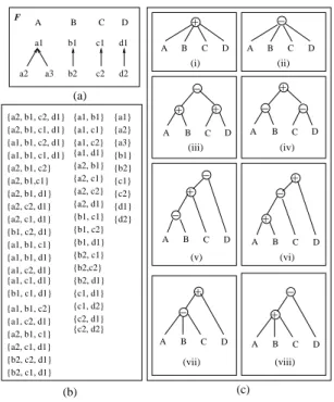
For example, consider the four-faceted taxonomy F shown in Figure 8(a), and suppose that V is the set of compound terms shown in Figure 8(b). Below we give the trace of execution of Specif yP arams(e, V ) for the expression e =
⊕P(A, ªN(B, C, D)):
call Specif yP arams(⊕P(A, ªN(B, C, D)), V ) call Specif yP arams(ªN(B, C, D), V )
return // N is set equal to {{b2, d2}} return // P is set equal to {{a2, b1, c2, d1}}
So the parameters of the resulting expression e are the following:
P = {{a2, b1, c2, d1}} N = {{b2, d2}}
5.3 An Example of Shortest Expression Mining
Let us now apply the above algorithms to the four-faceted taxonomy shown in Figure 8(a). The set of all compound terms that consist of at most one term from each facet are (|A| + 1) ∗ (|B| + 1) ∗ (|C| + 1) ∗ (|D| + 1) = 108. Now let us suppose that the set of valid compound terms V (M ) consists of the 48 compound terms listed in Figure 8(b). For simplification, in that figure we do not show the interpretation I, but directly the set V (M ).
(c) c2 c1 C b2 b1 B a3 a2 a1 A {b1, c1, d1} {a1, b1, c2} {a1, c2, d1} {a2, b1, c1} {a2, c1, d1} {b2, c2, d1} {b2, c1, d1} {a2, b1, c2, d1} {a1, b1} {a1, c1} {a1, c2} {a1, d1} {a2, b1} {a2, c1} {a2, c2} {a2, d1} {b1, c1} {b1, c2} {b1, d1} {b2, c1} {a1} {a3} {a2, b1, c1, d1} {a1, b1, c2, d1} {a1, b1, c1, d1} {a2} {b1} {b2} {c1} {c2} {d1} {d2} {c1, d2} {c1, d1} {b2,c2} {b2, d1} {c2, d1} {c2, d2} {a2, b1, d1} {a2, c2, d1} {a2, b1,c1} {a2, b1, c2} {a2, c1, d1} {b1, c2, d1} {a1, b1, c1} {a1, b1, d1} {a1, c2, d1} {a1, c1, d1} (b) + A B C D + + − A B C D − + − A B C D − + A B C D − A B C D − + − A B C D + − + A B C D + − A B C D (ii) (iv) (vi) (viii) d1 d2 D F (a) (i) (iii) (v) (vii)
Fig. 8. An example of expression mining
The algorithm F indShortestExpression(F, V (M )) calls the procedure
P arseT rees({A, B, C, D}), to get the parse trees of all possible expressions
over the facets {A, B, C, D} (Figure 8(c) sketches some indicative parse trees). Then, for each parse tree e in the output, it calls the procedure Specif yP
a-rams(e, V (M )), which assigns particular values to the parameters P and N of e
such that Se= V (M ). The sizes of all derived expressions are compared to get the shortest expression, which is the following:
P = {{a2, b1, c2, d1}} N = {{b2, d2}}
Notice that the size of |P ∪ N | is only 2! Even from this toy example it is evident that the expressions of the Compound Term Composition Algebra can indeed encode very compactly the knowledge of materialized taxonomies. As we have already mentioned, this is due to the closed world assumptions of the algebraic operations.
6
Conclusion
Mining commonly seeks for statistically justified associations or rules. In this paper we deal with a different kind of mining. Specifically, we show how from an object base we can mine the associations of the elements of the schema (here of the terms of a faceted taxonomy) that capture information about the knowledge domain and were never expressed explicitly. Now, as the number of associations of this kind can be very big, we employ the Compound Term Composition Algebra (CTCA) for encoding and representing these associations compactly.
Specifically, we confine ourselves to the case of materialized faceted tax-onomies (for more about faceted classification see [16, 9, 22, 11, 15]). Materialized faceted taxonomies are employed in several different domains, including Libraries [12], Software Repositories [13, 14], Web catalogs and many others. Current in-terest in faceted taxonomies is also indicated by several ongoing projects like FATKS12, FACET13, FLAMENGO14, and the emergence of XFML [1]
(Core-eXchangeable Faceted Metadata Language) that aims at applying the faceted classification paradigm on the Web.
In this paper we showed how we can find algebraic expressions of CTCA that specify exactly those compound terms that are extensionally valid (i.e. have non-empty interpretation) in a materialized faceted taxonomy. The size of the resulting expressions is remarkably low. In particular, we gave two straight-forward methods for extracting a plus-product and a minus-product expression (possibly, none the shortest), and an exhaustive algorithm for finding the short-est expression. The complexity of the latter is of course exponential with respect to the number of facets. This does not reduce the benefits of our approach, as the number of facets cannot practically be very big (we haven’t seen so far any faceted taxonomy with more than 10 facets), and expression mining is a rare off-line task. As explained in the paper, the time for checking compound term validity is proportional to expression size. Thus, we considered that slow runs of shortest expression mining can be tolerated in order to minimize the size of the mined expression and provide efficiency for later on-line tasks, such as object indexing and navigation.
12http://www.ucl.ac.uk/fatks/database.htm
13http://www.glam.ac.uk/soc/research/hypermedia/facet proj/index.php 14http://bailando.sims.berkeley.edu/flamenco.html
Expression mining can be exploited for encoding compactly the set of valid compound terms of materialized faceted taxonomies. This can significantly aid their exchange and reuse. It also worths mentioning here that the recently emerged XFML+CAMEL [2] (Compound term composition
Algebraically-M otivated Expression Language) allows publishing and exchanging faceted
tax-onomies and CTCA expressions using an XML format.
Expression mining also allows the reorganization of single-hierarchical ma-terialized taxonomies (such as Yahoo! and ODP), so as to give them a faceted structure without missing the knowledge encoded in their pre-coordinated terms. Such a reorganization would certainly facilitate their management, extension, and reuse. Furthermore, it would allow the dynamic derivation of ”complete” and valid navigational trees for this kind of sources [19].
Expression mining can also be exploited in language engineering. WordNet [6] is a lexical ontology where terms are grouped into equivalence classes, called
synsets. Each synset is assigned to a lexical category i.e. noun, verb, adverb, adjective, and synsets are linked by hypernymy/hyponymy, and antonymy
rela-tions. Clearly, by ignoring the antonymy relation, the rest can be seen as a faceted taxonomy with the following facets: noun, verb, adverb, and adjective. This faceted taxonomy plus any collection of indexed subphrases from a corpus of documents is actually a materialized faceted taxonomy that contains informa-tion about the concurrence of words (e.g. which adjectives are applied to which nouns). This kind of knowledge might be quite useful, as it can be exploited in several applications, e.g. for building a recommender system in a word processor (e.g. in MS Word), an automatic cross-language translator, or an information retrieval system (e.g. see [10]). Notice that in this scenario, the number of valid combinations of words would be so big, that storing them explicitly would be quite problematic. So, this scenario also indicates the need for expression mining, in order to extract and represent compactly the valid combinations of words.
Another application of expression is query answering optimization. Suppose a materialized faceted taxonomy that stores a very large number of objects at which users can pose conjunctive queries (i.e. compound terms) in order to find the objects of interest. The availability of the set of valid compound terms would allow realizing efficiently whether a query has an empty or a non-empty answer. In this way, we can avoid performing wasteful computations for queries whose answer will be eventually empty.
Issues for further research include measuring the exact time/space complex-ity of expression mining, designing optimal algorithms for shortest expression mining, and investigating whether it worths employing additional indexing data structures (e.g. labelling schemes like those mentioned in [4]) for further speed-up.
References
1. “XFML: eXchangeable Faceted Metadata Language”. http://www.xfml.org. 2. “XFML+CAMEL:Compound term composition Algebraically-Motivated
3. “FASTAXON: A system for FAST (and Faceted) TAXONomy design.”, 2004. To be published as an open source project in http://opensource.erve.vtt.fi/fastaxon. 4. Vassilis Christophides, Dimitris Plexousakis, Michel Scholl, and Sotirios
Tourtou-nis. On Labeling Schemes for the Semantic Web. In Proceedings of WWW’2003, pages 544–555, Budapest, Hungary, May 2003.
5. Peter Clark, John Thompson, Heather Holmback, and Lisbeth Duncan. “Exploit-ing a Thesaurus-based Semantic Net for Knowledge-based Search”. In Proceed“Exploit-ings
of 12th Conf. on Innovative Applications of AI (AAAI/IAAI’00), pages 988–995,
2000.
6. Princeton University Cognitive Science Laboratory. “WordNet: A Lexical Database for the English Language”. (http://www.cogsci.princeton.edu/ wn).
7. Padhraic Smyth David J. Hand, Heikki Mannila. Principles of Data Mining. MIT Press, 2001. ISBN: 1-57735-027-8.
8. F.M. Donini, M. Lenzerini, D. Nardi, and A. Schaerf. “Reasoning in Descrip-tion Logics”. In Gerhard Brewka, editor, Principles of Knowledge RepresentaDescrip-tion, chapter 1, pages 191–236. CSLI Publications, 1996.
9. Elizabeth B. Duncan. “A Faceted Approach to Hypertext”. In Ray McAleese, editor, HYPERTEXT: theory into practice, BSP, pages 157–163, 1989.
10. Hatem Haddad. “French Noun Phrase Indexing and Mining for an Information Retrieval System.”. In International Symposium on String Processing and
Infor-mation Retrieval (SPIRE 2003), Manaus, Brasil, October 2003.
11. P. H. Lindsay and D. A. Norman. Human Information Processing. Academic press, New York, 1977.
12. Amanda Maple. ”Faceted Access: A Review of the Literature”, 1995. http://theme.music.indiana.edu/tech s/mla/facacc.rev.
13. Ruben Prieto-Diaz. “Classification of Reusable Modules”. In Software Reusability.
Volume I, chapter 4, pages 99–123. acm press, 1989.
14. Ruben Prieto-Diaz. “Implementing Faceted Classification for Software Reuse”.
Communications of the ACM, 34(5):88–97, 1991.
15. U. Priss and E. Jacob. “Utilizing Faceted Structures for Information Systems Design”. In Proceedings of the ASIS Annual Conf. on Knowledge: Creation,
Orga-nization, and Use (ASIS’99), October 1999.
16. S. R. Ranganathan. “The Colon Classification”. In Susan Artandi, editor, Vol IV
of the Rutgers Series on Systems for the Intellectual Organization of Information.
New Brunswick, NJ: Graduate School of Library Science, Rutgers University, 1965. 17. Nicolas Spyratos, Yannis Tzitzikas, and Vassilis Christophides. “On Personaliz-ing the Catalogs of Web Portals”. In 15th International FLAIRS Conference,
FLAIRS’02, pages 430–434, Pensacola, Florida, May 2002.
18. Yannis Tzitzikas, Anastasia Analyti, and Nicolas Spyratos. “The Semantics of the Compound Terms Composition Algebra”. In Procs. of the 2nd Intern. Conference
on Ontologies, Databases and Applications of Semantics, ODBASE’2003, pages
970–985, Catania, Sicily, Italy, November 2003.
19. Yannis Tzitzikas, Anastasia Analyti, Nicolas Spyratos, and Panos Constantopou-los. “An Algebraic Approach for Specifying Compound Terms in Faceted Tax-onomies”. In Information Modelling and Knowledge Bases XV, 13th
European-Japanese Conference on Information Modelling and Knowledge Bases, EJC’03,
pages 67–87. IOS Press, 2004.
20. Yannis Tzitzikas and Carlo Meghini. “Ostensive Automatic Schema Mapping for Taxonomy-based Peer-to-Peer Systems”. In Seventh International Workshop on
Cooperative Information Agents, CIA-2003, pages 78–92, Helsinki, Finland, August
21. Yannis Tzitzikas and Carlo Meghini. ”Query Evaluation in Peer-to-Peer Networks of Taxonomy-based Sources”. In Proceedings of 19th Int. Conf. on Cooperative
Information Systems, CoopIS’2003, Catania, Sicily, Italy, November 2003.
22. B. C. Vickery. “Knowledge Representation: A Brief Review”. Journal of
Docu-mentation, 42(3):145–159, 1986.
Appendix A: Example
In this Appendix, we present the valid and invalid compound terms of the ex-ample of Figure 1. For simplicity, we consider only the compound terms that contain at most one term from each facet.
Valid
Earth, AllSports Greece, AllSports Finland, AllSports Olympus, AllSports Crete, AllSports Cefalonia, AllSports Rethimno, AllSports Heraklio, AllSports Earth, SeaSports Greece, SeaSports Finland, SeaSports Crete, SeaSports Cefalonia, SeaSports Rethimno, SeaSports Heraklio, SeaSports Earth, WinterSp. Greece, WinterSp. Finland, WinterSp. Olympus, WinterSp. Earth, SeaSki Greece, SeaSki Finland, SeaSki Crete, SeaSki Cefalonia, SeaSki Rethimno, SeaSki Heraklio, SeaSki Earth, WindSurf. Greece, WindSurf. Finland, WindSurf. Crete, WindSurf. Cefalonia, WindSurf. Rethimno, WindSurf. Heraklio, WindSurf. Earth, SnowBoard Greece, SnowBoard Finland, SnowBoard Olympus, SnowBoard Earth, SnowSki Greece, SnowSki Finland, SnowSki Olympus, SnowSki Earth, AllSports, Cas. Greece, AllSports, Cas. Cefalonia, AllSports, Cas. AllSports, Cas. SeaSports, Cas. SeaSki, Cas. Windsurf., Cas. Earth, Cas. Greece, Cas. Cefalonia, Cas. Earth, SeaSports, Cas. Greece, SeaSports, Cas. Earth, SeaSki, Cas. Greece, SeaSki, Cas. Cefalonia, SeaSki, Cas. Earth, WindSurf., Cas. Greece, WindSurf., Cas. Cefalonia, WindSurf., Cas. Cefalonia, SeaSports, Cas.
Invalid
Crete, WinterSp. Cefalonia, WinterSp. Rethimno, WinterSp. Heraklio, WinterSp. Olympus, SeaSki Olympus, WindSurf. Crete, SnowBoard Cefalonia, SnowBoard Rethimno, SnowBoard Heraklio, SnowBoard Crete, SnowSki Cefalonia, SnowSki Rethimno, SnowSki Heraklio, SnowSki Finland, Cas. Olympus, Cas. Crete, Cas. Heraklio, Cas. Rethimno, Cas. WinterSp., Cas. SnowBoard, Cas. SnowSki, Cas. Olympus, SeaSports Crete, WinterSp., Cas. Cefalonia, WinterSp., Cas. Rethimno, WinterSp., Cas. Heraklio, WinterSp., Cas. Olympus, SeaSki, Cas. Olympus, WindSurf., Cas. Crete, SnowBoard, Cas. Cefalonia, SnowBoard, Cas. Rethimno, SnowBoard, Cas. Heraklio, SnowBoard, Cas. Crete, SnowSki, Cas. Cefalonia, SnowSki, Cas. Rethimno, SnowSki, Cas. Heraklio, SnowSki, Cas. Olympus, AllSports, Cas. Crete, AllSports, Cas. Rethimno, AllSports, Cas. Heraklio, AllSports, Cas. Crete, SeaSports, Cas. Rethimno, SeaSports, Cas. Heraklio, SeaSports, Cas. Olympus, WinterSp., Cas. Crete, SeaSki, Cas. Rethimno, SeaSki, Cas. Heraklio, SeaSki, Cas. Crete, WindSurf., Cas. Rethimno, WindSurf., Cas. Heraklio, WindSurf., Cas. Olympus, SnowBoard, Cas. Olympus, SnowSki, Cas. Finland, AllSports, Cas. Finland, SeaSports, Cas. Finland, WinterSp., Cas. Finland, SeaSki, Cas. Finland, WindSurf., Cas. Finland, SnowSki, Cas. Finland, SnowBoard, Cas. Earth, WinterSp., Cas. Greece, WinterSp., Cas. Earth, SnowBoard, Cas. Greece, SnowBoard, Cas. Earth, SnowSki, Cas. Greece, SnowSki, Cas. Olympus, SeaSports, Cas.
Table 2. The Valid and Invalid compound terms of the example of Figure 1 As the facet Location has 8 terms, the facet Sports has 7 terms, and the facet F acilities has one term, the number of compound terms that contain at most 1 term from each facet is 9*8*2 = 144. This table contains 60 valid and 67 invalid compound terms, thus 127 in total. By adding the (8+7+1=16) singletons (which were omitted from the column of valid) and the empty set we reach the 144.
Appendix B: Table of Symbols
Symbol Definition P (.) Powerset s ¹ s0 ∀t0∈ s0 ∃t ∈ s such that t ≤ t0 Ti {{t} | t ∈ Ti} ∪ {∅} S1⊕ ... ⊕ Sn { s1∪ ... ∪ sn| si∈ Si} ⊕P(S1, ...Sn) S1∪ ... ∪ Sn ∪ Br(P ) ªN(S1, ...Sn) S1⊕ ... ⊕ Sn− N r(N ) ∗ ⊕ (Ti) P (Ti) ∗ ⊕P (Ti) Ti∪ Br(P ) ∗ ªN(Ti) ∗ ⊕ (Ti) − N r(N ) GS1,...,Sn S1⊕ ... ⊕ Sn− ∪ n i=1Si GTi ∗ ⊕ (Ti) − TiSe the evaluation of an expression e
¯
I(t) ∪{I(t0) | t0≤ t}
ˆ¯
I({t1, ..., tn}) ¯I(t1) ∩ ... ∩ ¯I(tn)
V (M ) {s ∈ P (T ) | ˆ¯I(s) 6= ∅}