HAL Id: hal-00779326
https://hal.archives-ouvertes.fr/hal-00779326
Submitted on 22 Jan 2013
HAL is a multi-disciplinary open access
archive for the deposit and dissemination of sci-entific research documents, whether they are pub-lished or not. The documents may come from teaching and research institutions in France or abroad, or from public or private research centers.
L’archive ouverte pluridisciplinaire HAL, est destinée au dépôt et à la diffusion de documents scientifiques de niveau recherche, publiés ou non, émanant des établissements d’enseignement et de recherche français ou étrangers, des laboratoires publics ou privés.
Modeling and identification of Rosen-type transformer
in nonlinear behavior
François Pigache, Clément Nadal
To cite this version:
François Pigache, Clément Nadal. Modeling and identification of Rosen-type transformer in non-linear behavior. IEEE Transactions on Ultrasonics, Ferroelectrics and Frequency Control, Institute of Electrical and Electronics Engineers, 2011, vol. 58, pp.2562-2570. �10.1109/TUFFC.2011.2119�. �hal-00779326�
This is an author-deposited version published in :
http://oatao.univ-toulouse.fr/
Eprints ID : 8049
To link to this article : DOI:10.1109/TUFFC.2011.2119
URL :
http://dx.doi.org/10.1109/TUFFC.2011.2119
O
pen
A
rchive
T
OULOUSE
A
rchive
O
uverte (
OATAO
)
OATAO is an open access repository that collects the work of Toulouse researchers and
makes it freely available over the web where possible.
To cite this version :
Pigache, François and Nadal, Clément
Modeling and identification
of Rosen-type transformer in nonlinear behavior
. (2011) IEEE
Transactions on Ultrasonics, Ferroelectrics and Frequency Control,
vol. 58 (n° 12). pp. 2562-2570. ISSN 0885-3010
Any correspondence concerning this service should be sent to the repository
administrator:
staff-oatao@listes.diff.inp-toulouse.fr
Modeling and Identification of Rosen-Type
Transformer in Nonlinear Behavior
François Pigache and Clément Nadal
Abstract—This paper is about the modeling of piezoelectric
transformer in nonlinear behavior conditions. In the frame of applications with high output loads, nonlinear behavior be-comes non-negligible. First, the origins of nonlinearities and theoretical approaches are preliminarily discussed. Then, the model is developed for a typical Rosen-type transformer and experimental investigations are presented. The results are used to confirm the validity of the analytical model and the meth-odology to express the terms added to the typical constitutive piezoelectric relations.
I. I
T
modeling of piezoelectric devices is generally in-discriminately confined to their linear behavior for motors, sensors, or transformers. However, divergent ap-plication domains and power requirements require more accurate knowledge regarding the modeling of their non-linear properties. Concerning piezoelectric transformers (PT), the nonlinearities generally become non-negligible when the secondary side is connected to high impedance (or an open-circuit condition) or in a strong electric field. This is typically the case when piezoelectric transformers are used for the generation of plasma discharge.Indeed, during the last ten years, several studies have demonstrated the capacity and interest to produce vari-ous kinds of plasma discharges [e.g., dielectric barrier dis-charge (DBD) or glow disdis-charge], by using piezoelectric materials for corona discharge for a long time (e.g., gas lighter), leading to innovative applications such as steril-izers, ozonsteril-izers, and so on. Typical glow discharge or DBD by the ferroelectric effect have been highlighted by differ-ent studies [1]–[3], often using the Rosen-type transformer because of its high voltage ratio. However, the growing field of these applications is partially blocked because there is insufficient knowledge of the nonlinear electrome-chanical behavior of Rosen-type transformers inherent to their operating conditions.
Indeed, to obtain a glow discharge with a surrounding pressure of several tens of Torr, the electrical potential developed on the transformer’s secondary surface should be as high as possible. In consequence, the output load should be very high and the secondary part is often sim-ply left in an open-circuit condition. Independently of the
plasma discharge’s impact on the electromechanical be-havior, the simple lack of the electric load leads the trans-former to a condition of high internal electric field and high displacement, resulting in nonlinear behavior. This behavior has been commonly observed and modeled by various methods for single ceramics, but it has been less frequently modeled for transformers and especially for this new applications field.
Experimental investigations presented in [4] have em-phasized the existing relation between the load value and the nonlinear electromechanical behavior of a Rosen-type transformer. They have shown the input current jumping phenomenon when the operating frequency range is near the resonance frequencies of the transformer. Addition-ally, by analyzing the voltage waveform obtained with a sinusoidal current supply, it has been observed that the distorted voltage waveform included second and third har-monics. This recognition has led to expressing the electric field with additional higher-order coefficients in the con-stitutive piezoelectric relations. In the present study, the experimental investigations are based on common admit-tance measurements with a sinusoidal voltage supply.
The presented model of a Rosen transformer relies on the theoretical method preliminarily introduced by [5] for a thickness-mode transformer, taking into account addi-tional square and cubic terms in the piezoelectric relations. Equations are modified and developed for the considered Rosen-type PT and completed by the required definition of input admittance. After the definition of a set of equa-tions, in the face of the ignorance of the parameter values describing the nonlinear effects, a specific identification method is presented, based on the simple measurement of the input admittance by Bode transfer functions with a signal analyzer.
Section II provides a brief review of the different non-linearities observed in piezoelectric devices and the as-sociated modeling approaches. Subsequently, specific experimental investigations and measurements of a test transformer will be presented in Section III, to empha-size the corresponding phenomena. Analytical modeling is developed in Section IV and the identification of undeter-mined parameters is carried out in Section V. Finally, the model and experimental results are compared in Section VI, leading to further observations and comments.
II. T N P-D
Nonlinearities are inherent in piezoelectric materials, mainly attributed to the ferroelectric domain walls in
Manuscript received September 14, 2011; accepted October 14, 2011. F. Pigache is with Institut National Polytechnique-Ecole Natio-nale Superieure d’Electrotechnique, d’Electronique, d’Informatique, d’Hydraulique et des Telecommunications, Electrodynamics Research Group, Toulouse, France (e-mail: pigache@laplace.univ-tlse.fr).
C. Nadal is with the Laboratoire des Plasmas et de la Conversion d’Energie (Laplace Laboratory), Department of Electrical Engineering, Toulouse, France.
the materials and the relation between polarization and electric fields. Although the linear approximation is suf-ficiently accurate in most cases, specific operating con-ditions may lead to the appearance of various nonlinear behaviors. Many studies have dealt with the different non-linearities observed in piezoelectric materials according to the manufacturing process or the operating conditions, re-vealed in microscopic and macroscopic scales.
To briefly summarize the reviews [6], [7], the remainder of this section discusses the origins of nonlinear properties.
A. Dielectric Nonlinearities
Concerning the nonlinear dielectric properties of ceram-ics, much experimental data and many theoretical studies have proven that the ferroelectric domain walls’ motion and pinning defects are at the origin of the variations (re-versible or not) in dielectric constants. Considering hard ceramics, the evolution of permittivity is clearly divided into 3 zones by increasing electric field: constant value (low electric field), linear dependence (medium electric field), and finally an exponential increase (highest electric field). In a general way, this variation is conveniently ap-proximated by a polynomial function despite its complex physical origin.
B. Piezoelectric Nonlinearities
According to different studies, the ferroelectric domain walls’ motions also imply the variation of the piezoelec-tric constants. They present specific dependences on the electric field and the mechanical pressure. There are few studies about the definite identification of these variations compared with those about permittivity because of the inherent technical difficulties. Moreover, note that the piezoelectric effect is intimately connected to the pyro-electric effect in ferropyro-electric materials and consequently, the thermal condition (with internal or external origins) is another influential parameter.
C. Elastic Nonlinearities
It has been proven that an excessive mechanical stress may lead to a complete or partial depolarization of a fer-roelectric sample, and according to extrinsic relations, it may simultaneously modify the dielectric and piezoelec-tric constant values. The origin of these variations is at-tributed to the forced rearrangement of the ferroelectric domains.
Many analytical studies in the literature have had the goal of describing the complex physical dependencies of all parameters. They essentially use two different approaches: the thermodynamic approach, with different models de-picted according to their degree of complexity, or empiri-cal methods, relying on the initial definition of complex or polynomial parameters [8].
In addition, models using hysteretic functions have also been undertaken to take into account the reversible and
irreversible cycles resulting from the domain wall motions and switching (impacting polarization and strain hyster-esis loop characteristics, moving into equilibrium states). Depending on the acceptable complexities of modeling, the mathematical and physical forms can be reconciled by using a microscopic or mesoscopic scale close to the distance of grain-to-grain interaction or ferroelectric do-mains. Although this micro-mechanical approach implies heavy computation costs, it provides an interesting way to define macroscopic laws. For more details regarding refer-ences and authors for this discussion, please refer to [6], [7].
Many mechanisms are responsible for nonlinear behav-ior; consequently, efficient and convenient modeling should be adopted by selecting the most significant mechanisms in accordance with restricted operating conditions. With this goal in mind, several assumptions in the present paper are considered in the following which leads us to neglect some nonlinear effects to focus on the most significant ones in PT configuration.
In conformity with the PT structure under test (i.e., a Rosen-type transformer), several preliminary assump-tions can be made, leading to a reduced number of non-linearities under consideration. First, the effects of fre-quency range, temperature, and aging (or de-ageing) are not considered. Repeated measurements under identical experimental conditions have vindicated this assumption.
Furthermore, the PT is supplied on the primary side by a low-voltage source, corresponding to a low electric field applied to the PT (<20 V/mm). Therefore, it is consid-ered that the input dielectric behavior essentially comes from the primary clamped capacitance. As a consequence, permittivity variation can be reasonably neglected.
Finally, it should be remembered that for the full ana-lytical study in this paper, the piezoelectric constitutive laws are expressed assuming isothermal conditions.
Ishii et al. have carried out studies relying on analysis of harmonic generation in polycrystalline ceramics since 1998. Initially, they studied the influence of load resistance values on electric input quantities of a PT. Resulting from the current supply, it has been emphasized in [4] and [9] that the essential nonlinear behavior can be described by the electric field (E) dependence on current displacement (D) as
E = −hS +βD +γD2 +ξD3. (1)
These preliminary investigations showed that the current-jumping phenomenon is correlated with the strain jump-ing around the resonant frequency, as well as the appear-ance of higher-order harmonics of current and hysteresis phenomena. Then, several experimental studies were dedi-cated to showing the dependence of high-order terms with temperature, grain size, current-bias, or the ceramic’s ma-terial composition [10], [11].
It is essential to note that the existence of nonlinear behavior can also be observed and described as a purely mechanical event, which was theoretically treated by
Lan-dau and Lifchitz as anharmonic oscillations [12]. Indeed, a low mechanical damping leads to high mechanical dis-placements, which may imply invalidation of the approxi-mation to the first term of Green’s relation. According to [12], the dynamic equilibrium equation is
ɺɺ
u+ω0u = f −αu −βu
2 2 3, (2)
where u, ω0, and f are, respectively, the displacement,
nat-ural mechanical frequency, and external force. In Section IV, it will be shown that the dynamic equilibrium equa-tion of the piezoelectric device will take the same form as (2).
From this discussion, the essential nonlinear behavior is assumed to be from a mechanical origin. Obviously, this mechanical behavior impacts the PT input current by the piezoelectric property. The following experimental charac-terization underlines this electromechanical relation.
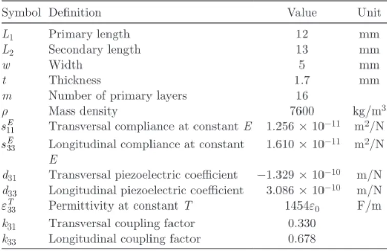
III. T E M The Rosen PT used for the modeling validation is distrib-uted by Noliac A/S (model CMT/HDE/A/25/5/1,7/2,0, Kvistgaard, Denmark) with well-known electromechanical properties and dimensions as shown in Table I.
The experimental measurements have been made to emphasize the electrical nonlinear behavior of the device. The measurements are obtained with the secondary part load-free, so it is not damped, promoting the nonlinear effect.
The admittance measurement is obtained with a two-channel signal analyzer (HP3562A, Agilent Technologies, Santa Clara, CA), which restores the fundamental part of the input current, considering the voltage supply am-plitude as constant. It should be noted that this latter assumption is not obvious because of the influence of reso-nance behavior on the supply source. Indeed, the device’s resonance induces very low input impedance, which may be less than the output impedance of the supply’s linear amplifier. Consequently, it may imply a slight variation
of the voltage amplitude. In the present characterization process, this variation has been weak and was considered insignificant as a first approximation.
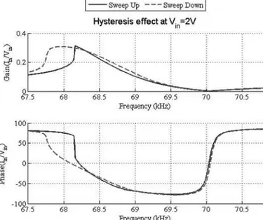
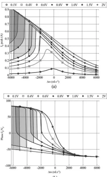
Several admittance measurements are presented in Fig. 1 according to the voltage supply amplitude. All of the characterizations concern the first longitudinal vibratory mode (i.e., λ/2 mode). Because of the presumed hysteretic behavior, the same admittance measurements were made for an up-sweeping [Fig. 1(a)] and down-sweeping [Fig. 1(b)] frequency. The hysteresis effect is more clearly illus-trated in Fig. 2 with the superimposition of the up- and down-sweeping frequency curves.
As a first assessment, it clearly appears that an in-crease in voltage supply amplitude leads to distortion of the characteristics and a downward drift of the resonance frequency. The maximal admittance amplitude is also af-fected.
TABLE I. P S R T.
Symbol Definition Value Unit
L1 Primary length 12 mm
L2 Secondary length 13 mm
w Width 5 mm
t Thickness 1.7 mm
m Number of primary layers 16
ρ Mass density 7600 kg/m3
sE11 Transversal compliance at constant E 1.256 × 10⁻¹¹ m2/N sE
33 Longitudinal compliance at constant E
1.610 × 10⁻¹¹ m2/N
d31 Transversal piezoelectric coefficient −1.329 × 10⁻¹⁰ m/N
d33 Longitudinal piezoelectric coefficient 3.086 × 10⁻¹⁰ m/N
εT33 Permittivity at constant T 1454ε0 F/m
k31 Transversal coupling factor 0.330
k33 Longitudinal coupling factor 0.678
Fig. 1. The admittance measurements according to the different voltage amplitudes with (a) up-sweeping and (b) down-sweeping frequency.
This resonance frequency drift is also noticeable on the phase graph, whereas the anti-resonant frequency remains constant as confirmed in [8]. This remark tends to confirm the preliminary assumption of not taking account of the permittivity variation of the primary side.
Finally, the verification of the thermal influence has also been carried out by using different sweep-rate fre-quencies from some millihertz per second to several hertz per second. The result of this different self-heating con-dition has given the opportunity to neglect the thermal influence compared with the main nonlinear effects. More details about the thermal effect experimentally observed are available on [13], [14].
IV. T M
The modeling developed below relies on a classical Rosen-type geometry, as shown by Fig. 3, which shows a schematic of a multilayer Rosen PT of length L0, width w,
and thickness t. The transformer consists of a transversal-ly poled driving part and a longitudinaltransversal-ly poled receiving part of lengths L1 and L2, respectively. The origin of the
coordinate system is chosen at the center of the interface between the primary and secondary portions. The driv-ing section −L1 < x1 < 0 is made of m layers with t/m
thickness. In the receiving section 0 < x1 < L2, the output
electrode at the end x1 = L2 is potentially connected to a
load resistance, RL.
A. General Model Formulation
The analytical modeling of the Rosen transformer with nonlinear behavior mainly relies on theoretical studies in [5]. In conformity with the typical one-dimensional ap-proximation of the λ/2 longitudinal vibratory mode along
a thin beam, the displacement field u = [u1 u2 u3]T and
the electric potential ϕ can be suitably approximated by
u x t u x t u x t x t u x t k k k k 1 2 3 1 1 0 0 ( , ) ( , ) ( , ) ( , ) ( , ) ( φ φ = x x1,x3, )t . (3)
Furthermore, the longitudinal component of the displace-ment field is approximated along the whole transformer length by a sine function as
u x t U k x t k L L L L 1 1 0 1 1 2 2 1 2 ( ,) sin[ ( )] ( ) , = − = + = − δ η π δ with (4)
where η is the generalized coordinate variable attached to the vibratory mechanical amplitude. The U0 constant
depends on the normalization chosen for the generalized coordinate variable η. In the present case, it is chosen to be equal to 1, as in [5]. The accurate approximation of the free vibration waveform is essential for precision of the final model. By way of comparison, (4) is graphically compared in Fig. 4 to the mechanical waveform obtained by considering the anisotropic property of the transformer
Fig. 2. Emphasis of the hysteresis effect at sufficient voltage supply am-plitude.
Fig. 3. The structure of a classical Rosen-type transformer.
along the length as described in [15]. For all the analytical expressions presented throughout this article, (4) is used.
To describe the mechanical deformations near reso-nance, the cubic theory for weak nonlinearity is consid-ered. This latter is obtained by expansion and truncation of the fully nonlinear theory into a cubic theory [17]. Con-cretely, this means that all terms up to the third power of the displacement and electric gradients or their products are included. In the present case, because the mechani-cal effects are the most significant, the terms up to cubic terms of the displacement gradient are considered and the only linear terms of the electric gradient are kept. As a consequence, the piezoelectric constitutive relations lead to the (5) and (6), distinctly expressed for the driving and receiving parts of the Rosen PT.
For the driving part,
K11=c u11 11, +e31φ,3+ξ31 1 1u2, +γ31 1 1u3, (5a)
D3 =e u31 1 1, − ε φ33 ,3. (5b)
For the receiving part,
K11=c u33 11, +h33D1+ξ11 11u2, +γ11 11u3, (6a)
φ,1=h u33 1 1, −β33D1, (6b) where K11 and Di are, respectively, the component along
the axis (Ox 1) of the first Piola stress tensor and the
elec-tric displacement. εij and γij are the constants,
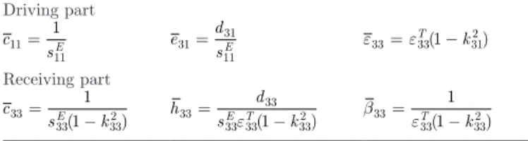
respec-tively, associated to the square and cubic terms of me-chanical displacement. The bar symbol on the coefficients of the piezoelectric material is a note to use the specific values of the transversal and longitudinal coupling modes for the primary and secondary sections, respectively. The constants are summarized in Table II.
Furthermore, the equilibrium equations relative to each part of the transformer must be added to the constitutive relations. They classically take the following form [17]: for the driving part,
K u L x
111, =ρɺɺ1 for− 1< 1<0 (7a)
D3 3, =0. (7b)
For the receiving part,
K u x L
111, =ρɺɺ1 for 0< 1 < 2 (8a)
D11, =0. (8b)
Eqs. (7b) and (8b) can be integrated to yield to an expres-sion of the electrical potential along the PT length. We
distinctly obtain expressions for the primary and second-ary sections. For −L1 < x1 < 0,
φ( , )x3t =A t xφ( ) 3+B tφ( ). (9)
For 0 < x1 < L2,
φ( , )x t1 =h u x t33 1( , )1 +Cφ( )t x1+D tφ( ), (10)
where Aϕ, Bϕ, Cϕ, and Dϕ are four integration constant
functions of time.
The Hamiltonian principle in [16], applied to the dy-namic equilibrium equations (7a) and (8a), gives
−
∫
∫
− + − = L L K u u x K u u x 1 2 0 11 1 1 1 1 0 11 1 1 1 1 0 ( , ρɺɺ)δ d ( , ρɺɺ)δ d . (11) Eq. (11) must satisfy the free-free boundary conditions and the displacement continuity at the two-part intersec-tion: K x L t K x L t u x t u x t 11 1 1 11 1 2 1 1 1 1 0 0 0 0 ( , ) ( , ) ( , ) ( , ). = − = = = = − = = + (12)The resolution of the dynamic equation by substituting (5) and (6) into (11) leads to the dynamic equation
ɺɺ η+ω η20 −e V +ξη2+γη3+ φ =0 t e C D R in , (13) with the identified parameters:
ω δ ρ 0 2 2 11 1 33 2 33 11 1 2 2 2 2 = + + − + k c L c L k c c k L L ( ) ( ) sin( ) ( ) e U L L e k D = + − 2 1 0ρ 1 2 31 δ ( ) [ sin( )] e U L L h k R = + + 2 1 0 1 2 33 33 ρ( )β [ sin( )]δ ξ ξ ξ ξ ξ δ δ ρ = + + − + + U k k k L L 0 2 31 11 31 11 1 2 4 3 3 3 3 [ ( )[ sin( ) sin( ) ]] ( ) ( ) / γ γ γ γ γ δ δ ρ / =U k k + + − k + k L 02 3 31 11 11 31 1 3 2 2 4 4 4 [ ( ) ( )[ sin( ) sin( ) ]] ( ++ L2) .
Note that in case of a laminated driving element, the equivalent input voltage must be multiplied by the num-ber of layers m, as in ɺɺ η+ω η02 +ξη2 +γη3+e Cφ =e V e = me t R D in in with in . (14)
Defining the displacement, the electric potential and voltages as a combination of cosine and sine functions, (14) can be further developed:
TABLE II. P M C. Driving part c sE 11 11 1 = e d sE 31 31 11 = ε33=ε331− 312 T k ( ) Receiving part c sE k 33 33 332 1 1 = − ( ) h d sE T k 33 33 33 331 332 = − ε ( ) β33 ε33 332 1 1 = − T k ( )
η η ω η ω ω ω ω φ φ φ φ φ = + = + = ′ ′′ ′ 1cos( ) 2sin( ) cos( ) sin( ) cos( t t C C t C t D D t)) sin( ) cos( ) cos( ) sin( + = = + ′′ ′ ′ ′′ D t V V t V V t V φ ω ω ω ω in in
out out out tt).
(15)
As an approximation, the effect of the second-order co-efficient will be neglected, as well as the effect of higher harmonics. This simplification is in conformity with the experimental measurement method explained previously (i.e., the measurement of fundamental parts of the elec-trical quantities). Consequently, considering this simpli-fication and the previously provided definition of terms leads to ( ) ( ) ( ) ω ω η γ η η η ω ω η φ φ 02 2 1 13 1 22 0 2 2 2 3 4 3 − + + + = − + + ′ ′ ′′ e C e V e C R R in in 4 4γ η( 23 +η η2 12)=0. (16)
According to the electric potential definition along the length by (9) and (10), the expression distinctly given in the driving and the receiving parts is, for −L1 < x < 0,
Vin′ cos( ),ωt (17a) and for 0 < x1 < L2, ( sin[ ] ) cos( ) ( sin[ ( )] ( ) h k x C x D t h k x C 33 1 1 1 33 2 1 η δ ω η δ φ φ φ − + + + − + ′ ′ ′′′x +D′′ t 1 φ) sin( ).ω (17b)
The boundary conditions and relations of continuity must be specified: φ φ η δ η δ φ φ ( , ) ( , ) sin( ) sin( ) 0 0 0 33 1 33 2 − + ′ ′ ′′ = ⇒ − + = − + = t t h k D V h k D in (18) φ η η φ φ φ φ ( , )L t V h C L D V h C L D V 2 33 1 2 33 2 2 = ⇒ + + = + + = ′ ′ ′ ′′ ′′ ′′ out out out.. (19)
The output voltage is deduced from the relation depend-ing on an output resistive load, RL:
V R I R Q V R C L C
V R C L C
L L
out L out L out
out out out out = = − ⇒ = − = ′ ′′ ′′ ɺ ω ω φ 2 2 φφ ′ . (20) To complete the system of equations for comparison with the experimental characterization, the expression of the input admittance is deduced from
Y I V Q V j V e u x x in in in in in in d d = = ɺ = ω
∫
( 31 11, −ε φ33 ,3) 1 2, Σ (21) which yields to Y Y t Y t Y Vp Y in in in in in in t with and ( )= cos( )+ sin( ) − = ′ ′′ ′ ′ ′ ω ω ψ η ω 2 ′′ ′ = ψ ηin 1ω− ω Vp C p , (22)where the following relation is verified:
ψin =U mwe0 31[1−sin( )]kδ =U e02 inρ(L1+L wt2) /2.
The parameter ψin corresponds to the electromechanical
conversion factor of the primary section.
The calculated capacitances of the primary and second-ary parts are
C m L w t C wt L in = 2 1 33 out = 2 33 1 ε β , . (23)
The actual equation system from (16) to (19) can be easily reduced to two equations based on variables η1 and
η2 for a numerical solving process.
This model is quite acceptable in the case of a conve-nient output load, leading to the conclusion that the main damping element is due to the output load. However, it be-comes unsatisfactory in the case of an open output circuit.
B. Considering an Open Output Circuit or High Impedance
In the case of plasma discharge applications, the output is considered to be free of electrical load before the ap-pearance of a plasma discharge. As a consequence of this condition of use, the electrical displacement expression on the receiving part (6b) can be simplified by setting the term Cϕ equal to 0. However, without an output load, it
becomes essential to include the mechanical damping to express a realistic behavior of the PT. The introduction of this damping coefficient (relative to the resonant fre-quency ω0) is obtained by introducing a mechanical
qual-ity factor, Qm. Consequently, (16) becomes
( ) ( ) ( ) ω ω η ω ωη γ η η η ω ω η ω ωη 02 2 1 0 2 13 1 22 02 2 2 0 3 4 − + + + = − + ′ Q e V Q m in in m 1 1 23 2 12 3 4 0 + + = γ η( η η ) . (24)
Thus, from (22) and (24), the admittance can be analyti-cally simulated. However, the values of Qm and γ are
re-quired to make this possible. Therefore, the identification of these two parameters is carried out using the method described in the following section.
V. T I U P
A. The Identification of the Mechanical Quality Factor
If the transformer is supplied by a low input voltage amplitude, the square and cubic terms in (24) become
negligible, leading to ignoring the influence of γ (in low signal conditions). As a consequence, the mechanical qual-ity factor can easily be measured by common methods (quadrantal frequencies, or −3-dB bypass). After admit-tance measurement and calculation, the mechanical qual-ity factor Qm can be deduced from
Q wt R U L L m m = + ω ρ 0 02 1 2 2 ( ), (25)
where Rm is the equivalent motional resistor deduced from
the common equivalent circuit RLC//C (Mason’s model).
B. The Identification of the Cubic Term Constant Factor
The identification of the parameter γ is far less trivial, and it requires some analytical simplifications. A method is introduced in [17] from the input current measurement. By manipulating (24) according to trigonometrical prop-erties and the definition of η = η12+η
2 2, (ω02 ω2)η γ η3 ω ω η ( ) . 2 0 2 2 3 4 − + + = ′ Qm e Vin in (26) Then, if the frequency ω is considered in the vicinity of resonant frequency ω0 as ω = ω0 + ∆ω and by neglecting
the term (∆ω)2, ∆ω γ η ω ω η ω − +
( )
≈ ′ 3 8 2 2 2 0 2 0 2 0 2 Q e V m in in . (27)Then, substituting (22) into (27) by neglecting the term
CinωVin′ in the vicinity of the resonance and assuming the
relation Iin = j Qω in ≈ jω ψ η0 in , the result is
V I e I Q in in in in in in ′ ≈ ± − + + 2 3 8 2 4 2 2 0 3 2 0 2 0 ψ ω γ ψ ω ω ω ω ∆ ∆ m m 2 . (28) Despite all of these approximations, it is still difficult to analytically express the dependence of the input current flow on the frequency range. As a consequence, the param-eter γ is deduced from a numerical method with a least-squares method at ∆ω = 0, giving
Vin U I L L wt I in in in in ′ ≈ ± + + 02 2 1 2 2 2 03 2 0 2 3 4 ψ ρ γ ψ ω ω ( ) Q Qm
( )
2. (29) Note that in (29), only parameters γ and ψin are sensitiveto the model’s precision. Consequently, the choice is to consider ψin as an undefined parameter in the least-squares
resolution in the same manner as γ.
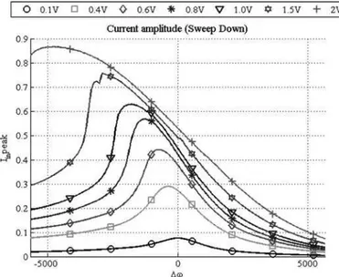
The identification of γ from (29) requires the measure-ment of the current peak values as a function of ∆ω. Thus, the peak current is obtained from the admittance mea-surements presented in Fig. 1.
Moreover, because the parameter is identified at ∆ω = 0 and this value is on the right side of the resonance peak, it appears more suitable to choose the characteris-tics using the down-sweeping frequency rather than the up-sweeping alternative. Thus, Fig. 5 is experimentally deduced.
Finally, the numerical resolution of (29) allows one to obtain the curve in Fig. 6 and
γ = −27.335×10²⁰ N/m2, ψin = −1 504. N/V,
with the squared 2-norm of the residual |res| = 0.210. Despite the analytical simplifications and simplicity of the experimental protocol, (29) appears to have a satisfac-tory accuracy.
The method presented here gives access to the γ pa-rameter, but not the γ11 and γ31 terms distinctly, as
ini-Fig. 5. The current peak as a function of ∆ω and voltage amplitude.
Fig. 6. Results of least-squares resolution for identification of the γ pa-rameter.
tially expressed in (13). Additional experimental charac-terizations should be undertaken with single ceramics to obtain these parameters and also to confirm the expres-sion of γ obtained in Section IV. Obviously, like all other parameters, the third-order constant is dependent on the sample temperature. Thus, if the experimental measure-ments are not undertaken with specific precautions, a moderate tolerance rate must be considered for the nu-meric values.
All required parameters are now available to simulate the model developed here and, thus, to discuss the results in the following section.
VI. D R
The current peak is simulated from (22) and (24), which gives the characteristics in Fig. 7(a). Fig. 7(a) is compared with the experimental curves obtained in Fig. 5.
For an easier comparison with the experimental measure-ments, the nonlinear model is illustrated in Fig. 7 by the hysteretic areas rather than by the exact multi-solution of the equation (24). The unstable frequency ranges are indicated for each characteristic by filled surfaces.
As a result, the model clearly presents an acceptable rate of accuracy regarding the current peak as a function of ∆ω. The influence of the nonlinearity can also be ob-served on the phase shift as demonstrated in Fig. 7(b) and experimentally in Fig. 1.
However, the accuracy is less obvious regarding the ad-mittance simulation according to the absolute frequency value. In fact, the most significant difference between the-oretical and experimental characteristics may be attrib-uted to the approximations considered at the beginning of the model development. Indeed, more than the one-dimen-sional approximation, the mechanical waveform chosen in free-vibration conditions implies less precision. Remember that the waveform equation (4) has been used to formu-late simpler expressions of the parameters in (13).
Consequently, an illustration of a more precise (but more computationally demanding) analytical resolution is carried out by using the expression of waveform for-mulated in [15]. The waveform equation is obtained by considering the realistic anisotropic properties resulting from the different polarization axes along the primary and secondary lengths. Thus, a brief comparison is undertaken according to the numerical values assembled in Table III.
If the capacitances are calculated by the same method, the electromechanical factor ψin and especially the
reso-nance frequency ω0 are slightly different and more in
ac-cordance with experimental results. Consequently, the model’s precision can be significantly improved by taking into account the anisotropic property along the main di-rection, as in [15], but at the cost of more complex equa-tions.
Be that as it may, the analytical method presented here and the model developed finally lead to a satisfac-tory approximation of the experimental observations on the admittance measurements, despite the simplicity of the experimental characterization method (Bode trans-fer function of the input admittance). This finally dem-onstrates the possibility of accounting for the nonlinear aspect in modeling from the beginning of transformer pre-design. However, this modeling only concerns the fun-damental part of the nonlinear behavior of the transform-er. To fully identify and validate this cubic formulation,
Fig. 7. Simulation of (a) current peak as a function of ∆ω and voltage amplitude, and (b) phase admittance.
TABLE III. T C P A T D A. Parameter Unit According to J. Yang [2] According to C. Nadal [3] ω0 rad/s 452.72 × 10³ 443.40 × 10³ ( f0) kHz 72.052 70.570 ψin N/V −0.790 −0.908 Cin nF 103.63 103.63 Cout pF 4.550 4.550
additional characterization and validation must be carried out concerning the electrical and mechanical higher har-monics.
VII. C
In this paper, an analytical method to model a piezo-electric transformer has been presented, taking into ac-count the most significant nonlinearities appearing in no-load condition, as in the configuration of a glow plasma discharge generator. The developed method is illustrated with a typical Rosen-type transformer and concerned the fundamental input current and the associated equivalent admittance. After a brief presentation of the different ori-gins of nonlinearity in piezoelectric ceramics, the operat-ing conditions of the transformer and its preliminary char-acterization have led to only considering the mechanical origin.
The modeling is based on the Hamiltonian principle by considering additional third-order terms in the piezoelec-tric constitutive equations. As a result, a system of two polynomial third-order equations was formulated. Addi-tionally, the input current and equivalent admittance were formulated analytically.
Specific experimental measurements were carried out on a test transformer with a signal analyzer to emphasize the hysteresis phenomenon of the fundamental part of the input admittance.
To simulate the analytical model, the unknown pa-rameter values—the damping factor and the third-order term coefficient—must be deduced from the measure-ments. Their identification only requires electrical input measurements in different configurations (under low- and high-signal conditions). The method is explained and the theoretical model is finally simulated and compared with the experiments.
As a result, the model developed has shown a satisfying rate of accuracy with the measurements when the com-parison is done relatively to the resonant frequency. More-over, it has been shown that the accuracy of the analytical model can be significantly improved by using a more reli-able expression of the mechanical waveform, leading to a more accurate value of the resonant frequency.
The method presented has proven the capacity to mod-el the nonlinear behavior of a piezomod-electric transformer from simple constant voltage supply measurements in up- and down-sweeping frequencies. Finally, this methodology provides the opportunity to estimate the output voltage operating range of the transformer as well as the bound-ary frequencies of the unstable range.
R
[1] K. Teranishi, S. Suzuki, and H. Itoh, “A novel generation method of dielectric barrier discharge and ozone production using a piezo-electric transformer,” Jpn. J. Appl. Phys., vol. 43, no. 9B, pp. 6733– 6739, 2004.
[2] K. Teranishi, H. Itoh, and S. Suzuki, “Dynamic behavior of light emissions generated by piezoelectric transformers,” IEEE Trans. Plasma Sci., vol. 30, no. 1, pp. 122–123, Feb. 2002.
[3] C. Nadal, F. Pigache, and Y. Lefevre, “Analytical modeling of elec-trical potential repartition on piezoelectric transformer,” in IEEE Int. Frequency Control Symp., 2010, pp. 602–607.
[4] K. Ishii, N. Akimoto, S. Tashirio, and H. Igarashi, “Influence of load resistance on higher harmonic voltages generated in a piezoelectric transformer,” Jpn. J. Appl. Phys., vol. 37, no. 9B, pp. 5330–5333, 1998.
[5] J. Yang, “Weakly nonlinear behavior of a plate thickness-mode piezoelectric transformer,” IEEE Trans. Ultrason. Ferroelectr. Freq. Control, vol. 54, no. 4, pp. 877–881, Apr. 2007.
[6] D. Damjanovic, “Ferroelectric, dielectric and piezoelectric properties of ferroelectric thin films and ceramics,” Rep. Prog. Phys., vol. 61, no. 9, pp. 1267–1324, 1998.
[7] D. A. Hall, “Review nonlinearity in piezoelectric ceramics,” J. Ma-ter. Sci., vol. 36, no. 19, pp. 4575–4601, 2001.
[8] C. Chong, W. P. Chen, H. L. W. Chan, and P. C. K. Liu, “Nonlinear behaviour of piezoceramics and piezocomposites under various ac fields,” Sens. Actuators A, vol. 116, pp. 320–328, Apr. 2004. [9] K. Ishii, N. Akimoto, S. Tashiro, and H. Igarashi, “Analysis of
non-linear phenomena in piezoelectric ceramics under high-power vibra-tion,” J. Ceram. Soc. Jpn., vol. 106, no. 6, pp. 555–558, 1998. [10] K. Ishii, S. Tashiro, and K. Nagata, “Influence of temperature on
nonlinear piezoelectricity in a piezoelectric ceramic,” Trans. Mater. Res. Soc. Jpn., vol. 28, no. 1, pp. 149–152, 2003.
[11] K. Ishii and S. Tashiro, “Effect of Sr substitution on a nonlinear piezoelectric coefficient of third-higher term in lead-zirconate-tita-nate-based piezoelectric ceramics,” Jpn. J. Appl. Phys., vol. 46, no. 10B, pp. 7048–7052, 2007.
[12] L. Landau and E. Lifchitz, The Classical Theory of Fields, 4th ed., (Course of Theoretical Physics series, vol. 1, 3rd ed.), Oxford, UK: Butterworth-Heinemann, 1976.
[13] C. H. Xu, C. H. Voo, and S. Shi, “Current oscillation of piezoelec-tric-ceramic vibrators driven by a constant high electric field,” J. Am. Ceram. Soc., vol. 88, no. 3, pp. 624–627, 2005.
[14] M. Umeda, K. Nakamura, and S. Ueha, “Effects of vibration stress and temperature on the characteristics of piezoelectric ceramics un-der high vibration amplitude levels measured by electrical transient responses,” Jpn. J. Appl. Phys., vol. 38, no. 9B, pp. 5581–5585, 1999. [15] C. Nadal and F. Pigache, “Multimodal electromechanical model of
piezoelectric transformers by Hamilton’s principle,” IEEE Trans. Ultrason. Ferroelectr. Freq. Control, vol. 56, no. 11, pp. 2530–2543, Nov. 2009.
[16] J. S. Yang, An Introduction to the Theory of Piezoelectricity. New York, NY: Springer, 2005.
[17] J. S. Yang, Analysis of Piezoelectric Devices. Singapore: World Sci-entific, 2006.
Francois Pigache was born in Auchel, France, in 1977. He received an M.S. degree in instrumenta-tion and advanced analysis in 2001, and a Ph.D. degree in electrical engineering from the Univer-sity of Sciences and Technology, Lille, France, in 2005. He joined the Laboratoire des Plasmas et de la Conversion d’Energie (LAPLACE), Toulouse, France, as an associate professor. His research there concerns multi-physic modeling, the optimi-zation of piezoelectric transformers, and alterna-tive applications of ferroelectric materials.
Clement Nadal was born in Rennes, France, in 1983. He received his Ing. degree in electrical en-gineering and his M.S. degree in 2007 from Ecole Nationale Superieure d´Electrotechnique, d´Electronique, d´Informatique, d´Hydraulique et des Telecommunications (ENSEEIHT), Toulouse, France. He received a Ph.D. degree in electrical engineering from the same institution in 2011, for his dissertation regarding analytical piezoelectric device modeling dedicated to plasma generation.