HAL Id: hal-01096593
https://hal.archives-ouvertes.fr/hal-01096593
Submitted on 19 Dec 2014
HAL is a multi-disciplinary open access
archive for the deposit and dissemination of
sci-entific research documents, whether they are
pub-lished or not. The documents may come from
teaching and research institutions in France or
abroad, or from public or private research centers.
L’archive ouverte pluridisciplinaire HAL, est
destinée au dépôt et à la diffusion de documents
scientifiques de niveau recherche, publiés ou non,
émanant des établissements d’enseignement et de
recherche français ou étrangers, des laboratoires
publics ou privés.
Temporal Alignment Model for Data Streams in
Wireless Sensor Networks Based on Causal
Dependencies
Jose Roberto Perez Cruz, Saúl Eduardo Pomares Hernández
To cite this version:
Jose Roberto Perez Cruz, Saúl Eduardo Pomares Hernández. Temporal Alignment Model for Data
Streams in Wireless Sensor Networks Based on Causal Dependencies. International Journal of
Dis-tributed Sensor Networks, Hindawi Publishing Corporation, 2014, 10 (3), pp.Article ID 938698.
�10.1155/2014/938698�. �hal-01096593�
Temporal alignment model for data streams in wireless
sensor networks based on causal dependencies
Jose Roberto Perez Cruz
1and Saul E. Pomares Hernandez
1,2,31Department of Computer Science, Instituto Nacional de Astrof´ısica, ´Optica y Electr´onica (INAOE), Luis Enrique Erro 1, C.P.
72840, Tonantzintla, Puebla, Mexico.
2CNRS, LAAS, 7 avenue du Colonel Roche, F-31400 Toulouse, France 3Univ de Toulouse, LAAS, F-31400 Toulouse, France
E-mail addresses: [email protected] (J.R. Perez Cruz), [email protected] (S.E. Pomares Hernandez).
New applications based on wireless sensor networks (WSN), such as person-locator services, harvest a large amount of data streams that are simultaneously generated by multiple distributed sources. Specifically, in a WSN this paradigm of data gener-ation/transmission is known as event-streaming. In order to be useful, all the collected data must be aligned so that it can be fused at a later phase. To perform such alignment, the sensors need to agree on common temporal references. Unfortunately, this agreement is difficult to achieve mainly due to the lack of perfectly-synchronized physical clocks and the asynchronous nature of the execution. Some solutions tackle the issue of the temporal alignment; however, they demand extra resources to the network deployment since they try to impose global references by using a centralized scheme. In this paper, we propose a temporal align-ment model for data streams that identifies temporal relationships and which does not require: the use of synchronized clocks, global references, centralized schemes or additional synchronization signals. The identification of temporal relationships without the use of synchronized clocks is achieved by translating temporal dependencies based on a time-line to causal dependencies among streams. Finally, we show the viability and the effectiveness of the model by simulating it over a sensor network with multi-hop communication.
1
Introduction
Emerging applications based on wireless sensor networks (WSN) such as remote monitoring of biosignals, multime-dia surveillance systems and person locator services [1] ubiquitously1 harvest a large amount of continuous
time-based data, as audio or video, that is generated from several sensor nodes in a distributed and concurrent way [10, 6, 18]. Specifically, the adopted transmission paradigm in such en-vironments is called event-streaming, which represents the generation and the transmission of data as a continuous stream of events reported by multiple sources [11]. In order to be useful to the application, all the collected data require a certain degree of post-processing (e.g. data fusion2).
For example, suppose that there is a network of fixed cameras along an area, which aim to monitor a person (see Figure 1). As each camera has a limited vision field, the resultant single video must be formed from multiple possi-ble video sequences, collected by different cameras. Thus, all the collected video sequences will be processed/fused to produce useful information (see Figure 1).
To perform some kind of analysis or processing, all the data originated through the event-streaming must be
tem-1In this context, the term ubiquitous refers to the capacity to collect
information from several places at the same time.
2Data fusion refers to the alignment, association, correlation, filtration
and aggregation of the collected data [9, 3].
Figure 1: Scenario of a person monitoring system.
porally aligned in some way to make them functional and coherent. To achieve this, the sensors in the network may need to agree on some common temporal references to the whole system [8, 4, 10, 14]. Unfortunately, the characteris-tics and restrictions of a WSN make it difficult to establish such references. This is mainly due to: 1) the resources’ constraints, 2) the channel variability, 3) the dynamicity in the topology, 4) the lack of perfectly synchronized physical clocks, 5) the absence of shared memory, and 6) the asyn-chronous nature of the event-streaming [6].
In order to avoid the use of synchronized clocks, a clock-free alignment approach for data streams was proposed in [14]. This solution is based on the fact that in most sensor networks, some sensor nodes act as intermediate nodes to aggregate or to collect the data streams which are later sent to another sensor or sink. Assuming the previous
commu-nication scheme, the approach has shown that aligning the data streams on the intermediate nodes without synchroniz-ing the clocks of all sensors is sufficient. Nevertheless, this solution requires a synchronization server that broadcasts synchronization signals to the sensors to establish a global reference, and it also needs dedicated devices (data servers) to align the streams according to the broadcasted signals. These two additional requirements imply extra network re-sources.
In this paper, we propose a new model called Event-Streaming Logical Mapping (ES-LM), for the temporal data alignment in WSNs. The ES-LM model is based on the event-streaming paradigm, the logical mapping model [20] and the data alignment approach described in [17]. The ES-LM uses pairwise interactions between nodes based on the happened-before relation [12]. The ES-LM performs the data alignment by translating temporal dependencies among streams, based on a time-line, to causal dependen-cies. Such translation allows us to construct a virtual time-line. By using the resulting virtual time-line we can avoid: 1) the use of synchronized clocks, 2) the use of global ref-erences, 3) the use of centralized schemes, and 4) the use of additional synchronization signals. Finally, we show the viability and the effectiveness of the model by simulating it over a sensor network with multi-hop communication.
This paper is structured as follows. Section 2 presents the system model and the background, including our definition of the event-streaming as an abstract data type. Section 3 presents a description of the proposed temporal data align-ment model for event-streaming. In Section 4 we present the analysis of the model and the simulation results. Fi-nally, Section 5 presents the conclusions.
2
Preliminaries
2.1 System model
We specify a WSN as a distributed system, which consists of three main components:
• Processes. Each entity associated to the WSN (sen-sors or sink) is represented as an individual process. Hence, a WSN is a set of processes P = {pi,pj, ...}that
communicate with each other by message passing. A process can only send one message at a time.
• Messages. We consider a finite set of messages M sent by a process p ∈ P. Such messages contains the samples of audio, video or many other physical signals that each sensor collects. Henceforth, we will refer to a sample as a message. For a message, the sample time
xis the time instant at which a process p conducts such a sample. Thus, each message m ∈ M can be identified as m(p, x).
• Events. An event represents an instant execution per-formed by a process. For our problem of data align-ment, we only consider the send and delivery events.
1. The send event refers to the emission of a mes-sage executed by a process.
2. The delivery event refers to the execution per-formed by a process to present the received in-formation to an application or another process. Let m be a message. We denote by send(m) the emis-sion event and by delivery(p, m) the delivery of m to the process p. The whole set of events in the sys-tem is the finite set: E = {send(m) : m ∈ M} ∪ {delivery(p, m) : m ∈ M, p ∈ P}.
Furthermore, for the transmissions in a WSN we consider two main characteristics:
• Transmission delay. For a message m ∈ M there is a time period to contend for the transmission media and the network propagation.
• Synchronization error of two samples. This refers to the difference between the local time reference as-signed at the reception, which can be used to estimate the sample time, and the sample time of the source. 2.2 Background and Definitions
A suitable way to order events in an asynchronous dis-tributed system is the happened-before relation (HBR) de-fined by Leslie Lamport [12]. This relation establishes the rules to determine whether an event is the cause or the effect of another event, without using global references.
The HBR is a strict partial order on events, defined as follows:
Definition 1 The happened-before relation, “→”, is the
smallest relation on a set of events E satisfying the follow-ing conditions:
1. If a and b are events belonging to the same process, and a was originated before b, then a → b.
2. If a is the sending of a message by one process, and b is the reception of the same message in another process, then a → b.
3. If a → b and b → c, then a → c.
Based on Definition 1, Lamport defines that a pair of events is concurrently related “a ∥ b” as follows:
Definition 2 Two events, a and b, are said to be concurrent
if a ↛ b and b ↛ a; it is denoted by a ∥ b [12].
Immediate dependency relation (IDR). The IDR is the
transitive reductionof the HBR [19]. The IDR is defined as follows:
Definition 3 Two events a, b ∈ E have an immediate
de-pendency relation (denoted by “↓”) if:
Note that an event a causally and immediately precedes an event b, if and only if, there is no other event c ∈ E, such that c belongs to the causal future of a and to the causal past of b.
Intervals. An interval is a set of events which occur dur-ing a period of time. If the events that compose an interval satisfy a certain order, then such interval is called ordered interval. The works of Shimamura et al. [21] and Pomares et al. [20] define the following ordered interval composi-tion.
Definition 4 Let X be an interval of sequentially-ordered
events at a process pi; X ⊂ E, and x−,e, x+ ∈ X; where x−
is the left endpoint and x+is the right endpoint of interval
X, such that ∀e ∈ X, x−→ e → x+and x−,e, x+,e.
When |X| = 1, this implies that x−= x+; in this case, x−
and x+are denoted indistinctly by x.
Happened-before relation for intervals. Lamport estab-lishes in [13] that an interval A happens before another interval B if all the elements that compose an interval A causally precede all the elements of interval B.
Definition 5 The causal relation “→” is established at a
set level by satisfying the following conditions: 1. A → B if a → b, ∀(a, b) ∈ A × B,
2. A → B if ∃ C |(A → C ∧ C → B).
According to Definition 4 and Pomares et al. [20], the happened-before relation in regard to ordered intervals can be expressed only in terms of the endpoints as follows: Property 1 Let A, B and C be sets of sequentially-ordered
events. The set of events A occurs before the set of events B if any of the following conditions are satisfied:
1. A → B if a+→ b−
2. A → B if ∃C, such that a+→ c−∧ c+→ b−
Definition 6 Let A and B be two ordered intervals. A and
B are said to be simultaneous (denoted by A|||B) if the fol-lowing condition is satisfied [20]:
A|||B i f a−∥ b−∧ a+∥ b+
The definition above means that one interval A can take place at the “same time” as another interval B.
2.2.1 The logical mapping model
The logical mapping model introduced in [20] is useful to represent pairwise interactions between processes. Such model expresses temporal relations between sets of events in terms of the happened-before relation for intervals.
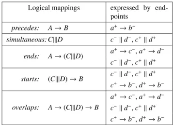
Table 1: Logical mappings expressed by endpoints Logical mappings expressed by
end-points precedes: A → B a+→ b− simultaneous: C|||D c−∥ d−, c+∥ d+ ends: A →(C|||D) a +→ c−, a+→ d− c−∥ d−, c+∥ d+ starts: (C|||D) → B c −∥ d−, c+∥ d+ c+→ b−, d+→ b− overlaps: A →(C|||D) → B a+→ c−, a+→ d− c−∥ d−, c+∥ d+ c+→ b−, d+→ b−
The logical mapping translation involves every pair X,
Y of intervals of a temporal relation. Each pair is seg-mented into four subintervals : A(X, Y), C(X, Y), D(X, Y), and B(X, Y), as shown in Table 1.
The logical mapping model identifies five logical map-pings, which are sufficient to represent all possible tem-poral relations between continuous media (interval-interval relations [2]), discrete media (point-to-point relations), and discrete-continuous media relations [15].
2.2.2 Event-streaming abstract data type
We propose a definition of the event-streaming oriented to the data alignment problem. Assuming that an event-streaming is composed of several events, we begin by defin-ing the concept of an atomic event.
Atomic event. An atomic event indicates that an entity has sent or delivered a message containing a sample. In other words, an atomic event indicates that a portion of data has been collected from the environment.
Definition 7 An atomic event is a tuple e(pj,m(pi,x)),
where pj refers to the process where the event is executed
and m(pi,x) is a message (m ∈ M) originated by process
pi.
As we stated above, we consider only two types of events: send and delivery. We denote the atomic delivery event by
delivery(pj,m(pi,x)), and we denote the atomic send event
only by send(m(pi,x)) since pi= pj.
Based on the concept of atomic event, for our solu-tion we distinguish two kinds of data streams generated by the nodes in a WSN: the local-streams and the
event-streamings.
Local-streams. In a WSN, each process generates a cer-tain number of atomic events throughout the communica-tion process. When some of these events are generated
se-quentially by a process piduring a period of time, we say
that the process pi ∈ P has generated a local-stream. We
formally define a local-stream as follows:
Definition 8 A local-stream is a poset (Si, →i) where Siis
a finite set of atomic events Si = {e1,e2, ...en} generated
by the process pi ∈ P and arranged according to the local
causal relation →i.
A local-stream can be expressed by its endpoints, simi-larly to the intervals (see Definition 4). For a local-stream
Si ={e1,e2, ...en}, the endpoints are S−i = e1and S+i = en.
The endpoint S−
i refers to the beginning of the local-stream,
while S+
i refers to its end.
Event-streamings. An event-streaming is a collection of subsets of local-streams generated by different processes. Such subsets of local-streams are grouped and arranged ac-cording to their causal dependencies into sets denoted as
QRq
q , where Rqdenotes the set of identifiers of the processes
that generated the events in QRq
q . Thus, in a generic way, an
event-streaming ESΘcan be viewed as the general causal
structure:
ESΘ= QR11→ QR22→ · · · → QRm−m−11→ QRmm
We formally define an event-streaming as follows: Definition 9 An event-streaming is a poset (ESΘ, →)
where ESΘ is a finite set of subsets of events ESΘ =
{QR1
1 ,Q
R2
2 , ...,Q
Rm
m} arranged according to the causal
rela-tion →; Θ is the set of the identifiers of the processes that generated the events; and each QRq
q ∈ ESΘis a subset of
events generated by the processes whose identifiers form the set Rq.
Within an event-streaming each set QRq
q is a collection
of subsets of local-streams Ωi, Ωj, ..., Ωk, where Ωi ⊆ Si,
Ωj⊆ Sjand Ωk⊆ Sksuch that Ωi|||Ωj||| · · · |||Ωk(i, j, ..., k ∈
Rq). Furthermore, the events in any set Ως are arranged
according to the local causal relation →ς, which form the
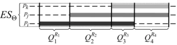
poset (Ως, →ς). For example, suppose that three processes
pi, pj and pk generated three local-steams as depicted in
Figure 2. When a process collects such local-streams, it constructs four subsets: Q{i}1 containing events exclusively generated by pi, Q
{i, j}
2 containing events generated by piand
pj, Q
{i, j,k}
3 containing events generated by pi, pjand pkand
Q{ j,k}4 containing events generated by pjand pk.
pi pj pk Q 1 R1 Q 2 R2 Q 3 R3 Q 4 R4
Figure 2: Representation of the subsets of an event-streaming.
We note that in a similar way to the local-streams and the intervals, each subset QRq
q can be expressed by its endpoints.
However, unlike local-streams and intervals, the endpoints of a subset QRq
q are sets of events formed by the endpoints
of each set Ως ∈ Q
Rq
q , respectively. Thus, when a set Q Rq
q
contains events generated by the processes pi, pj and pk,
we denote the left set endpoint as−QRq
q which is composed as follows: −QRq q ={ω−i, ω − j, ω − k}, where ω − i ∈ Ωi, ω − j ∈ Ωj and ω−
k ∈ Ωk. Likewise, we denote the right set endpoint as
+QRq
q which is composed as follows:+Q Rq q ={ω+i, ω + j, ω + k}, where ω+i ∈ Ωi, ω+j ∈ Ωjand ω+k ∈ Ωk.
3
Temporal
data
alignment
for
event-streaming
3.1 The problem of data alignment for event-streaming
Based on the definition of the data stream alignment prob-lem given in [14], we define the probprob-lem of data alignment for event-streaming as follows.
Definition 10 Data alignment problem for event-streaming: Given a set of local-streams: {S1,S2,S3, ...},
and considering a certain maximum transmission delay, the problem is to assign a temporal reference that can be used as an estimated sample time for each interested message, such that for every two messages m(pi,x) and
m(pj, y), their synchronization error is bounded.
For our solution, the messages of interest are the causal messages sent within an event-streaming. Explicitly, they are the endpoints of the subsets QRq
q . In this sense, the
synchronization errorestablishes the temporal distance be-tween the execution of a pair of messages of interest. 3.2 Event-streaming logical mapping model (ES-LM) The native logical mapping identifies five logical mappings:
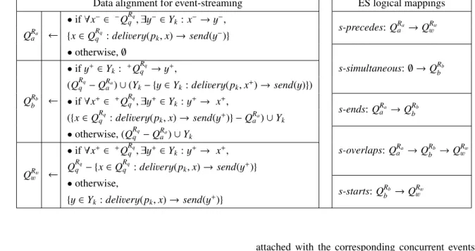
precedes, simultaneous, ends, starts and overlaps to deter-mine how two intervals (local-streams) are related. How-ever, for our problem this covers only the base case, which is the alignment of streams whose events have all been gen-erated by a single process. In the following sections, we present an extension to the native logical mapping called event-streaming logical mapping model (LM). The ES-LM establishes how an event-streaming ESΘ (a stream
composed by events generated by several processes) is re-lated to a local-stream Ykin order to determine the events
that have causal dependencies and the subsets of events that concur. To achieve this, it is necessary to determine how each subset QRq
q ∈ ESΘ is related to a local-stream Yk.
We note that any subset QRq
q is considered as a
sub-event-streaming. In our ES-LM model, without loss of generality, it is assumed that −QRq
q → Yk− or
−QRq
q || Yk−. Therefore,
when a subset QRq
q is aligned to a local-stream Yk, a new
sub-event-streaming is generated according to the left col-umn of Table 2. The resultant sub-event-streaming has the following general causal structure:
QRa a → Q Rb b → Q Rw w
From this causal structure, five new logical mappings are identified. These logical mappings represent all the ways that an event-streaming can be related to a local-stream. These new logical mappings are: precedes,
s-simultaneous, s-ends, s-overlaps and s-starts (see right col-umn of Table 2).
The ES-LM is the core of the data alignment scheme that we propose, which is presented in the following section. 3.3 Data alignment description
The data alignment process is described through four stages as follows.
A.1 Initial stage: alignment of two local-streams Ini-tially, we have two local-streams Xcand Yd (Xc− → Yd−or
X−
c || Yd−). Applying the native logical mapping, we generate
the first event-streaming ESΘas follows.
We construct a first subset Q{c}1 with the first non-concurrent events in Xc(see Table 3). To determine those
non-concurrent events, we need to identify all the events
x ∈ Xcthat precede the beginning of Yd(see Figure 3).
Then, according to Table 3, we proceed to construct a second subset Q{c,d}2 with the concurrent events between Xc
and Yd. The concurrent segments of both local-streams will
be bounded by the beginning of Yd and the end of any of
the two local-streams (see Figure 4).
t
Yd
X c
Q 1{c}
Figure 3: Aligning the first subset of the first event-streaming.
t
Yd
X c
Q 2{c,d}
Figure 4: Aligning the second subset of the first event-streaming.
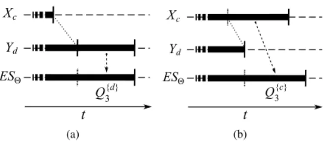
The last subset Q{w}3 is constructed depending upon which local-stream finishes first. If Xcfinishes first, the last subset
will contain the remaining events of Yd(see Table 3).
Oth-erwise, the last subset will contain the remaining events of
Xd (see Table 3). These two cases are illustrated in Figure
5. t Yd X c Q 3{d} (a) t Yd X c Q 3{c} (b)
Figure 5: Aligning the last subset of the first event-streaming. (a) Xcfinishes first (b) Ydfinishes first.
Therefore, the first event-streaming has the general causal structure ESΘ = Q{c}1 → Q{c,d}2 → Q{w}3 , where w
may be c or d.
Table 3: A.1 Alignment of two local-streams
Q{c}1 ← • if x−∈ X c, y−∈ Yd: x−→ y−, {x ∈ Xc: delivery(pd,x) → send(y−)} • otherwise, ∅ Q{c,d}2 ← • if x+∈ X c, y+∈ Yd: x+→ y+,
(Xc−Q{c}1 )∪(Yd−{y ∈ Yd: delivery(pd,x+) → send(y)}) • if x+∈ X c, y+∈ Yd: y+→ x+, ({x ∈ Xc: send(x) → delivery(pc, y+)} − Q{c}1 ) ∪ Yd • otherwise, (Xc− Q{c}1 ) ∪ Yd Q{w}3 ← • if x+∈ X c, y+∈ Yd: y+→ x+, Xc− ({x ∈ Xc: send(x) → delivery(pc, y+)} − Q{c}1 ) • otherwise, {y ∈ Yd: delivery(pd,x+) → send(y)})
Once the first stage has finished, we proceed to align two streams: an streaming and a local-stream. The event-streaming is labeled as the set Xβ, where β is the set of
iden-tifiers of the processes that generated the events, while the local-stream is labeled as Yk, where k is the identifier of
the local process. Each resultant event-streaming is merged with the next most-left local stream Yk according to the
causal dependencies among the events of Ykand the
event-streaming Xβ.
Using Xβ and Yk, we construct a new event-streaming
forming the subsets QTq
q of the general causal structure
ESΘ = QT11 → QT22 → · · · → QTn−n−11 → QTnn by detecting
the concurrences between Xβand Yk.
Assuming that the initial stage was accomplished, the logical mapping proceeds according to the three stages that are detailed below.
B.1 Aligning the first subsets of events without concur-rences between an event-streaming and a local-stream In the first step, we determine if there are some subsets
QRa
a ∈ Xβ that precede the local-stream Ykto form the first
subsets of the new event-streaming (see stage B.1 of Table 4). These subsets have events that are not concurrent with the events of Ykand are integrated directly to the new
event-streaming to form the first subsets QTa
Table 2: Event-streaming logical mapping
Data alignment for event-streaming ES logical mappings
QRa a ← • if ∀x−∈ −QRq q , ∃y−∈ Yk: x−→ y−, s-precedes: QRa a → Q Rw w {x ∈ QRq q : delivery(pk,x) → send(y−)} • otherwise, ∅ s-simultaneous: ∅ → QRb b QRb b ← • if y+∈ Y k: +Q Rq q → y+, (QRq q − Q Ra a ) ∪ (Yk− {y ∈ Yk: delivery(pk,x+) → send(y)}) • if ∀x+∈ +QRq q , ∃y+∈ Yk: y+→ x+, s-ends: QRa a → QRbb ({x ∈ QRq q : delivery(pk,x) → send(y+)} − QRaa) ∪ Yk • otherwise, (QRq q − Q Ra a ) ∪ Yk s-overlaps: QRa a → Q Rb b → Q Rw w QRw w ← • if ∀x+∈ +QRq q , ∃y+∈ Yk: y+→ x+, QRq q − {x ∈ Q Rq q : delivery(pk,x) → send(y+)} • otherwise, s-starts: QRb b → Q Rw w {y ∈ Yk: delivery(pk,x) → send(y+)} 6).
t
Yk X ✁ Q 1 R1 Q 2 R2 Q 3 R3 Q 1 T1 Q 2 T2 Q 3 T3 Q 4 T4Figure 6: Aligning the first subsets of events of an event-streaming
If a subset QRa
a ∈ Xβhas events that are concurrent with a
part of the local-stream Yk, this subset is segmented to form
two new subsets for the new event-streaming ESΘ. The
new subset QTa
a , the first of the two new subsets, will
con-tain the part of QRa
a whose events have no concurrence. To
determine the events without concurrences, it is necessary to identify the event x ∈ QRa
a that immediately precedes the
beginning of the local-stream Yk, (see line 1.2 of Table 4).
For the example depicted in Figure 6, the new subset QTa
a
corresponds to the subset QT3
3 . The remaining events of
QRa
a are aligned as stated in the following stage.
B.2 Aligning the subsets of events with concurrences be-tween an event-streaming and a local-stream If during stage B.1 a subset QRa
a was detected containing events
con-current with a portion of the local-stream Yk, such a portion
of Ykis attached to the part of QRaa with concurrent events
to form a new subset QTc
c (see line 2.1 of Table 4).
Once the beginning of the concurrent parts of both streams are detected, according to stage B.2 of Table 4 (lines 2.2 and 2.3), all the subsequent subsets QRb
b ∈ Xβare
attached with the corresponding concurrent events of Yk,
until one of the two streams finishes. This means that for each subset QRb
b in the concurrent part of Xβ, a new subset
QTc
c will be constructed for the new event-streaming ESΘ
(see Figure 7).
t
Yk X ✁ Q 3 R3 Q 4 R4 Q 5 R5 Q 6 R6 Q 3 T3 Q 4 T4 Q 5 T5 Q 6 T6 Q 7 T7Figure 7: Aligning the subsets of events with concurrences.
The final subsets of the resulting event-streaming will be constructed depending upon which stream finishes first.
If the local-stream Yk finishes first (y+ → Xβ+), the last
concurrent subset QRb
b ∈ Xβ can contain some events that
are concurrent with Yk and other events that have no
con-currence (see Figure 8). If this is the case, QRb
b needs to be
segmented to construct two new subsets for the new event-streaming ESΘ. The new subset QTcc, the first of the two
new subsets, will contain the concurrent part of QRb
b and
the concurrent events of Yk. To determine such concurrent
events, it is necessary to identify the event x ∈ QRb
b that
im-mediately precedes the end of the local-stream Yk and the
concurrent part of the local-stream (see line 2.4 in Table 4). For the example depicted in Figure 8, the new subset QTc
c
corresponds to subset QT7
7 . The remaining events of Q
Rb
b are
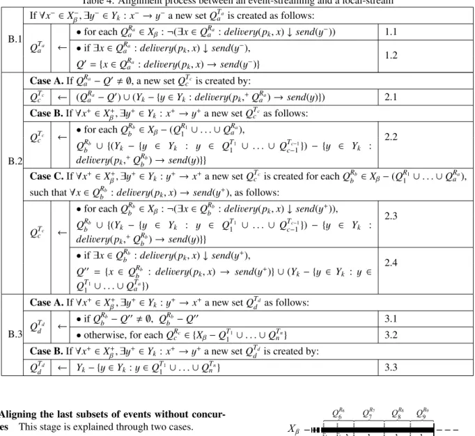
Table 4: Alignment process between an event-streaming and a local-stream
B.1
If ∀x−∈ X−β, ∃y−∈ Yk: x−→ y−a new set QTaais created as follows:
QTa a ← • for each QRa a ∈ Xβ: ¬(∃x ∈ Q Ra a : delivery(pk,x) ↓ send(y−)) 1.1 • if ∃x ∈ QRa a : delivery(pk,x) ↓ send(y−), 1.2 Q′={x ∈ QRa a : delivery(pk,x) → send(y−)} B.2 Case A. If QRa
a − Q′,∅, a new set QTccis created by:
QTc c ← (Q Ra a − Q′) ∪ (Yk− {y ∈ Yk: delivery(pk,+QRaa) → send(y)}) 2.1 Case B. If ∀x+∈ X+ β, ∃y +∈ Y
k: x+→ y+a new set QTcc as follows:
QTc c ← • for each QRb b ∈ Xβ− (Q R1 1 ∪ . . . ∪ Q Ra a ), 2.2 QRb b ∪ {(Yk − {y ∈ Yk : y ∈ Q T1 1 ∪ . . . ∪ Q Tc−1 c−1}) − {y ∈ Yk : delivery(pk,+QRbb) → send(y)}} Case C. If ∀x+∈ X+ β, ∃y +∈ Y
k: y+→ x+a new set QTcc is created for each QbRb∈ Xβ− (QR11∪ . . . ∪ QRaa),
such that ∀x ∈ QRb b : delivery(pk,x) → send(y + ), as follows: QTc c ← • for each QRb b ∈ Xβ: ¬(∃x ∈ Q Rb b : delivery(pk,x) ↓ send(y +)), 2.3 QRb b ∪ {(Yk − {y ∈ Yk : y ∈ Q T1 1 ∪ . . . ∪ Q Tc−1 c−1}) − {y ∈ Yk : delivery(pk,+QRbb) → send(y)}} • if ∃x ∈ QRb b : delivery(pk,x) ↓ send(y +), 2.4 Q′′ = {x ∈ QRb b : delivery(pk,x) → send(y +)} ∪ (Y k− {y ∈ Yk : y ∈ QT1 1 ∪ . . . ∪ Q Ta a }) B.3
Case A. If ∀x+∈ X+β, ∃y+∈ Yk: y+→ x+a new set QTddas follows:
QTd d ← • if QRb b − Q ′′,∅, QRb b − Q ′′ 3.1
• otherwise, for each QRc
c ∈ {Xβ− QT11∪ . . . ∪ QTnn} 3.2
Case B. If ∀x+∈ X+β, ∃y+∈ Yk: x+→ y+a new set QTddis created by:
QTd d ← Yk− {y ∈ Yk: y ∈ Q T1 1 ∪ . . . ∪ Q Tn n } 3.3
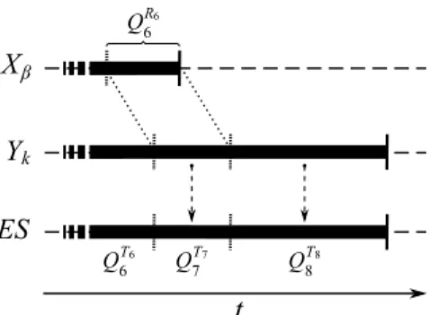
B.3 Aligning the last subsets of events without concur-rences This stage is explained through two cases.
Case A. Yk finishes before Xβ. If at the end of stage
B.2, the last subset QRb
b was segmented, the second created
subset, denoted as QTd
d , will contain the remaining
non-concurrent events of QRb
b (see line 3.1 of Table 4). In the
example of Figure 8, such subset QTd
d corresponds to the
subset QT8
8 .
The fact that the local-stream Ykfinishes first (y+→ Xβ+)
implies that the concurrent parts of both streams finish along with Yk. Therefore, according to line 3.2 of Table
4, the remaining subsets QRc
c ∈ Xβwill become the last
sub-sets QTd
d ∈ ESΘ. In the example of Figure 8, the last subsets
QTd
d are the subsets Q T9 9 , Q T10 10 and Q T11 11.
Case B. Xβ finishes before Yk. The fact that the
event-streaming Xβ finishes first (Xβ+→ y+, y+ ∈ Yk) means that
the concurrent parts of both streams finish along with the event-streaming Xβ. After the last subset QTcc ∈ ESΘwas
constructed with the concurrent events of Xβ and Yk, only
one more subset QTd
d is constructed according to line 3.3 of
Table 4. Such subset QTd
d will contain the remaining events
of the local-stream Yk. In the example of Figure 9, the last
subset QTd
d corresponds to the subset Q T8 8 .
t
Yk X ✁ Q 6R6 Q 7R7 Q 8R8 Q 9R9 Q 7 T7 Q 8 T8 Q 9 T9 Q 10 T10 Q 11 T11Figure 8: Aligning the last subsets of events without con-currences when y+→ X+
β.
The event-streaming logical mapping will continue until there are no more concurrent local-streams to be merged.
In terms of data alignment, we note that by the way in which the subsets of events are constructed and causally ordered, each resultant event-streaming ESΘis a finite
col-lection of disjoint subsets QTq
q arranged one after another
without interruption. This arrangement of subsets QTq
q in an
ESΘallows us to establish a relative time-line, where each
subset QTq
t
ES
Y
kX
✁ Q 6R6 Q 7 T7 Q 8 T8 Q 6 T6Figure 9: Aligning the last subsets of events without con-currences when X+
β → y +.
subsets QTq
q are disjoint implies that each event in an
event-streaming belongs to a unique subset QTq
q , and therefore it
is located at a specific time-slot.
4
Analysis and results
4.1 Proof of the temporal data alignment
In this section we prove that by following the ES-LM model, the sequential arrangement of subsets of events that compose an event-streaming establishes a virtual time-line, where each subset represents a unique time-slot and each event is aligned with respect to only one of them.
Theorem 1 The arrangement of subsets QRq
q in an
event-streaming establishes a virtual time-line, where each subset QRq
q represents a unique time-slot and each event belongs to
a unique time-slot.
Proof. We divide this proof into two parts. In the first part we prove that an event-streaming is a causal arrangement of subsets of events that establishes a time-line. In the second part we prove that each subset QRq
q in an event-streaming
represents a unique time-slot.
Part I. To demonstrate that an event-streaming is a causal arrangement of subsets of events that establishes a time-line, we formulate and prove the following Lemma: Lemma 1 An event-streaming is a causal arrangement of
subsets of events that establishes a time-line.
Before proving Lemma 1, we need to consider the fol-lowing. Definition 8 states that a local-stream is a poset (Si, →), where Siis a set of atomic events generated by the
same process. Thus, (Si, →) is a sequence Si = {eα →
eα+1 → · · · → en−1 → en}. The fact that the events of Si
are arranged by → implies that each event happens before another at a different instant, which determines a chrono-logically order. Therefore, a local-stream Si represents a
time-line for a process i.
Proof of Lemma 1 We demonstrate Lemma 1 by a di-rect proof. According to the ES-LM (Tables 2, 3 and 4)
during the data alignment, the subsets of events that com-pose a new event-streaming ESβ, are formed by
segment-ing two streams (a local-stream and an event-streamsegment-ing or two local-streams). From Tables 3 and 4 (specifically, stage B.1; cases B and C of stage B.2; and stage B.3) we have that a segmentation is triggered by the identification of an endpoint which determines the beginning or the end-ing of an overlap between a pair of streams. Whichever the case, each segmentation establishes the creation of two new subsets QRu−1
u−1 and Q
Ru
u . Let Ycbe a local-stream and
let X denote a local-stream or an event-streaming such that ∀x−∈ X, ∃y−∈ Y
c : x− → y−. Assuming that e∗(e∗ ∈ Yc
or e∗ ∈ X) is the endpoint (e∗ = y−∨ e∗ = y+∨ e∗ = x+),
whose identification triggered the segmentation, ∀x+ ∈ X,
QRu−1
u−1 and Q
Ru
u are constructed according to one of the three
following cases: 1. if e∗ ∈ Y
c, e∗ = y−, and x− → y−then QRu−u−11 ={x ∈
X : delivery(pc,x) → send(e∗)} and QRuu ={e∗} ∪ {x ∈
X : send(e∗) → delivery(pc,x)} ∪ {y ∈ Yc: send(y) →
delivery(pc,x+)};
2. if e∗ ∈ X, e∗ = x+, and x+ → y+then QRu−1
u−1 ={e ∗} ∪
{x ∈ X : delivery(pc,x) → delivery(pc,e∗)} ∪ {y ∈
Yc: send(y) → delivery(pc,e∗)} and QRuu ={y ∈ Yc :
delivery(pc,e∗) → send(y)};
3. if e∗ ∈ Y
c, e∗ = y+, and y+→ x+then QRu−u−11 ={e∗} ∪
{x ∈ X : delivery(pc,x) → send(e∗)} ∪ {y ∈ Yc :
send(y) → send(e∗)} and QRu
u ={x ∈ X : send(e∗) →
delivery(pc,x)}.
In each of these three cases, happened-before relation-ships are established among the left endpoints of QRu−1
u−1 and
the right endpoints of QRu
u . This means that for a pair of
subsets QRu−1 u−1 and Q Ru u (Q Ru−1 u−1 ,Q Ru u ∈ ESβ) we have that ∀(ω+ i, ω − k) ∈ +QRu−1 u−1 × −QRu u : ω+i → ω − k (i, k ∈ β).
Further-more, all the events that compose QRu−1
u−1 and Q
Ru
u are
ex-tracted from local-streams by preserving their causal order. Thus, let ωiand ω+i be two events such that ωi, ω+i ∈ Ωi,
Ωi∈ QRu−u−11 and Ωi⊆ Si(for any local-stream Si) if ωi,ω+i
then ωi → ω+i. By the transitive property of the HBR
we have that ωi → ω−k, ∀ω−k ∈ QRuu. Moreover, for any
event ωk ∈ Q Ru
u , ωk ,ω−k, ω
−
k → ωk; thereby, transitively
ωi→ ωk. Therefore, by Definition 5 we have QRu−u−11→ QRuu.
Thus the subsets of an event-streaming are chronologically ordered representing a time-line, where each subset QRq
q is
a time-slot. □
Corollary 1 Each subset QRq
q ∈ ESΘ represents a
time-slot.
Part II. To demonstrate that each subset QRq
q in an
event-streaming represents a unique time-slot, we formulate and prove the following Lemma:
Lemma 2 Each subset QRq
q represents a unique time-slot,
therefore, any pair of subsets QRu
an event-streaming ESΘ, is disjoint.
∀ QRu
u ,QRvv∈ ESΘ,u , v: QRuu∩ QRvv =∅
Proof of Lemma 2We prove Lemma 2 by contradiction. Therefore, we suppose that ∀ QRu
u ,Q Rv v ∈ ESΘ,u , v: QRuu∩ QRv v ,∅, i.e., ∃xµ: xµ∈ Q Ru u ∧ xµ∈ Q Rv v .
According to the ES-LM model, the subsets QRq
q of
an event-streaming are created by aligning two local streams or aligning a local stream with an event-streaming. Whichever way an event-streaming is generated, a subset
QRu
u must be related to another QRvv (u , v) according to
one of the five logical mappings described in Table 2. This means that for any eµ∈ Q
Ru
u and any cµ ∈ Q
Rv
v , eµ → cµor
cµ→ eµ. Thus, if there is xµsuch that xµ∈ Q
Ru
u ∧ xµ∈ Q
Rv
v ,
implies that xµ → xµ is a contradiction, according to the
assumptions by which the happened-before relation are de-fined (systems in which an event can happen before itself do not seem to be physically meaningful). □
4.2 Simulation results
We have simulated the temporal data alignment model for event-streaming using the Castalia simulator [5]. The simu-lation scenario is within a set of 50 nodes that were arranged into multi-hop paths, where the nodes are separated by dis-tances between 5 and 10 meters in a field of 200 × 200 me-ters. Through each multi-hop path, a node reaches the sink helped by up to 10 relay nodes. With this arrangement, each relay node aligns the streams generated by the predecessor nodes in the path in such a way that if there exist nr nodes
behind a node pi, pialigns at most nrstreams.
For the simulation, we implemented the model using the well-known vector clock structure [16, 7] to identify and preserve the causal relations among events. Therefore, we obtain a computational cost as well as communication and storage overheads of O(nr), where nris the number of nodes
that are related to a certain node during the data transmis-sion.
To transmit a local-stream we use two types of causal messages: begin and end, and a type of FIFO message:
f i f o pwhich does not carry any causal information. So, a process pigenerates a local-stream Siby sending a begin
message (S−
i) followed by certain number of f i f o p
mes-sages. Finally, to notify a process pjthat the transmission of
the local-streaming has been finished, the process pisends
an end message (S+i).
The simulation was configured with the TMAC protocol for the MAC sublayer and the CC2420 radio protocol for wireless transmissions. The data payload for the Applica-tion layer packets was fixed to 2000 bytes.
In the simulation scenario, each node generated a random number of local-streams throughout the simulation. Each generated local-stream was composed by a random number of messages between 9 and 100, that were generated using sampling rates between 25 and 1000 milliseconds.
In order to measure and to show that the synchronization error is bounded, we took the simulation time as a global
clock. We note that the simulation time was not used in the ES-LM. The ES-LM use only the causal dependencies between the event-streamings to perform the data alignment and do not use any kind of physical time.
At each hop we took the causal messages begin and end exchanged during the transmissions of the local-streams to determine the synchronization error between a pair of streams.
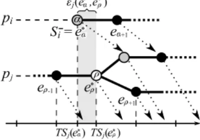
Let e∗α denote the send event executed by process pi to
transmit the causal message m(pi, α) (begin or end), and
let e∗
ρ be the send event executed by process pj to
trans-mit m(pj, ρ), which is the latest aligned message before the
reception of m(pi, α); when pjreceives m(pi, α), the
syn-chronization error of a pair of local-streams is determined by the difference between the sampling time of m(pi, α) and
m(pj, ρ).
For example, in the scenario depicted in Figure 10, pro-cess pi sends the message m(pi, α) to pj, which indicates
the beginning of the local-stream Si. Assuming that pj
is generating the local-stream Sj, the synchronization
er-ror between Siand Sjis determined by the difference
be-tween the sampling time of m(pi, α) and the sampling time
of m(pj, ρ). p j p i z5 e✁+1 e✂+1 e✁ * z5 e✁-1 TS ( ) je * e✂ * S = i -✄ ☎ e✂ * S = i -TS ( ) je✆ * ✝ (e ,e ) ✞ * ✟ * j
Figure 10: Example of the alignment of causal messages. Thus, by considering the simulation time as a global clock, the synchronization error is estimated by using the following formula: εj(e∗α,e ∗ ρ) = |T Sj(e∗ρ) − T Si(e∗α)| : e ∗ α∈ Si,e∗ρ∈ Sj,e∗α↓ e ∗ ρ
where εjis the synchronization error measured at process
pjand T Sxis a sample time at process px.
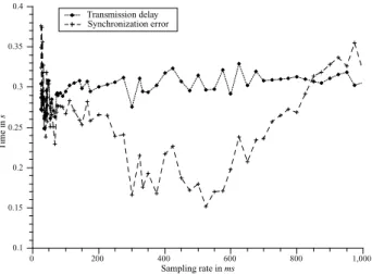
By using sampling rates between 25 and 1000 mil-liseconds, we show that the synchronization error can be bounded according to the transmission delay as shown in Figure 11.
4.2.1 Analysis of the results
Based on the ES-LM, the data alignment is performed in the intermediate nodes while the streams are propagated through the network. In our case the data alignment is achieved by ensuring at each intermediate node the syn-chronization error εj(e∗α,e
∗
ρ) is bounded by the transmission
delay for a pair of endpoints e∗αand e ∗
ρ. This means that the
execution of the send events of such pair of endpoints take place at most at εj(e∗α,e
∗
T ime in s 0.15 0.2 0.25 0.3 0.35 0.4 Transmission delay Synchronization error 0.1 Sampling rate in ms 0 200 400 600 800 1,000
Figure 11: Difference between the synchronization error and the transmission delay.
the another. This result is achieved as follows. When pj
lo-cally constructs an event-streaming, such event-streaming is the output of the alignment of two or more local-streams according to the causal relations established by ES-LM. In such event-streaming, a pair of endpoints (e∗α,e
∗ ρ) is
re-lated at pj as shown in Figure 10. When such endpoints
are retransmitted/propagated to another node (final or in-termediate), and because they have the same source, their transmission delays will be affected by the same network conditions and therefore the synchronization error remains bounded according to the transmission delay of the current hop. This phenomenon is quite similar to the relative veloc-ity between two physical objects.
With respect to why the average synchronization error is bounded between sampling rates of 75 ms to 830 ms we present the following analysis (see Figure 11). The syn-chronization error cannot be bounded lower than 75 ms be-cause a faster sampling rate be-causes a greater saturation in communication channels and indeterminism of the trans-mission delay. The latter is mainly due to the signal-to-noise ratio (SNR) as well as to the medium access con-tention. On the other hand, the synchronization error can-not be bounded when the sampling rates are greater than 830 ms by our solution since the temporal distance between two consecutive local samples at a process pjis much larger
than the maximum transmission delay of the current hop.
5
Conclusions
A temporal alignment model for data streams in WSNs called event-streaming logical mapping (ES-LM) has been presented. One original aspect of our model is that the data alignment is performed without using synchronized clocks, global references, centralized schemes or additional synchronization signals. This was achieved by translating temporal dependencies based on a time-line to causal de-pendencies among streams. The ES-LM model constructs a virtual time-line by arranging the transmitted data into
causally-ordered sets of events. In terms of the problem of temporal data alignment, it was proven that each ordered set of events determines a specific and unique time slot. An instantiation of the model was simulated over a sen-sor network with multi-hop communication. The simula-tion results show that the synchronizasimula-tion error is bounded according to the transmission delay.
A
Conflict of interests
The only funding source for this work is mentioned in the acknowledgment section of the paper. The authors declare that there is no conflict of interests regarding the publication of this article.
B
Acknowledgments
Jose Roberto Perez Cruz would like to thank to the Council of Science and Technology (CONACYT) of Mexico for the doctoral scholarship with which his studies were supported.
References
[1] Ian F. Akyildiz, Tommaso Melodia, and Kaushik R. Chowdhury. A survey on wireless multimedia sensor networks. Computer Networks, 51(4):921–960, 2007. [2] James F. Allen. Maintaining knowledge about tempo-ral intervals. Communications of the ACM, 26:832– 843, November 1983.
[3] Jacques M. Bahi, Arnaud Giersch, and Abdallah Makhoul. A scalable fault tolerant diffusion scheme for data fusion in sensor networks. In Proceedings of
the 3rd international conference on Scalable informa-tion systems, InfoScale ’08, pages 10:1–10:5, ICST, Brussels, Belgium, Belgium, 2008. ICST (Institute for Computer Sciences, Social-Informatics and Telecom-munications Engineering).
[4] Eva Besada-Portas, Jose A. Lopez-Orozco, Juan Be-sada, and Jesus M. de la Cruz. Multisensor fu-sion for linear control systems with asynchronous, out-of-sequence and erroneous data. Automatica, 47(7):1399–1408, July 2011.
[5] A. Boulis. Castalia: A simulator for wireless sensor networks. http://castalia.research.nicta.com.au/, June 2013.
[6] Punit Chandra and Ajay D. Kshemkalyani. Causality-based predicate detection across space and time. IEEE
Trans. Comput., 54:1438–1453, November 2005. [7] Colin J. Fidge. Timestamps in Message-Passing
Sys-tems That Preserve the Partial Ordering. In
Proceed-ings of the 11th Australian Computer Science Confer-ence (ACSC’88), pages 56–66, 1988.
[8] Mingyan Gao, Xiaoyan Yang, Ramesh Jain, and Beng Chin Ooi. Spatio-temporal event stream pro-cessing in multimedia communication systems. In
Proceedings of the 22nd international conference on Scientific and statistical database management, SS-DBM’10, pages 602–620, Berlin, Heidelberg, 2010. Springer-Verlag.
[9] David L. Hall and Sonya A. H. McMullen.
Mathemat-ical Techniques in Multisensor Data Fusion (Artech House Information Warfare Library). Artech House, Inc., Norwood, MA, USA, 2004.
[10] Ajay D. Kshemkalyani. Predicate detection using event streams in ubiquitous environments. In
Pro-ceedings of the EUC 2005 Workshops: UISW, NCUS, SecUbiq, USN, and TAUES, pages 807–816, Na-gasaki, Japan, 2005. Springer Berlin / Heidelberg. [11] Ajay D. Kshemkalyani and Mukesh Singhal.
Dis-tributed Computing: Principles, Algorithms, and Sys-tems. Cambridge University Press, New York, NY, USA, 2008.
[12] Leslie Lamport. Time, clocks, and the ordering of events in a distributed system. Commun. ACM, 21(7):558–565, 1978.
[13] Leslie Lamport. On interprocess communication. part ı: Basic formalism,. Distributed Computing, 1(2):77– 85, 1986.
[14] Guo-Liang Lee and Chi-Sheng Shih. Clock free data streams alignment for sensor networks. In 13th IEEE
International Conference on Embedded and Real-Time Computing Systems and Applications, 2007. RTCSA 2007, pages 355–362, 2007.
[15] Marc B. Vilain. A System for Reasoning about Time. In 2nd. (US) National Conference on Artificial
Intelli-gence, pages 197–201. MIT Press, 1982.
[16] Friedemann Mattern. Virtual Time and Global States in Distributed Systems. In Proc. Int. Workshop on
Parallel and Distributed Algorithms, pages 215–226, Gers, France, 1988. North-Holland.
[17] Jose Roberto Perez Cruz, Saul Eduardo Pomares Her-nandez, and Enrique Munoz de Cote. Data align-ment for data fusion in wireless multimedia sensor networks based on M2M. KSII Transactions on
In-ternet and Information Systems, 6(1):229–240, 2012. [18] Sean Reilly. Multi-event handlers for sensor-driven
ubiquitous computing applications. In Proceedings of
the 2009 IEEE International Conference on Pervasive Computing and Communications, pages 1–2, Wash-ington, DC, USA, 2009. IEEE Computer Society. [19] Saul Pomares Hernandez, Jean Fanchon, and Khalil
Drira. The immediate dependency relation: an
optimal way to ensure causal group communica-tion. In Annual Review Of Scalable Computing,
Edi-tions World Scientific, Series On Scalable Computing, pages 61–79, 2004.
[20] Saul Pomares Hernandez, Jorge Estudillo Ramirez, Luis A. Morales Rosales, and Gustavo Rodr´ıguez G´omez. Logical mapping: An intermedia synchro-nization model for multimedia distributed systems.
Journal of Multimedia, 3(5):33–41, 2008.
[21] Kenichi Shimamura, Katsuya Tanaka, and Makoto Takizawa. Group communication protocol for multi-media applications. In Proceedings of the 2001
Inter-national Conference on Computer Networks and Mo-bile Computing (ICCNMC’01), ICCNMC ’01, pages 303–308, Washington, DC, USA, 2001. IEEE Com-puter Society.