HAL Id: inria-00432810
https://hal.inria.fr/inria-00432810v2
Submitted on 24 Jan 2012HAL is a multi-disciplinary open access archive for the deposit and dissemination of sci-entific research documents, whether they are pub-lished or not. The documents may come from
L’archive ouverte pluridisciplinaire HAL, est destinée au dépôt et à la diffusion de documents scientifiques de niveau recherche, publiés ou non, émanant des établissements d’enseignement et de
A Case Study in Formalizing Projective Geometry in
Coq: Desargues Theorem
Nicolas Magaud, Julien Narboux, Pascal Schreck
To cite this version:
Nicolas Magaud, Julien Narboux, Pascal Schreck. A Case Study in Formalizing Projective Geometry in Coq: Desargues Theorem. Computational Geometry, Elsevier, 2012, Special Issue on geometric reasoning, 45 (8), pp.406-424. �10.1016/j.comgeo.2010.06.004�. �inria-00432810v2�
A Case Study in Formalizing Projective Geometry in
Coq: Desargues Theorem
∗Nicolas Magaud, Julien Narboux, Pascal Schreck Universit´e de Strasbourg - Laboratoire des Sciences de l’Image, de l’Informatique et de la T´el´ed´etection (LSIIT, UMR 7005 CNRS-UDS)
Pˆole API, Boulevard S´ebastien Brant, BP 10413, 67412 Illkirch, France {magaud,narboux,schreck}@lsiit-cnrs.unistra.fr
Abstract
Formalizing geometry theorems in a proof assistant like Coq is challeng-ing. As emphasized in the literature, the non-degeneracy conditions lead to long technical proofs. In addition, when considering higher-dimensions, the amount of incidence relations (e.g. point-line, point-plane, line-plane) induce numerous technical lemmas. In this article, we investigate formalizing projec-tive plane geometry as well as projecprojec-tive space geometry. We mainly focus on one of the fundamental properties of the projective space, namely Desargues property. We formally prove that it is independent of projective plane geom-etry axioms but can be derived from Pappus property in a two-dimensional setting. Regarding at least three dimensional projective geometry, we present an original approach based on the notion of rank which allows to describe incidence and non-incidence relations such as equality, collinearity and copla-narity homogeneously. This approach allows to carry out proofs in a more systematic way and was successfully used to fairly easily formalize Desargues theorem in Coq. This illustrates the power and efficiency of our approach (using only ranks) to prove properties of the projective space.
Key words: formalization, Desargues, rank, projective geometry, Coq,
Hessenberg theorem, Hexamys
1. Introduction
This article deals with formalizing projective geometry in the Coq proof assistant [1, 7] and studies Desargues property both in the plane and in an at least three dimensional setting (noted ≥ 3-dimensional). In the plane, proofs are constructed in a traditional way using points and lines. However, in a ≥3-dimensional space, we use the concept of rank to formally prove Desargues theorem (in Coq). In the longer term, the underlying objective of the presented work consists in designing a formal geometry prover able to handle the non-degeneracy conditions, and especially in geometric constraint solving [14, 16].
We choose to focus on projective geometry which is a simple but powerful enough setting to express arbitrarily complex problems as shown in [20]. Moreover, in 3D (or higher), proofs become much more difficult than in 2D: first, Desargues property becomes a theorem and consequently all the projective spaces arise from a division ring; second incidence geometry has to deal not only with points and lines, but also with planes or, more generally, flats; third there is a combinatorial explosion of cases.
For projective plane geometry, we use a traditional approach dealing with points, lines and an incidence relation to formally prove the independence of Desargues property. We then formalize Pappus property as well as hexamys in order to prove Hessenberg theorem, which states that Pappus property entails Desargues property in projective plane geometry.
When it comes to ≥3-dimensional projective geometry , we propose to reuse the concept of rank. We aim at showing that this mathematical concept is well-suited to formalize the foundations of incidence geometry in a proof assistant. Ranks provide a generic way to describe incidence relations and it allows us to express non-degeneracy conditions nicely. Informally, ranks allow to distinguish between equal/non-equal points, collinear/non-collinear points, coplanar/non-coplanar points, etc. We validate this approach by sucessfully carrying out a mechanized proof (using only ranks) of Desargues theorem which is one of the fundamental theorems of the projective space.
We mechanize the proofs using the Coq proof assistant which implements a higher order intuitionistic logic based on type theory. In such a proof as-sistant, every step of reasoning is proposed by the user (in the form of a
tactic) but then checked by the system. It dramatically increases the
relia-bility of the proofs compared to paper-and-pencil proofs. In addition, during the development process, the ability to change the axiom system easily is
very convenient. Proofs can be automatically rechecked by the system and changes only require minor rewriting of the proofs. However, formal proofs tend to be more technical to write, not leaving out a single piece of details.
Therefore, in our development, we had to design some efficient proof techniques to deal with points and lines in the plane as well as with matro¨ıd and rank properties when the dimension n of the considered space is greater than 2. In addition, we believe a full scale automation is out of scope, but many small-scale simple automated tactics make writing formal proofs in Coq more tractable.
Related work Proof assistants have already been used in the context of
geometry. Numerous papers have emphasized the importance of the problem of degenerate cases in formal geometry [9, 13, 19, 24]. Brandt and Schnei-der studied how to handle degenerate cases for the orientation predicates in computational geometry using three valued logic [3]. Bezem and Hen-dricks formalized Hessenberg’s theorem in Coq [2]. Guilhot has formalized in Coq a proof of Desargues theorem in affine geometry [13]. Narboux has formalized in Coq the area method of Chou, Gao and Zhang [6, 15, 23] and applied it to obtain a proof of Desargues theorem in affine geometry. Kusak has formalized in Mizar Desargues theorem in the Fanoian projective ≥3-dimensional space [17]. The assumption that the space is Fanoian makes the theorem more specialized than ours. We also carried out some preliminary work on formalizing projective plane geometry in Coq [18]. Finally, the idea of proving projective space theorems with ranks is suggested by Michelucci and Schreck in [21].
Outline of the paper The paper is organized as follows. In section 2, we
present the axioms for projective geometry and we give an overview of our Coq formalization. In section 3, we explain Desargues property and why it is a fundamental property of projective geometry. Section 4 investigates the role of Desargues property in the case of the generic 2D projective plane and its links with Pappus property through the notion of Hexamys. Section 5 introduces ranks and the associated axiom system for projective space geom-etry, which is then used to formally prove in Coq that Desargues property holds in ≥3-dimensional projective space.
2. Axiom Systems of Projective Geometry
Projective geometry is a general setting in the hierarchy of geometries which assumes that two lines in a plane always meet [4, 8]. We first assume
that we have two kinds of objects (points and lines). Planes are not basic objects in this axiom system, but are defined within the theory. We then consider a relation (∈) between elements of these two sets.
2.1. Axiom System for Projective Plane Geometry
The axiom system for projective plane geometry consists of very few axioms linking abstact points and lines of a plane. Informally, these axioms capture the facts that two different points define one line and two different lines define one point. Moreover, each line contains at least three points and there are at least two lines in the plane. Formally, we have the following five axioms:
Line-Existence ∀A B : P oint, ∃l : Line, A ∈ l ∧ B ∈ l Point-Existence ∀l m : Line, ∃A : P oint, A ∈ l ∧ A ∈ m Uniqueness ∀A B : P oint, ∀l m : Line,
A ∈ l ∧ B ∈ l ∧ A ∈ m ∧ B ∈ m ⇒ A = B ∨ l = m Three-Points ∀l : Line, ∃ABC : P oint,
A 6= B ∧ B 6= C ∧ A 6= C ∧ A ∈ l ∧ B ∈ l ∧ C ∈ l Lower-Dimension-2 ∃l : Line, ∃m : Line, l 6= m
The axiom Lower-Dimension-2 prevents a single line from being a model, i.e. it ensures we actually describe a two dimensional projective space.
2.2. Axiom System for Projective Space Geometry
Several axioms remains the same when we consider an ≥3-dimensional space. The required axioms for projective ≥3-dimensional space are listed below:
Line-Existence ∀A B : P oint, ∃l : Line, A ∈ l ∧ B ∈ l
Pasch
∀A B C D : P oint, ∀lABlCDlAClBD: Line,
A 6= B ∧ A 6= C ∧ A 6= D ∧ B 6= C ∧ B 6= D ∧ C 6= D∧ A ∈ lAB ∧ B ∈ lAB ∧ C ∈ lCD ∧ D ∈ lCD∧
A ∈ lAC ∧ C ∈ lAC∧ B ∈ lBD∧ D ∈ lBD∧
(∃I : P oint, I ∈ lAB ∧ I ∈ lCD) ⇒
b A b B b C b D b I b J
Figure 1: Pasch’s axiom
Uniqueness ∀A B : P oint, ∀l m : Line,
A ∈ l ∧ B ∈ l ∧ A ∈ m ∧ B ∈ m ⇒ A = B ∨ l = m Three-Points ∀l : Line, ∃ABC : P oint,
A 6= B ∧ B 6= C ∧ A 6= C ∧ A ∈ l ∧ B ∈ l ∧ C ∈ l Lower-Dimension-3 ∃l m : Line, ∀p : P oint, p 6∈ l ∨ p 6∈ m
The Point-Existence axiom is replaced by Pasch axiom. Indeed we need to ensure that two lines always meet only if co-planar. Axiom Lower-Dimension-3 ensures that there exists two lines which do not meet.
2.3. Formalization in Coq
Implementing both axiom systems in the Coq proof assistant is straight-forward. Figure 2 presents the formalization of the projective space in Coq. We denote the predicate ∈ using Incid. To enhance modularity we make use of the module system of Coq.
The main difference between the formalization and the axiom system shown above relies on the fact that we need to be carefull about the equality relations and decidability issues. In addition, the equality on points (noted DecPoints.eq) and lines (noted line_eq) are parameters of our theory. As the underlying logic of the Coq system is intuitionistic, we have to state explicitly which predicates are assumed to be decidable. We assume that we have a set of points with a decidable equality : DecPoints is a instance of a DecidableType:
Module Type ProjectiveSpaceOrHigher (DecPoints: DecidableType). Definition Point := DecPoints.t.
Parameter Line : Type.
Parameter line_eq : Line -> Line -> Prop.
Axiom line_eq_sym : forall l m, line_eq l m -> line_eq m l. Axiom line_eq_trans : forall l m n,
line_eq l m -> line_eq m n -> line_eq l n. Axiom line_eq_refl : forall l, line_eq l l. Parameter Incid : Point -> Line -> Prop.
Axiom incid_dec : forall (A:Point)(l:Line),{Incid A l}+{~Incid A l}. Axiom line_existence : forall A B : Point,
{l : Line | Incid A l /\ Incid B l}.
Axiom pasch : forall A B C D:Point, forall lAB lCD lAC lBD :Line, dist4 A B C D ->
Incid A lAB/\Incid B lAB -> Incid C lCD/\Incid D lCD -> Incid A lAC/\Incid C lAC -> Incid B lBD/\Incid D lBD -> (exists I:Point, (Incid I lAB /\ Incid I lCD)) ->
exists J:Point, (Incid J lAC /\ Incid J lBD). Axiom uniqueness : forall (A B :Point)(l1 l2:Line),
Incid A l1 -> Incid B l1 -> Incid A l2 -> Incid B l2 -> DecPoints.eq A B \/ line_eq l1 l2.
Axiom three_points :
forall l:Line,exists A:Point, exists B:Point, exists C:Point, dist3 A B C /\ Incid A l /\ Incid B l /\ Incid C l.
Axiom lower_dimension_3 : exists l:Line, exists m:Line, forall p:Point, ~Incid p l \/ ~Incid p m.
End ProjectiveSpaceOrHigher.
Module Type DecidableType. Parameter t : Set.
Parameter eq : t -> t -> Prop.
Axiom eq_refl : forall x : t, eq x x.
Axiom eq_sym : forall x y : t, eq x y -> eq y x. Axiom eq_trans : forall x y z : t,
eq x y -> eq y z -> eq x z. Parameter eq_dec : forall x y : t,
{ eq x y } + { ~ eq x y }. End DecidableType.
The notation {eq x y}+{~ eq x y} means that we must know construc-tively that either x = y or x 6= y. As expressed by the axiom incid_dec we also assume the decidability of incidence. In Coq syntax /\, \/ and ~ stands respectively for logic conjunction, disjunction and negation. The no-tation {l : Line | Incid A l /\ Incid B l} expresses that there exists a line l going through A and B.
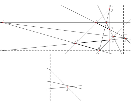
3. Desargues Property
Desargues property is among the most fundamental properties of projec-tive geometry, since in the projecprojec-tive space Desargues property becomes a theorem. Let’s first recall Desargues statement in projective geometry. De-sargues property states that:
Let E be a projective space and A,B,C,A′,B′,C′ be points in E, if the
three lines joining the corresponding vertices of triangles ABC and A′B′C′
all meet in a point O, then the three intersections of pairs of corresponding sides α, β and γ lie on a line.
b A b B b C b O b C’ b A’ b B’ b b b β γ α
If E is of dimension two, Desargues property is independent from all the projective plane geometry axioms. If E is at least of dimension three, Desargues property is a theorem.
Even though it can be expressed, it is not provable when E is a plane. Indeed in the 2D case, some projective planes are Desarguesian, for instance Fano’s plane, while other planes are not, for instance Moulton plane. The next section investigates the role of Desargues property in projective planes.
4. Desargues Property in the Projective Plane
Projective Plane Geometry as defined above is incomplete. Indeed, De-sargues statement does not hold in every model. We show on the one hand, that Desargues property is consistent with the axioms of projective geometry and, on the other hand, that it is independent of them. First we formalize a proof that it is true in a particular model of projective plane geometry (Fano’s plane) and then a proof that in another particular model (Moulton’s plane) it is false. This shows the independence of Desargues theorem from the axioms of projective plane geometry, which can be regarded as the start-ing point of non-desarguesian geometry [5]. Finally we formalize the proof of Hessenberg’s theorem which demonstrates that in every projective plane in which Pappus property holds, Desargues property holds as well.
4.1. Consistency of Desargues Property with Axioms for Projective Plane Geometry
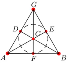
Fano’s plane is the model of projective plane geometry with the least number of points and lines: 7 each. The incidence relation is illustrated by
b A bB b b G bE b F b D bC
Figure 3: Fano’s plane
the figure. In the figure, points are simply represented by points, whereas lines are represented by six segments and a circle (DEF ). One can verify that the axioms of projective plane geometry (see Section 2.1) hold as shown in [18].
At first sight, proving Desargues property in Fano’s plane seems to be straightforward to achieve by case analysis on the 7 points and 7 lines. How-ever, this requires handling numerous cases2
including many configurations which contradict the hypotheses.
To formalize the property, we make use of two kinds of symmetries: a symmetry of the theory and a symmetry of the statement.
Symmetry of the statement
We first study the special case desargues_from_A_specialized where the point O of Desargues configuration corresponds to A, and the line OA corresponds to ADG, OB to CAE and OC to ABF .
The predicate on line A B C l states that the three points A, B and C lie on the line l.
Lemma Desargues_from_A_specialized : forall P Q R P’ Q’ R’ alpha beta gamma
lPQ lPR lQR lP’Q’ lP’R’ lQ’R’,
((on_line P Q gamma lPQ) /\ (on_line P’ Q’ gamma lP’Q’)) /\ ((on_line P R beta lPR) /\ (on_line P’ R’ beta lP’R’)) /\ ((on_line Q R alpha lQR) /\ (on_line Q’ R’ alpha lQ’R’)) /\ ((on_line A P P’ ADG) /\
(on_line A Q Q’ CAE) /\
2
The most na¨ıve approach would consider 77
cases and even with careful analysis it remains untractable to prove all the cases without considering symmetries.
(on_line A R R’ ABF)) /\
~collinear A P Q /\ ~collinear A P R /\ ~collinear A Q R /\ ~collinear P Q R /\ ~collinear P’ Q’ R’ /\
((P<>P’)\/(Q<>Q’)\/(R<>R’)) -> collinear alpha beta gamma.
Then as Desargues statement is symmetric by permutation of the three lines which intersect in O, we can formalize a proof of slightly more general lemma desargues_from_A where the point O of Desargues configuration still corresponds to A but the three lines (lP,lQ and lR) intersecting in O are universally quantified.
Lemma Desargues_from_A :
forall P Q R P’ Q’ R’ alpha beta gamma lP lQ lR lPQ lPR lQR lP’Q’ lP’R’ lQ’R’,
((on_line P Q gamma lPQ) /\ (on_line P’ Q’ gamma lP’Q’)) /\ ((on_line P R beta lPR) /\ (on_line P’ R’ beta lP’R’)) /\ ((on_line Q R alpha lQR) /\ (on_line Q’ R’ alpha lQ’R’)) /\ ((on_line A P P’ lP) /\
(on_line A Q Q’ lQ) /\ (on_line A R R’ lR)) /\
~collinear A P Q /\ ~collinear A P R /\ ~collinear A Q R /\ ~collinear P Q R /\ ~collinear P’ Q’ R’ /\
((P<>P’)\/(Q<>Q’)\/(R<>R’)) -> collinear alpha beta gamma.
Symmetry of the theory
The theory of Fano’s plane is invariant by permutation of points. It means that, even if it is not obvious from Figure 3, all the points plays the same role: if (A, B, C, D, E, F, G) is a Fano’s plane then (B, C, D, F, E, G, A) is one as well. We formalize this by building a functor from Fano’s theory to itself which permutes the points (Figure 4).
Using this functor and desargues_from_A, we show that Desargues prop-erty holds for any choice for O among the 7 points of the plane. Intuitively, this functor shows that the problem is symmetric and hence that the proof can assume without loss of generality that O = A.
Module swapf3 (M:fano_plane) : fano_plane with [...]
Definition Point:=M.Point.
Definition A:=M.B. Definition B:=M.E. Definition C:=M.D. Definition D:=M.F. Definition E:=M.C. Definition F:=M.G. Definition G:=M.A.
[...]
Definition ABF:=M.BEG. Definition BCD:=M.DEF. Definition CAE:=M.BCD. Definition ADG:=M.ABF. Definition BEG:=M.CAE. Definition CFG:=M.ADG. Definition DEF:=M.CFG.
[...]
End swapf3.
4.2. Independence of Desargues Property from the Axioms for Projective Plane Geometry
We now consider a particular model of projective plane geometry, namely Moulton plane and show that Desargues property does not hold in this model.
4.2.1. Moulton plane and its projective counterpart
Moulton plane [22] is an affine plane in which lines with a negative slope are bent (i.e. the slope is doubled) when they cross the y-axis. It can be easily extended into a projective plane.
Moulton plane is an incidence structure which consists in a set of points P , a set of lines L, and an incidence relation between elements of P and elements of L. Points are represented by couples (x, y) ∈ R2
. Lines are represented by couples (m, b) ∈ (R ∪ ∞) × R (where m is the slope - ∞ for vertical lines - and b the y-intercept). The incidence relation is defined as follows: (x, y) ∈ (m, b) ⇐⇒ x = b if m = ∞ y = mx + b if m ≥ 0 y = mx + b if m ≤ 0, x ≤ 0 y = 2mx + b if m ≤ 0, x ≥ 0.
This incidence structure verifies the properties of an affine plane. It can be turned into a projective plane through the following process.
• We extend P with points at the infinite (one direction point for each possible slope, including the vertical one); therefore P is (R × R) ∪ (R ∪ ∞).
• We extend the set L of affine lines with a new one which connects all points at the infinite; therefore L is ((R ∪ ∞) × R) ∪ ∞.
• We finally extend the incidence relation in order to have all direction points and only them incident to the infinite line. We also extend each affine line with a direction point (the one bearing its slope).
This construction leads to a projective plane. The whole process is formally described in Coq and we formalize in Coq (see [18] for details) that all the axioms of projective plane geometry presented in section 2.1 hold. Most proofs on real numbers rely on using Gr¨obner basis computation in Coq [12].
4.2.2. A counter-model for Desargues Property
We build a special configuration of Desargues for which the property does not hold. This can be achieved in an algebraic way using only coordinates and equations for lines. We first present it that way and then show why Desargues property does not hold for our configuration.
Let’s consider seven points: O(−4, 12), A(−8, 8), B(−5, 8), C(−4, 6), A′(−14, 2), B′(−7, 0) and C′(−4, 3). We then build the points α(−3, 4),
β(6/11, 38/11) and γ(−35, 8) which are respectively at the intersection of (BC) and (B′C′), (AC) and (A′C′) and (AB) and (A′B′). Then we can
check using automated procedures performing symbolic computation on real numbers (especially the fourier tactic [7]) that there exists no line in Moulton plane which is incident to these 3 points α, β and γ. The intuitive idea of this counter-example is to build a configuration where:
• all points except β are in the left hand side plane and
• the lines (AC) and (A′C′) which define β have slopes of opposite signs.
Overall Desargues property does not hold in this configuration because only some of the lines are bent. Especially, of the two lines used to build β, one of them is a straight line (A′C′) and the other one (AC) is bent. That
is what prevents the three points α, β and γ from being on the same line. Proofs of these lemmas illustrate how combining automated and
interac-tive theorem proving can be successful.
4.3. Hessenberg’s Theorem: Pappus Property Implies Desargues Property
In this section, we describe our formalization of Hessenberg’s theorem stating that Pappus axiom implies that Desargues property holds in the projective plane. The proof we formalize use the concept of hexamys (mystic
hexagrams as named by Pascal) and popularized by [25]. We formalized the
proof given in [21] and extend it to deal with some degenerate cases. First, we need to state the Pappus property.
4.3.1. Pappus Property
We say that a plane enjoys Pappus property when: Definition pappus_weak :=
forall A B C A’ B’ C’ P Q R, Col A B C -> Col A’ B’ C’ ->
b b b b b b b b b b A B C A’ B’ C’ O α γ β b b b b b b b b b b β
Figure 5: Counter example to Desargues theorem in Moulton plane
b A b B b C b A’ b B’ b C’ b P b Q b R
all_distinct_6 A B C A’ B’ C’ -> is_on_proper_inter P A B’ A’ B -> is_on_proper_inter Q B C’ B’ C -> is_on_proper_inter R A C’ A’ C -> Col P Q R.
The property is_on_proper_inter P A B’ A’ B means that the lines AB′ and A′B are well defined and not parallel and P is at the intersection.
This definition of Pappus configuration assumes that the six points are dis-tinct and that the intersections are all well defined. This also implies that the lines AB and A′B′ are distinct. This definition captures a general
con-figuration as shown in Figure 6 without any particular case. But, in field of formal proofs, we must be careful about degenerate cases. Fortunately in the context of projective geometry, the weak version of Pappus property as stated above is also equivalent to this stronger version which assumes that either all the intersections are well defined or the six points (A,B,C,A′,B′,C′)
are distinct:
Definition pappus_strong := forall A B C A’ B’ C’ P Q R, (all_distinct_6 A B C A’ B’ C’ \/
(line A B’ <> line A’ B /\ A<>B’ /\ A’<>B /\ line B C’ <> line B’ C /\ B<>C’ /\ B’<>C /\ line A C’ <> line A’ C /\ A<>C’ /\ A’<>C) ) -> Col A B C -> Col A’ B’ C’ ->
is_on_inter P A B’ A’ B -> is_on_inter Q B C’ B’ C -> is_on_inter R A C’ A’ C -> Col P Q R.
4.3.2. Mystic hexagram
We say that a hexagon is a hexamy if the three intersections of the op-posite sides of the hexagon are collinear.
Definition is_hexamy A B C D E F := all_distinct_6 A B C D E F /\
let P:= inter (line B C) (line E F) in let Q:= inter (line C D) (line F A) in let R:= inter (line A B) (line D E) in Col P Q R.
It is easy to show that every circular permutation of a hexamy is also a hexamy.
Lemma hexamy_rot_left : forall A B C D E F,
is_hexamy A B C D E F -> is_hexamy B C D E F A.
We say that a plane enjoys the hexamy property if every permutation of a hexamy is also a hexamy. As circular permuations of hexamys are hexamys, we just need to assume that if (A, B, C, D, E, F ) is a hexamy, then (B, A, C, D, E, F ) is also a hexamy:
Definition hexamy_prop := forall A B C D E F, is_hexamy A B C D E F -> is_hexamy B A C D E F.
We can show that the hexamy property and Pappus property are equiv-alent.
Lemma 1. Pappus property implies hexamy property.
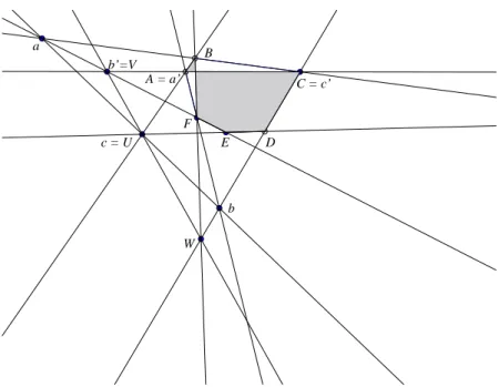
Proof. Assuming Pappus property, we need to show that if (A, B, C, D, E, F ) is a hexamy so is (B, A, C, D, E, F ). Let U,V and W be the intersections of AB and DE, AC and EF , and CD and BF respectively. We need to show that U, V and W are collinear. Let a, b and c be the intersections of BC and EF , CD and F A, and AB and DE respectively (we have c = U). As (A, B, C, D, E, F ) is a hexamy, a, b and c are collinear. Let b′ be the
intersection of EF and AC (we have b′ = V ). We note a′ ≡ A and c′ ≡ C.
a′, b′ and c′ are collinear because b′ is on line AC. Using Pappus
prop-erty, it holds that ab′ ∩ a′b, ac′ ∩ a′c and bc′ ∩ b′c are collinear. We have
ab′∩ a′b = F since a′b = AF and ab′ = EF . Similarly, we have ac′∩ a′c = B.
Hence the third point bc′ ∩ b′c is on BF . Hence, as bc′ = CD, we have
bc′ ∩ b′c = CD ∩ BF = W . The last equality says that W ∈ b′c but since
b′ = V and c = U, the collinearity of U, V and W holds.
Lemma 2. Hexamy property implies Pappus property.
Proof. When (A,B,C,A′,B′,C′) is a Pappus configuration, it is easy to show
that it is also a hexamy because the intersections of AB ∩A′B′ and BC ∩B′C′
are equal since the points A,B and C and A′, B′ and C′ are collinear. Using
the hexamy property we can show that (A,B′,C,A′,B,C′) is also a hexamy.
b C = c’ a D B b’=V c = U W F E A = a’
Figure 7: Pappus property implies hexamy property
4.3.3. Hessenberg theorem
Lemma 3. Hexamy property implies Desargues property
Proof. Recall that A′B′C′ is a Cevian triangle of ABC if A′ ∈ BC, B′ ∈
AC, C′ ∈ AB and the lines AA′, BB′and CC′are concurrent. We distinguish
two cases, either A′B′C′ is a Cevian triangle of ABC or not.
b A b B b C b O b C’ b A’ b B’ b b P Q b b b β γ α
First, we assume that A′B′C′ is not a Cevian triangle of ABC. By
hy-pothesis, points O, A and A′ are collinear. Similarly, O, B and B′ are
collinear and O, C, C′ are collinear. We want to prove that α, β and γ
are collinear, where α = BC ∩ B′C′, β = AC ∩ A′C′ and γ = AB ∩ A′B′.
The auxiliary points: P = A′B′ ∩ BC, Q = AB ∩ B′C′ are needed. Now
(A, A′, P, C, C′, Q) is a hexamy since its three opposite sides cut
respec-tively in points O, B′ and B which are collinear by hypothesis. Thus
(A, Q, C′, A′, P, C) is a hexamy as well, the opposite sides cut respectively in
α, β and γ, hence they are collinear.
b b b A B C b O b b C’ A’ b B’ b b b b I L N M b b b β γ α = α1=α2
Second, we assume that A′B′C′ is a Cevian triangle of ABC. We have to
prove that α, β and γ are collinear where α = BC ∩B′C′, β = AC ∩A′C′ and
γ = AB ∩ A′B′. We introduce α
1 = βγ ∩ BC and α2 = βγ ∩ B′C′: now we
have to prove that α1 = α2. Auxiliary intersection points are I = OB ∩ βγ,
L = A′C′∩ AI, N = AB ∩ LB′ and M = AL ∩ CC′ (it can be shown that
these points are well defined). The end of the proof implicitely assumes that L 6= A′. If L = A′ we construct a proof similar to this one but using a
permutation of the statement, if L = B′ we permute again the statement, it
can not be the case that L = A′ = B′ = C′.
Since points L, N and B′ are collinear, (A′, L, B′, I, A, γ) is a hexamy, so
is (A′, A, γ, I, B′, L), and hence O, N and β are collinear. With the
sec-ond hexamys, (C, B, A, O, I, β) which gives by permutation (C, O, β, I, A, B), we prove that α1, M and N are collinear. A third hexamys is used to
(C′, O, β, I, L, B′). Thus the lines MN and βγ have two points in common:
α1 and α2. From the uniqueness axiom, it holds that :
• either the lines are equal but then the configuration degenerates and all points belong to the same line;
• or α1 = α2 and therefore α, β and γ are collinear.
Corollary 1 (Hessenberg). Pappus property implies Desargues property
Proof. Immediate using lemmas 1 and 3.
The formal proofs corresponding to the theorems described in this section still heavily require user-interaction and lack automation. The amount of case distinctions required in formal proofs makes them difficult to handle.
4.4. Dealing with Non-degeneracy Conditions: Using Tactics
In this section, we describe a tactic whose implementation is simple but which is still powerfull enough to shorten the proofs about degenerate cases. When we know that two points are equal, we can propagate this knowledge. The tactic performs repeated applications of the uniqueness axiom. It pro-ceeds by searching for pattern matching the hypotheses of the two following lemmas which are easy consequences of the uniqueness axiom.
A ∈ l ∧ B ∈ l
A ∈ m ∧ B ∈ m ∧ A 6= B ⇒ l = m A ∈ l ∧ B ∈ l
A ∈ m ∧ B ∈ m ∧ l 6= m ⇒ A = B It is implemented using Coq tactic language as follows: Ltac apply_unicity := match goal with
H1: ?A <> ?B,
H2: ?Incid ?A ?l, H3: ?Incid ?B ?l,
H4: ?Incid ?A ?m, H5: ?Incid ?B ?m |- _ => let id:= fresh in assert (id: l=m);
try apply (uniq.a1_unique A B l m H1 H2 H3 H4 H5); subst l
| H1: ?l <> ?m,
H4: ?Incid ?B ?l, H5: ?Incid ?B ?m |- _ => let id:= fresh in assert (id: A=B);
try apply (uniq.a2_unique l m A B H1 H2 H3 H4 H5); subst A
end.
Ltac collapse := progress (repeat (apply_unicity; CleanDuplicatedHyps)).
For example, if we know that A, B, C, A′, B′ and C′ are all distinct and
that they form a Pappus configuration and that the line A′B is equal to the
line AB′ then our collapse tactic infers automatically that the lines AB,
AB′, A′C, AB′, BC′, AC′, B′C are all equal. This allows to conclude easily
that Pappus theorem holds trivially in this special case (when line A′B is
equal to line AB′).
5. Desargues Property in Projective Space
In this section, we switch from projective plane geometry to projective space geometry. In 2D, a single fact can have numerous representations (e.g. A ∈ BC vs. A ∈ l ∧ B ∈ l ∧ C ∈ l). In 3D and more, it is even worse because the language contains points, lines and planes and all the associated incidence relations. In section 2.2, we presented the standard axiom system for projective space geometry as a reference. But to ease the formalization in Coq, we propose an alternative axiom system based on the notion of rank. Indeed, ranks allow to deal only with points which makes proofs easier in a three dimensionnal setting because we do not handle lines and planes explicitly. This provides a homogeneous description language independent of the dimension and will make proving Desargues property in a ≥3-dimensional setting much easier.
5.1. Ranks
The concept of rank is a general notion of matroid theory. An integer function rk on E is the rank function of a matroid if and only if the following conditions are satisfied:
R1 ∀X ⊆ E, 0 ≤ rk(X) ≤ |X| (nonnegative and subcardinal) R2 ∀X Y ⊆ E, X ⊆ Y ⇒ rk(X) ≤ rk(Y ) (nondecreasing)
R3 ∀X Y ⊆ E, rk(X ∪ Y ) + rk(X ∩ Y ) ≤ rk(X) + rk(Y ) (submodular) In projective geometry, we can define a rank function on sets of points which verify the axioms above: a flat being a set of points closed by the collinear-ity relation, the rank of a set of points X is the cardinal of a smallest set generating X (see Figure 8 for some examples).
rk{A, B} = 1 A = B rk{A, B} = 2 A 6= B
rk{A, B, C} = 2 A, B, C are collinear
with at least two of them distinct rk{A, B, C} ≤ 2 A, B, C are collinear
rk{A, B, C} = 3 A, B, C are not collinear rk{A, B, C, D} = 3 A, B, C, D are co-planar,
not all collinear
rk{A, B, C, D} = 4 A, B, C, D are not co-planar rk{A, B, C, D, E} ≤ 2 A, B, C, D, E are all collinear
Figure 8: Rank statements and their geometric interpretations
Using this definition, one can show that every projective space has a matroid structure, but the converse is not true. In the next section, we introduce additional axioms to capture 3D or higher projective geometry. We shall start by introducing some lemmas about ranks to simplify the proofs.
Proof techniques using ranks. In this section we describe two proof techniques
that are simple but important to simplify formal proofs.
First, all equalities about ranks (say rk(a) = rk(b)) are usually proved in two steps: first showing that rk(a) ≤ rk(b) and then that rk(a) ≥ rk(b). Consequently, when stating a lemma, it is worth being cautious about whether the actual equality is required or if one of the two inequalities is enough to go on with the proofs. This approach allows to avoid numerous technical lemmas when carrying out the formal proofs in Coq.
Second, in the proving process, we make often use of axiom R3. For instance, if we need to prove a statement like:
rk{A, B, C, D, I} + rk{I} ≤ rk{A, B, I} + rk{C, D, I}
we could be tempted to instantiate axiom R3 with X := {A, B, I} and Y := {C, D, I}. But unfortunately, this statement is not a direct consequence of
axiom R3. For instance A may be equal to C and consequently {A, B, I} ∩ {C, D, I} = {A, I}. Determining the intersection of two finite sets of points requires to distinguish cases about the equality of these points. This leads to intricate proofs in Coq. Therefore, in the rest of this paper, we shall never consider the real set theoretical intersection but a lower approximation of the intersection (noted ⊓).
Definition 1 (Literal intersection). Let L1 and L2 be two sets of points.
By definition L1⊓ L2 is the intersection of the two sets of points considered
syntactically.
Using literal intersection we can derive a more convenient version of axiom R3 which leads to fewer case distinctions:
Lemma 4 (R3-lit).
∀X Y, rk(X ∪ Y ) + rk(X ⊓ Y ) ≤ rk(X) + rk(Y )
In Coq, it is not possible to define the literal intersection. To capture this property, we use the following lemma:
Lemma 5 (R3-alt).
∀X Y I, I ⊆ X ∩ Y ⇒ rk(X ∪ Y ) + rk(I) ≤ rk(X) + rk(Y )
This lemma will be used heavily in the next sections.
5.1.1. A rank-based axiom system
Contrary to the axiom system shown in section 2.2, we assume that we have only one kind of objects, namely points. To capture the whole projective space, we need to add some new axioms to the matroid’s ones:
Rk-Singleton ∀P : P oint, rk{P } ≥ 1
Rk-Couple ∀P Q : P oint, P 6= Q ⇒ rk{P, Q} ≥ 2 Rk-Pasch ∀A B C D, rk{A, B, C, D} ≤ 3 ⇒
∃J, rk{A, B, J} = rk{C, D, J} = 2 Rk-Three-Points ∀A B, ∃C, rk{A, B, C} = rk{B, C} = rk{A, C} = 2
Rk-Lower-Dimension ∃A B C D, rk{A, B, C, D} ≥ 4
The first two ones ensure that the rank function is not degenerate. Rk-Pasch is the translation of Rk-Pasch’s axiom: rk{A, B, C, D} ≤ 3 means these points are coplanar, thus that the two lines AB and CD intersect.
Using this axiom system we formally proved all the axioms of section 2.2. In particular, the following lemmas Rk-Uniqueness and Rk-Lower-Dimension are derivable and can be used to prove the Uniqueness and Lower-Dimension-3 axiom respectively: Lemma 6 (Rk-Uniqueness). ∀A B C D M P, rk{A, B} = 2 rk{C, D} = 2 rk{A, B, M} ≤ 2 rk{C, D, M} ≤ 2 rk{A, B, P } ≤ 2 rk{C, D, P } ≤ 2 rk{A, B, C, D} ≥ 3 ⇒ rk{M, P } = 1
Proof. Using R3-alt we have:
rk{A, B, M, P } + rk{A, B} ≤ rk{A, B, M} + rk{A, B, P }
Hence rk{A, B, M, P } = 2, similarly we can show that rk{C, D, M, P } = 2. Moreover rk{A, B, C, D, M, P } ≥ 3 as rk{A, B, C, D} ≥ 3 and {A, B, C, D} ⊆ {A, B, C, D, M, P }. Finally, using R3-alt we have:
rk{A, B, C, D, M, P } + rk{M, P } ≤ rk{A, B, M, P } + rk{C, D, M, P }
3 + rk{M, P } ≤ 2 + 2
Lemma 7 (Rk-Lower-Dimension).
∃ABCD, ∀M, rk{A, B, M} 6= 2 ∨ rk{C, D, M} 6= 2
Proof. Using axiom Rk-Lower-Dimension, we obtain A,B,C and D such that rk{A, B, C, D} = 4.
Suppose that rk{A, B, M} = 2 and rk{C, D, M} = 2. Using R3-alt we have that:
rk{A, B, C, D, M} + rk{M} ≤ rk{A, B, M} + rk{C, D, M} Hence rk{A, B, C, D, M} ≤ 3, which contradicts rk{A, B, C, D} = 4.
We can also derive a lemma which expresses concisely that for every point there exists one which is different, for every line there exists a point not on this line and for every plane there exists a point not on this plane.
We carried out this proof using an alternative axiom system for ranks. Whereas our development is based on matroid axioms R1, R2 and R3, one can prove that they are equivalent to the following set of axioms:
R1’ rk(∅) = 0
R2’ rk(X) ≤ rk(X ∪ {x}) ≤ rk(X) + 1
R3’ rk(X ∪ {y}) = rk(X ∪ {z}) = rk(X) ⇒ rk(X) = rk(X ∪ {y, z}) Using this axiom system the proof is straightforward.
Lemma 8 (Construction).
∀E, rk(E) ≤ 3 ⇒ ∃P, rk(E ∪ {P }) = rk(E) + 1 Proof. Consider E such that rk(E) ≤ 3.
Using axiom Rk-Lower-Dimension we obtain A,B,C and D such that rk{A, B, C, D} = 4. Using R2’ we know that rk(E) ≤ rk(E ∪ {A}) ≤ rk(E) + 1 and similarly for B,C and D. Suppose that rk(E ∪ {A}) = rk(E ∪ {B}) = rk(E ∪ {C}) = rk(E ∪ {D}) = rk(E), then we would obtain rk(E ∪ {A, B, C, D}) = rk(E) by repeated applications of R3’. This is in contradiction with rk{A, B, C, D} = 4 since rk(E) ≤ 3. Hence there exists a P such that rk(E ∪ {P }) = rk(E) + 1.
Overall, this axiom system is convenient because: first it only deals with points and hence the theory is dimension-independent (i.e. it can be scaled to any dimension without modifying the language of the theory), second ranks allow to summarize both positive and negative assumptions about sets of points homogeneously.
5.1.2. Implementation in Coq
The formalization in Coq of our axiom system is quite straightforward3
. To increase reusability of the proofs, we define it as a module type of Coq’s module system (see Figure 9). This module depends on DecP oints which defines the type of points with a decidable equality.
3
Module Type RankProjectiveSpace (DecPoints:DecidableType).
Module Export FiniteSetsDefs := BuildFSets DecPoints.
Definition set_of_points := t. Definition Point := DecPoints.t. Parameter rk : set_of_points -> nat. Axiom matroid1_a : forall X, rk X >= 0.
Axiom matroid1_b : forall X, rk X <= cardinal X.
Axiom matroid2: forall X Y, Subset X Y -> rk X <= rk Y. Axiom matroid3: forall X Y,
rk(union X Y) + rk(inter X Y) <= rk X + rk Y.
Axiom rk_singleton_ge : forall P, rk (singleton P) >= 1. Axiom rk_couple_ge : forall P Q,
~ DecPoints.eq P Q -> rk(couple P Q) >= 2. Axiom pasch : forall A B C D, rk (quadruple A B C D) <= 3 -> exists J, rk (triple A B J) = 2 /\ rk (triple C D J) = 2. Axiom three_points : forall A B, exists C,
rk (triple A B C) = 2 /\
rk (couple B C) = 2 /\ rk (couple A C) = 2. Parameter P0 P1 P2 P3 : Point.
Axiom lower_dim : rk (quadruple P0 P1 P2 P3) >= 4.
End RankProjectiveSpace.
Figure 9: Definition of projective space geometry with ranks in Coq
On the technical side, defining our axiom system based on ranks requires a formal description of the concept of sets of points. As our development manipulates only finite sets, we use the development FSets of Filliˆatre and Letouzey [11]. Since the provided set equality ( =set ) differs from standard
(Leibniz) Coq equality, we have to prove that rk is a morphism with respect to set equality:
Lemma 9. ∀X Y, X =set Y ⇒ rk(X) = rk(Y )
Using this lemma, we can then define rk as a morphism in Coq with respect to =set . This allows to easily replace a set by an equal one when it occurs
as an argument of rk.
5.2. Desargues Theorem
In this section we describe the proof of Desargues theorem. The idea of the proof is classic: we first prove a version of the theorem where the two triangles are not coplanar, we call it Desargues 3D (see section 5.2.1) and then we deduce from it a version where A, B, C, A′, B′ and C′ lie on a same
plane (Desargues 2D) as shown on Figure 10.
As we will see in the next section, using the concept of rank the proof of the 3D version is straightforward and special cases can be handled smoothly. In section 5.2.2, we will show how we actually build the 2D version and conclude the proof of the original theorem.
5.2.1. A 3D version of Desargues theorem
In this section, we prove Desargues 3D theorem.
Theorem 1 (Desargues 3D). Let’s consider two (non-degenerate)
trian-gles ABC and abc such that they are perspective from a given point O:
rk{A, B, C} = rk{a, b, c} = 3
rk{a, A, O} = rk{b, B, O} = rk{c, C, O} = 2
We assume this forms a non planar figure:
rk{A, B, C, a, b, c} ≥ 4
and define three points α, β, γ such that:
rk{A, B, γ} = rk{a, b, γ} = 2 rk{A, C, β} = rk{a, c, β} = 2 rk{B, C, α} = rk{b, c, α} = 2
Under these assumptions, rk{α, β, γ} ≤ 2 holds.
Lemma 10. rk{A, B, C, α} = 3
Proof. By assumption rk{A, B, C} = 3, hence using axiom R2, rk{A, B, C, α} ≥ 3. Moreover using R3-alt we have:
rk{A, B, C, α} + rk{B, C} ≤ rk{A, B, C} + rk{α, B, C} rk{A, B, C, α} + 2 ≤ 3 + 2
Hence, we can conclude that rk{A, B, C, α} = 3. Similar proofs can be done with β and γ.
Lemma 11. rk{A, B, C, α, β} = 3
Proof. First, using axiom R2 and lemma 10 we have rk{A, B, C, α, β} ≥ 3. Second, using R3-alt we have:
rk{A, B, C, α, β} + rk{A, B, C} ≤ rk{A, B, C, α} + rk{A, B, C, β}
rk{A, B, C, α, β} + 3 ≤ 3 + 3
Hence, we can conclude that rk{A, B, C, α, β} = 3.
Lemma 12. rk{A, B, C, α, β, γ} = rk{a, b, c, α, β, γ} = 3
Proof. The proof is similar to lemma 11.
Lemma 13. rk{A, B, C, a, b, c, α, β, γ} ≥ 4
Proof. By assumption rk{A, B, C, a, b, c} ≥ 4, hence using axiom R2, rk{A, B, C, a, b, c, α, β, γ} ≥ 4.
Using these lemmas we can conclude the proof: From R3-alt we know that:
rk{A, B, C, a, b, c, α, β, γ} + rk{α, β, γ}
≤ rk{A, B, C, α, β, γ} + rk{a, b, c, α, β, γ} Hence, using lemmas 12 and 13 rk{α, β, γ} ≤ 2 holds.
5.2.2. Lifting from 2D to 3D
Statement. Most assumptions are the same as in the 3D version. Let’s
con-sider two triangles ABC and A′B′C′ such that they are perspective from a
given point O:
rk{A, B, C} = rk{A′, B′, C′} = 3
rk{A′, A, O} = rk{B′, B, O} = rk{C′, C, O} = 2
We define three points α, β, γ such that:
rk{A, B, γ} = rk{A′, B′, γ} = 2
rk{A, C, β} = rk{A′, C′, β} = 2
rk{B, C, α} = rk{B′, C′, α} = 2
Contrary to the 3D case, we assume this forms a planar figure:
rk{A, B, C, A′, B′, C′, O} = 3
In addition to these assumptions which are closely related to those of Desar-gues 3D theorem, the following non-degeneracy conditions are required:
rk{A, B, O} = rk{A, C, O} = rk{B, C, O} = 3 rk{A, A′} = rk{B, B′} = rk{C, C′} = 2
Desargues theorem states that, under these assumptions, rk{α, β, γ} ≤ 2 holds.
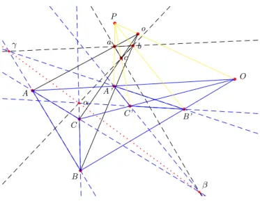
Informal Proof. We have to lift triangle A′B′C′ into a new triangle abc which
is not coplanar with triangle ABC in order to have a configuration of points in which Desargues 3D theorem can be applied. The construction is shown in Figure 10. Here are the main steps: we first construct a point P which lies outside the plane formed by A, B, C, A′, B′, C′ and O. We know such a point
P exists thanks to lemma 8. We then build a line incident to P and O (the point from which triangles ABC and A′B′C′ are perspective) and consider
a third point o on this line (axiom Rk-Three-Points ensures such a point exists and is different from both O and P ). We construct a new point a as the intersection of lines P A′ and oA. We know these two lines intersect
because of Pasch’s axiom and the fact that lines AA′ and P o intersect in
O. We do the same to construct points b and c. Applying Desargues 3D theorem to ABC and abc requires to make sure we have a non-degenerate 3D figure and that abc is a non-degenerate triangle. We also have to make
b A b B b C b O b C’ b A’ b B’ b P bo bc b a b b b b b β γ α
Figure 10: Desargues theorem (3D extrusion) A,B,C,A′,B′,C′,O,α,β and γ are co-planar.
If P is the sun, triangle abc then casts its shadow in A′B′C′.
sure α defined as the intersection of lines BC and B′C′ is the same as the
α of Desargues 3D theorem which is the intersection of BC and bc. This requirement can be satisfied by simply proving that α is incident to bc. The same requirement applies for β and γ. Overall, we have to prove the following statements which are requirements to apply Desargues 3D version (proofs are given below). Note that when applying the theorem, the point o plays the role of point O.
rk{A, B, C} = rk{a, b, c} = 3 rk{A, B, C, a, b, c} ≥ 4
rk{a, b, γ} = rk{a, c, β} = rk{b, c, α} = 2 rk{A, B, γ} = rk{A, C, β} = rk{B, C, α} = 2
Statements rk{A, B, γ} = rk{A, C, β} = rk{B, C, α} = 2 and rk{A, B, C} = 3 are assumptions of the Desargues 2D theorem, therefore their proofs are immediate.
Preliminary Lemmas. We remind the reader that the points A, B, C, A′, B′, C′
and O lie in the same plane. P is a point outside this plane. o is a third point on the line OP . The point a is defined as the intersection of lines P A′ and
oA. Points b and c are defined in a similar way. In this setting, the following lemmas hold:
Lemma 14. rk{A′,B′,O} = rk{A′,C′,O} = rk{B′,C′,O} = 3
Lemma 15. rk{A′, B′, O, P } = rk{A′, B′, O, o} = 4
Lemma 16. rk{A, B, O, a} ≥ 4 rk{A, A′, C, a} ≥ 4
Lemma 17. rk{A, B, O, b} ≥ 4 rk{A, B, O, c} ≥ 4
Lemma 18. rk{o, a} = rk{o, b} = rk{o, c} = 2
Lemma 19. rk{a, c, A, C, β} = rk{a, c, A′, C′, β} = 3
Proof.
rk{A, C, a, c} + rk{A, C, β} ≥ rk{A, C} + rk{A, C, a, c, β} 3 + 2 ≥ 2 + rk{A, C, a, c, β}
Hence rk{A, C, a, c, β} ≤ 3. More as rk{A, C, a, c} = 3, we conclude that rk{A, C, a, c, β} = 3.
General Lemmas. Most proofs are fairly technical, simply using the matroid
axioms of rank. However, some lemmas can be highlighted, especially for their genericity and their pervasive use throughout the proofs. Among them, some stability lemmas state that one of the points of a set characterizing a flat (e.g a plane or the whole space) can be replaced by another one belonging to this flat.
Lemma 20 (Plane representation change). rk{A, B, C} = 3 rk{A, B, C, M} = 3 rk{B, C, M} = 3 rk{A, B, C, P } = 4 ⇒ rk{M, B, C, P } = 4
This lemma is heavily used to prove all possible statements expressing that P lies outside the plane formed by A, B, C, A′, B′, C′, O.
Other lemmas about coplanarity and also upper bound on ranks when merging a plane and a line are convenient as well. They could form the basis of an automation procedure when doing computer-checked formal proofs.
Proving Desargues 3D assumptions.
Lemma 21. rk{A, B, C, a, b, c} ≥ 4
Proof. By lemma 17, we have rk{A, B, O, b} >= 4, hence rk{A, B, C, O, b} ≥ 4. Using axiom R3-alt, we have:
rk{A, B, C, b} + rk{A, B, C, O} ≥ rk{A, B, C, O, b} + rk{A, B, C}
rk{A, B, C, b} + 3 ≥ 4 + 3
Consequently we have rk{A, B, C, b} ≥ 4 and applying axiom R2 twice, it leads to rk{A, B, C, a, b, c} ≥ 4.
Lemma 22. rk{a, b, c} = 3
Proof. By axiom R1 we have rk{a, b, c} ≤ 3.
Let’s prove rk{a, b, c} ≥ 3. By axiom R3-alt, we have:
rk{a, b, c, o, A, B} + rk{o, C, c} ≥ rk{A, B, C, o, a, b, c} + rk{o, c} rk{a, b, c, o, A, B} + 2 ≥ 4 + 2
Hence rk{a, b, c, o, A, B} ≥ 4. Again, using axiom R3-alt we have: rk{a, b, c, o, A} + rk{o, B, b} ≥ rk{a, b, c, o, A, B} + rk{o, b} rk{a, b, c, o, A} + 2 ≥ 4 + 2 Hence rk{a, b, c, o, A} ≥ 4. Applying axiom R3-alt one last time yields:
rk{a, b, c} + rk{o, A, a} ≥ rk{a, b, c, o, A} + rk{a}
rk{a, b, c} + 2 ≥ 4 + 1
Hence rk{a, b, c} ≥ 3. Note that this proof relies on the facts that rk{o, b} = 2 and rk{o, c} = 2 which are proved as lemma 18.
Lemma 23. rk{a, b, γ} = rk{a, c, β} = rk{b, c, α} = 2
Proof. Using axiom R3-alt, we have:
rk{a, c, A, C, β} + rk{a, c, A′, C′, β} ≥ rk{a, c, A, C, A′, C′, β} + rk{a, c, β}
We have rk{a, c, A, C, A′, C′, β} ≥ 4 using axiom R2 and lemma 16. Using
lemma 19, we obtain rk{a, c, β} ≤ 2. As rk{a, c} = 2 (because rk{a, b, c} = 3), we conclude rk{a, c, β} = 2. Proofs for α and γ are the same.
5.3. Formalization in Coq
Formalizing Desargues theorem in Coq is straightforward once we have the axiom system dealing with ranks and proof techniques to handle them nicely. All the above-mentionned lemmas are easily proved and then Desar-gues theorem can be stated as follows:
forall A’ B’ C’ A B C O : Point,
rk(triple A B C)=3 -> rk(triple A’ B’ C’)=3 -> rk(triple A B O)=3 -> rk(triple A C O )=3 -> rk(triple B C O)=3 ->
rk(triple A A’ O)=2->rk(triple B B’ O)=2->rk(triple C C’ O)=2-> rk(couple A A’)=2 -> rk(couple B B’)=2 -> rk(couple C C’)=2 -> rk(triple A B gamma)=2 -> rk(triple A’ B’ gamma)=2 ->
rk(triple A C beta)=2 ->
rk(triple A’ C’ beta) =2 -> rk(triple B C alpha) =2 -> rk(triple B’ C’ alpha) =2 ->
rk(triple alpha beta gamma) <= 2.
This proof in Coq proceeds exactly the same way as the proof presented in the previous section. It is simply a bit more technical and requires a lot of computation to decide equality between sets which are equal but not syntactically equal.
6. Conclusions
We described axiom systems for both projective plane geometry and pro-jective space geometry in Coq. We then formally proved that Desargues property can not be proved in the projective plane but it holds in Fano’s plane and pappusian planes. Finally we proved Desargues theorem in the ≥3-dimensional projective space.
Proofs in the plane were performed in a traditional setting using points and lines. In the projective space, we proposed a new way to express nicely incidence relations thanks to ranks. We designed an axiom system to capture projective geometry using ranks. We also presented some proof engineering techniques that allow having proofs of reasonable size.
Overall, the proofs consist in more than 10000 lines with about 280 lem-mas and their formal proofs4
organized as shown in the figures below.
4
2D 3D Total lines of Coq specs 1800 1800 3600 lines of Coq proofs 4600 5800 10400
Future work includes further formalization of hexamys in Coq. We expect to formalize all the properties enumerated and proved by Pouzergues in [25]. Regarding ≥3-dimensional space, we plan to study how ranks can be used to automatically derive incidence properties. We believe that the genericity of the notation will help the automation process. Geometric algebra can also be an alternative mean to handle projective geometry nicely [10].
References
[1] Y. Bertot and P. Cast´eran. Interactive Theorem Proving and Pro-gram Development, Coq’Art: The Calculus of Inductive Constructions.
Springer, 2004.
[2] M. Bezem and D. Hendriks. On the Mechanization of the Proof of Hessenberg’s Theorem in Coherent Logic. J. of Automated Reasoning, 40(1):61–85, 2008.
[3] J. Brandt and K. Schneider. Using three-valued logic to specify and verify algorithms of computational geometry. In ICFEM, volume 3785 of LNCS, pages 405–420. Springer-Verlag, 2005.
[4] F. Buekenhout, editor. Handbook of Incidence Geometry. North Holland, 1995.
[5] C. Cerroni. Non-Desarguian Geometries and the foundations of Ge-ometry from David Hilbert to Ruth Moufang. Historia Mathematica, 31(3):320–336, 2004.
[6] S.-C. Chou, X.-S. Gao, and J.-Z. Zhang. Machine Proofs in Geometry. World Scientific, 1994.
[7] Coq development team. The Coq Proof Assistant Reference Manual,
Version 8.3. TypiCal Project, 2010.
[9] C. Dehlinger, J.-F. Dufourd, and P. Schreck. Higher-Order Intuition-istic Formalization and Proofs in Hilbert’s Elementary Geometry. In
ADG’00, volume 2061 of LNAI, pages 306–324. Springer-Verlag, 2000.
[10] L. Dorst, D. Fontijne, and S. Mann. Geometric Algebra for Computer
Science. Elsevier, 2007.
[11] J.-C. Filliˆatre and P. Letouzey. Functors for Proofs and Programs. In ESOP’2004, volume 2986 of LNCS, pages 370–384. Springer-Verlag, 2004.
[12] B. Gr´egoire, L. Pottier, and L. Th´ery. Proof Certificates for Algebra and their Application to Automatic Geometry Theorem Proving. Submitted for publication in LNAI as the post-proceedings of ADG’08, 2009. [13] F. Guilhot. Formalisation en Coq et visualisation d’un cours de
g´eom´etrie pour le lyc´ee. TSI, 24:1113–1138, 2005. In french.
[14] C. M. Hoffmann and R. Joan-Arinyo. Handbook of Computer Aided
Ge-ometric Design, chapter Parametric Modeling, pages 519–541. Elsevier,
2002.
[15] P. Janiˇci´c, J. Narboux, and P. Quaresma. The area method : a recapit-ulation. submitted, october 2009.
[16] C. Jermann, G. Trombettoni, B. Neveu, and P. Mathis. Decomposition of geometric constraint systems: a survey. International J. of
Compu-tational Geometry and Application, 16(5-6):379–414, 2006.
[17] E. Kusak. Desargues theorem in projective 3-space. J. of Formalized
Mathematics, 2, 1990.
[18] N. Magaud, J. Narboux, and P. Schreck. Formalizing Projective Plane Geometry in Coq. Submitted for publication in LNAI as the post-proceedings of ADG’08, September 2008.
[19] L. Meikle and J. Fleuriot. Formalizing Hilbert’s Grundlagen in Is-abelle/Isar. In TPHOLs’03, volume 2758 of LNCS, pages 319–334, 2003. [20] D. Michelucci, S. Foufou, L. Lamarque, and P. Schreck. Geometric constraints solving: some tracks. In SPM ’06, pages 185–196. ACM Press, 2006.
[21] D. Michelucci and P. Schreck. Incidence Constraints: a Combinatorial Approach. International J. of Computational Geometry and Application, 16(5-6):443–460, 2006.
[22] F. R. Moulton. A Simple Non-Desarguesian Plane Geometry.
Transac-tions of the American Mathematical Society, (3):192–195, 1902.
[23] J. Narboux. A decision procedure for geometry in Coq. In TPHOLs’04, volume 3223 of LNCS, pages 225–240. Springer-Verlag, 2004.
[24] J. Narboux. Mechanical theorem proving in Tarski’s geometry. In
ADG’06, volume 4869 of LNAI, pages 139–156. Springer-Verlag, 2007.
[25] R. Pouzergues. Les hexamys. Technical report, IREM Nice, 1993. http://hexamys.free.fr.