HAL Id: tel-01702842
https://tel.archives-ouvertes.fr/tel-01702842
Submitted on 7 Feb 2018
HAL is a multi-disciplinary open access archive for the deposit and dissemination of sci-entific research documents, whether they are pub-lished or not. The documents may come from teaching and research institutions in France or abroad, or from public or private research centers.
L’archive ouverte pluridisciplinaire HAL, est destinée au dépôt et à la diffusion de documents scientifiques de niveau recherche, publiés ou non, émanant des établissements d’enseignement et de recherche français ou étrangers, des laboratoires publics ou privés.
Lise Giorgis-Allemand
To cite this version:
Lise Giorgis-Allemand. Atmospheric pollution and Human reproduction.. Neurons and Cognition [q-bio.NC]. Université Grenoble Alpes, 2017. English. �NNT : 2017GREAS003�. �tel-01702842�
THÈSE
Pour obtenir le grade de
DOCTEUR DE LA COMMUNAUTE UNIVERSITE
GRENOBLE ALPES
Spécialité : Modèles, méthodes et algorithmes en biologie
Arrêté ministériel : 7 août 2006
Présentée par
Lise GIORGIS-ALLEMAND
Thèse dirigée par Rémy SLAMAPréparée au sein de l’Institut pour l’Avancée des Biosciences, centre de recherche Université Grenoble Alpes, INSERM U1209 et CNRS UMR 5309
dans l'École Doctorale Ingénierie pour la Santé, la Cognition et l’Environnement
Pollution atmosphérique et
reproduction humaine.
Atmospheric pollution and human
reproduction.
Thèse soutenue publiquement le 3 février 2017, devant le jury composé de :
M. Denis ZMIROU-NAVIER
PU-PH, Inserm, Rennes, Président et rapporteur M. René ECOCHARD
PU-PH, Hospices Civils de Lyon, Lyon, Rapporteur M. René EIJKEMANS
Professor, Julius center, University Medical Center Utrecht, Membre du jury Mme Pascale HOFFMANN
i
Remerciements
Je remercie mon directeur de thèse, Rémy Slama, de m’avoir confié ce sujet de thèse et pour la confiance qu’il m’a accordée pendant 6 ans et quelques.
Je remercie Denis Zmirou-Navier, René Ecochard, René Eijkemans et Pascale Hoffmann d’avoir accepté d’évaluer ce travail.
Cette thèse s’appuie sur les données de plusieurs cohortes, et je souhaite remercier l’ensemble des personnes impliquées, en particuliers les data-managers, les personnes qui ont recueilli les données, et surtout les participant(e)s.
Je remercie l’ensemble des membres de l’équipe, qu’ils travaillent à l’IAB ou à l’HCE, ou qu’ils soient déjà partis vers d’autres aventures. Merci à mes co-bureaux (Claire, Claire, Karine, Emilie, Emilie, Céline – et encore plus anciennement Coraline et Hadrien) pour les discussions scientifiques et non scientifiques et à Meriem pour les raisons précédentes et pour m’avoir évité de faire des extractions sur les fichiers ncdf.
Merci aussi à ceux en France et à l’étranger avec qui j’ai échangé, en particulier Marie, Sandy, Manuela et José.
ii
Summary
1
Remerciements ... i Summary ... ii List of Tables ... iv List of Figures ... v List of abbreviations ... vi Chapter I: Introduction ... 2 I. French summary ... 4 II. Overview ... 5III. Atmospheric pollution ... 7
1. Sources of atmospheric pollutants ... 7
2. Regulation of atmospheric pollution ... 8
3. Temporal trends ... 9
4. Assessment of exposure to atmospheric pollutants in epidemiological studies ... 10
a. Nearest monitoring station network ... 10
b. Land Use Regression, dispersion and chemical transport models ... 11
c. Personal monitors ... 12
d. Estimating exposures during the right time period ... 14
IV. Human Reproduction ... 15
1. Overview ... 15
2. Definitions of the main fecundity and pregnancy related outcomes ... 15
a. Before fertilization ... 15
b. Between fertilization and pregnancy detection ... 17
c. After fertilization ... 19
3. Human reproduction and atmospheric pollution ... 22
a. Air pollution effect on gametogenesis ... 22
b. Air pollution effect on fecundity, fertility, and fecundability ... 22
c. Air pollution effect on birth weight, preterm delivery and stillbirth ... 25
4. Human reproduction and meteorological parameters ... 26
V. Objectives of the thesis ... 29
Chapter II: Methods ... 32
I. French Summary ... 34
II. OBSEFF study... 35
1. Population ... 35
2. Outcomes definition and statistical analysis ... 36
a. Menstrual cycle characteristics ... 36
b. Time to pregnancy studies... 37
3. Atmospheric pollution ... 40
a. Exposure model ... 40
b. Back-extrapolation and seasonalization. ... 40
c. Exposure windows considered ... 42
4. Authors contributions ... 42
III. ESCAPE study ... 43
1. Population ... 43
2. Atmospheric pollution ... 44
a. Exposure model ... 44
b. Backextrapolation and seasonalization ... 44
c. Exposure windows considered ... 45
d. Residential mobility during pregnancy ... 45
3. Meteorological parameters ... 46
4. Preterm birth definition and statistical analysis ... 47
5. Authors contribution ... 47
Chapter III: Before fertilization: Atmospheric pollution and menstrual cycle ... 50
I. French summary ... 52
II. Research letter, to be submitted to Epidemiology ... 54
III. eAppendix ... 59
1 Conformément aux consignes de l'école doctorale Edisce concernant les thèses rédigées en anglais, chaque chapitre
iii I. French summary ... 72 II. Article ... 73 1. Abstract ... 76 2. Introduction ... 77 3. Methods ... 79 4. Results ... 83 5. Discussion ... 86 6. Conclusion ... 90 7. References ... 91
8. Tables and figures... 94
III. Supplemental material... 102
Chapter V: After fertilization: Effects of Atmospheric pollution on preterm delivery ... 106
I. French summary ... 108 II. Article ... 110 1. Abstract ... 114 2. Introduction ... 115 3. Methods ... 116 4. Results ... 119 5. Discussion ... 121 6. Conclusions ... 124 7. Acknowkedgments ... 125 8. References ... 126
9. Tables and figures... 130
III. Supplement material ... 135
Chapter VI: Discussion ... 150
I. French summary ... 152
II. Main findings... 153
III. Methodological issues ... 153
1. Confounding ... 153 2. Outcomes assessment ... 154 a. Menstrual cycle ... 154 b. Fecundity ... 154 c. Preterm birth ... 155 3. Exposure assessment ... 156
a. Back-extrapolation and seasonalization ... 156
b. Geocoding ... 158
c. Residential mobility ... 158
d. Time space activity ... 159
4. Study design and statistical methods ... 160
a. Menstrual cycle study ... 160
b. Fecundity studies ... 161
c. Preterm delivery study ... 165
IV. Plausibility of the findings ... 169
1. Do air pollutants levels influence menstrual cycle length? ... 169
2. Do air pollutants levels influence fecundity? ... 170
3. Are the reported effects of air pollution on preterm delivery a statistical artefact? ... 171
V. Conclusion ... 173
References ... 176
Annexes ... 194
I. Publications and communications ... 196
II. Comment from Ha and Mendola (American Journal of Epidemiology) ... 199
iv
List of Tables
2
Table I-1: Air quality standards as defined in the EU Ambient Air Quality Directive and WHO Air Quality Guideline (AQG), adapted from (EU, 2015) ... 8
Table I-2: Comparison of various outdoor atmospheric pollution exposures assessment used in epidemiological studies ... 13
Table I-3: Publications on air pollution and fecundity-related outcomes in Human. ... 24
Table I-4: Characteristics of the studies on preterm delivery and PM2.5 exposure reviewed by
Sun et al. (2015) ... 27 Table III-1: Adjusted change in the duration of cycle, follicular and luteal phase associated with atmospheric pollution levels (n=181) ... 58
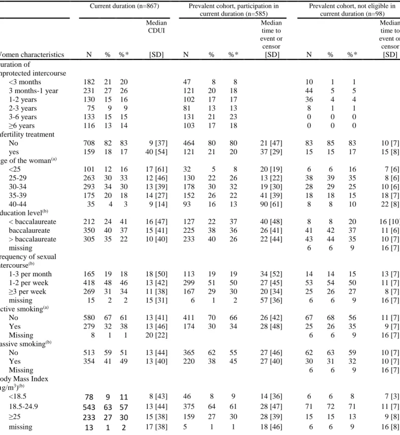
Table IV-1: Characteristics of the population included in current duration or prevalent cohort studies with defined CDUI or time to pregnancy. Note that 585 subjects of the prevalent cohort analysis are also included in the current duration analysis. ... 94
Table IV-2 Association between adjustment factors and time to pregnancy. Current duration and prevalent cohort approach. ... 96
Table IV-3: Atmospheric pollutants and time to pregnancy. Current duration and prevalent cohort approach. ... 97
Table IV-4: Atmospheric pollutants and time to pregnancy. Current duration and prevalent cohort approach, sensitivity analyses ... 98
Table V-1: Characteristics of the Study Population (N=71,493 Live Births from 13 European Cohorts part of ESCAPE project, 1994-2010). ... 130
Table V-2: Associations Between Atmospheric Pollutants and Preterm Birth (Pooled Analysis of 13 European Cohorts part of ESCAPE project, 1994-2010). ... 132
Table VI-1: Summary of the features of the study designs for human fecundity ... 163 Table VI-2: Possible bias in the study designs used to study fecundity and possible solutions. ... 164
v
List of Figures
3
Figure I-1: Evolution of emission of pollutants in mainland France with their sources between
2000 and 2014 (Commissariat général au développement durable, 2015) ... 7
Figure I-2: Percentage of the EU urban population potentially exposed to air pollution exceeding EU air quality standards, (EU, 2011) ... 9
Figure I-3: Evolution of SO2, NO2 and PM10 concentrations over 2000-2014 in France (Commissariat général au développement durable, 2015) ... 9
Figure I-4: Location of background stations measuring NO2 and PM10 in France between 2002 and 2009 ... 11
Figure I-5: Example of the use of GPS data with SIRANE dispersion model with a 10x10 m resolution for PM10 in Grenoble, France ... 12
Figure I-6: Phases of the menstrual cycle ... 16
Figure I-7: gestational age, preterm delivery and pregnancy losses ... 21
Figure I-8: overview of the timeline of reproduction-related outcomes (adapted from Slama, 2014) ... 29
Figure II-1: urinary level of a progesterone metabolite (pregnanediol-3-alpha-glucuronide, PdG) for one study participant ... 36
Figure II-2: Exposures windows and study design, OBSEFF study ... 39
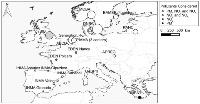
Figure II-3: Map of cohorts included in the ESCAPE preterm delivery study ... 43
Figure IV-1: Study design, example for five women (A to E) ... 99
Figure IV-2: Flow chart ... 100
Figure IV-3: Locations of home addresses of the 544 women included in the current duration analysis with levels of NO2 estimated in year 2009 with the air pollution model. ... 101
Figure V-1: Localization of the study areas within Europe and pollutants assessed at each location. The surface of the circle is proportional to the number of subjects in each center. 13 European Cohorts part of ESCAPE project, 1994-2010. ... 133
Figure V-2: Preterm birth and A) Temperature (first trimester), B) Humidity (whole pregnancy; discrete time survival model) and C) Atmospheric pressure first trimester average.. 134
Figure VI-1: Exposure to PM2.5 during whole pregnancy and preterm delivery in studies using a survival model or a matched case-control. ... 171
vi
List of abbreviations
CDUI: Current Duration of Unprotected Intercourse (outcome of the current duration approach) CI: confidence interval
ESCAPE: European Study of Cohorts for Air Pollution Effects EU: European Union
GIS: Geographic Information System GPS: Global Positioning System hCG: Human Chorionic Gonadotropin HR: Hazard Ratio
ICSI: IntraCytoplasmic Sperm Injection
IGN: Institut National de l'information Géographique et forestière IVF: In Vitro Fertilisation
INERIS: Institut National de l’EnviRonnement Industriel et des RisqueS IQR: Interquartile Range
LH: luteinizing hormone LMP: last menstrual period LUR: Land Use Regression
NO2: nitrogen dioxide
NOX; nitrogen oxides
OBSEFF: OBSErvatoire de la Fertilité en France OR: Odds Ratio
O3: ozone
PM: particulate matter
PM10: particulate matter with aerodynamical diameter of less than 10 µm
PM2.5: particulate matter with aerodynamical diameter of less than 2.5 µm
PMcoarse or PM10-2.5: particulate matter with aerodynamical diameter between 2.5 µm and 10 µm
SO2: sulfur dioxide
TR: Time Ratio
TTP: Time To Pregnancy
2
I.
Chapter I
4
I. French summary
L’impact de certaines expositions environnementales -en particulier la pollution atmosphérique- sur la santé humaine est bien documenté et établi. La pollution atmosphérique peut venir de sources naturelles (volcans) ou anthropiques (trafic routier, industries, chauffage domestique) et est composée d’une multitude de gaz et de particules. Une fraction importante de la population est exposée à la pollution atmosphérique ; ses effets sur la mortalité et la santé cardiovasculaire et respiratoire sont connus, et un effet de l'exposition durant la grossesse sur le poids de naissance ou la croissance fœtale est probable. En revanche, la capacité des couples à concevoir et les paramètres de la fertilité féminine ont été très peu étudiés. Pourtant, la question d’une association entre pollution atmosphérique et fertilité des couples mériterait d’être approfondie en raison des résultats des quelques études animales et humaines existantes. La reproduction est une succession d’étapes qui commencent in utero avec la formation de l’appareil reproducteur. Un effet délétère sur la reproduction pourrait se produire à différentes étapes, que ce soit antérieures (formation des gamètes) ou au cours de la grossesse (implantation de l’embryon, fonction cardio-vasculaire maternelle).
L’objectif de ce doctorat est de mieux documenter un effet éventuel de la pollution atmosphérique sur la fonction de reproduction humaine et tout particulièrement :
1) Avant la conception : étudier l’association entre la pollution atmosphérique et les caractéristiques du cycle menstruel,
2) Autour de la conception : étudier l’association entre la pollution atmosphérique et la probabilité de grossesse en France en utilisant deux designs d’études sur la même population
3) Le déroulement de la grossesse : étudier l’association entre la pollution atmosphérique et les naissances prématurées.
5
II. Overview
In the last centuries, human populations have caused and faced numerous environmental, technological and societal modifications. Many of them are positive and save lives -the development of hygiene, the invention of antibiotics, wider access to clean water, electricity, health care, contraception and education. The implementation of these changes is not uniform within and between populations. In 1990, 76 % of the World population used improved drinking water source and this proportion increased to 91 % in 2015 (WHO and UNICEF, 2015). Life expectancy at birth increased by in average 6 years for children born in 2012 compared to those born in 1990 and this improvement has been seen across all country-income groups (WHO, 2014). Focusing on maternal and child health, globally, maternal mortality felt by 44 % between 1990 and 2015, but the number of maternal deaths was still estimated to be 303,000 in 2015 (WHO et al., 2015). Even if huge progresses have been done in the past decades, there still are margins of improvements and a large geographical heterogeneity. For example, 99 % of the maternal deaths occurring in 2015 happened in developing countries which include 90 % of the number of births worldwide. 66 % of the total number of maternal deaths occurred in Sub-Saharan Africa (26% of the number of birth worldwide) and 22% in Southern Asia (8% of the
number of birth worldwide) (WHO et al., 2015)4.
Amongst all the pollutants generated by human activities, atmospheric pollution is one of the most studied. The London Smog of 1952, causing more than 3,000 deaths (Bell and Davis, 2001), has been a turning point in the study of the effects of atmospheric pollution on health. The most industrialized countries have taken measures to fight air pollution, but the problem in rapidly emerging and newly industrialized countries such as India and to some extent China
remains. In 2012, an average level of PM10 (particulate matter with aerodynamical diameter of
less than 10 µm) of 229 µg/m3 was measured in Delhi, India, while in 2013, an average level
of PM10 of 108 µg/m3 was measured in Beijing, China, and of 141 µg/m3 in Dakar, Senegal.
These levels are far higher than the levels observed in Paris, France (average level of PM10
measured in 2014 of 28 µg/m3) or in Ottawa, Canada (average level measured in 2013 of 11
µg/m3).5 Thus, there still are margins of improvements and a large geographical heterogeneity
for levels of atmospheric pollution too.
4 Number of births worldwide estimated from “The State of the World’s Children 2016 Statistical Tables”,
UNICEF, June 2016.
6 Atmospheric pollution can have various effects on human health at the short and long
terms. WHO classified air pollution as carcinogenic for humans6 and estimated that in 2012,
90% of the world population was exposed to levels of particulate matter higher than the WHO Air Quality Guidelines, and that about 3 million deaths were due to particulate air pollution (WHO, 2016). Mortality, hospital admission and impaired lung function (symptoms of bronchitis) increase with atmospheric pollution (Brunekreef and Holgate, 2002). Air pollution also affects cardiovascular system (Dockery, 2001; Du et al., 2016) and have acute effect on respiratory system (Goldizen et al., 2016). As we will see later, air pollution may also affect reproductive health.
7
III. Atmospheric pollution
1. Sources of atmospheric pollutants
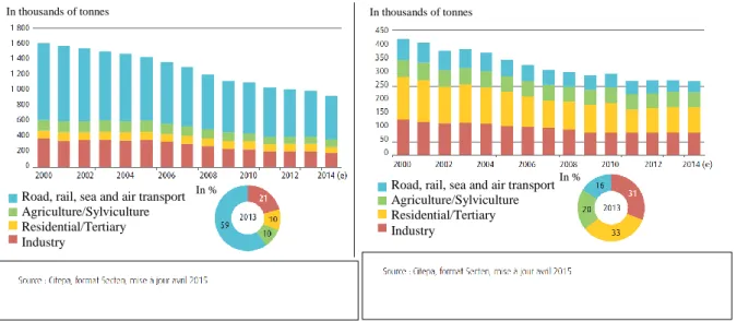
Air pollution is a complex mixture of gases and particulate matter emitted from various
natural and anthropogenic sources (Figure I-1). Nitrogen oxides (NOX, nitrogen oxides, which
include nitrogen dioxide, NO2) are mostly created by anthropogenic emission and particularly
combustion of fossil fuels from stationary sources (industries, power plant, house heating) or mobile sources (cars and other vehicles). In an urban context, nitrogen oxides are often considered as a marker of traffic-related air pollution (Cyrys et al., 2012; Favarato et al., 2014; Hamra et al., 2015). Particulate matter (PM) composition include many organic and inorganic materials from natural sources, such as volcanos or seas, but also man-made sources, such as factories, motor vehicles emissions, construction activities…). The exposure in urban areas is mostly due to anthropogenic sources such as heating, traffic and industry. (EU, 2015; Yang and Omaye, 2009). In addition to chemical composition, particulate matter can be characterized by
their aerodynamical diameter: up to 10 µm (PM10) or below (up to 2.5 µm: PM2.5, up to 1 µm:
PM1, or between 2.5 and 10 µm: coarse fraction, PM10-2.5).
Figure I-1: Evolution of emission of pollutants in mainland France with their sources between 2000 and 2014 (Commissariat général au développement durable, 2015)
A) NOX B) PM10
Road, rail, sea and air transport Agriculture/Sylviculture Residential/Tertiary Industry
Road, rail, sea and air transport Agriculture/Sylviculture Residential/Tertiary Industry
In thousands of tonnes In thousands of tonnes
In %
8 Meteorology is an important determinant of atmospheric pollution as it influences both emissions (more heating in cold days), dispersion -i.e. the transport of pollutants from their source- of pollutants (through wind and other weather conditions) and atmospheric chemical
reactions (through sunlight for ozone). Anthropogenic emissions of NO2 and PM are usually
higher in the period of the year with the lowest temperatures due to heating sources (heating oil, wood). Wind influences long range transport of stable pollutants as for example black
carbon -part of PM2.5 obtained from an incomplete combustion- that can be observed as far as
in Artic (Law and Stohl, 2007). Wind, temperature and solar radiation influence the ground and the atmospheric boundary layer (the part of the atmosphere that is influenced by the planetary surface, with a thickness about 1 km), generating turbulence mixing. When the atmospheric boundary layer is stable, an inversion layer can appear, corresponding to higher temperature at higher height. Then, the atmospheric convection that occurs in neutral and unstable atmospheric boundary layer stops, impacting dispersion and dilution of atmospheric pollution and leading to the formation of fogs (Cushman-Roisin, 2014; Sportisse, 2008).
2. Regulation of atmospheric pollution
Atmospheric pollution is regulated and measured in many places of the world. The World Health organization (WHO) has issued guidelines and in the European Union (EU), additional guidelines values are defined by the Ambient Air Quality Directive. Guidelines values exist in particular for particulate matter and nitrogen oxides (Table I-1), which will be the major pollutants developed in this manuscript. In France, air quality monitoring stations measure these
pollutants on an hourly basis in urban areas with more than 100,000 inhabitants7.
Table I-1: Air quality standards as defined in the EU Ambient Air Quality Directive and WHO Air Quality Guideline (AQG), adapted from (EU, 2015)
EU Air Quality Directive WHO AQG
Pollutant Averaging period Objective and legal
nature Concentration Comments Guideline PM10 1 day Limit value 50 µg/m3
Not to be exceeded on more
than 35 days per year 50 µg/m
3 (a)
PM10 Calendar year Limit value 40 µg/m3 20 µg/m3
PM2.5 1 day 25 µg/m3 (a)
PM2.5 Calendar year Limit value 25 µg/m3 10 µg/m3
NO2, NOX 1 hour
Human health limit
value 200 μg/m
3 not to be exceeded on more
than 18h per year 200 µg/m
3
NO2, NOX Calendar year Human health limit
value 40 μg/m
3 40 μg/m3
NO2, NOX 1 hour Alert (b) threshold 400 μg/m3
(a) 99th percentile (3 days/year)
(b) To be measured over 3 consecutive hours at locations representative of air quality over at least 100 km2 or an entire zone or
agglomeration, whichever is the smaller.
Sources: EU, 2008; WHO, 2006a; WHO, 2008; EU 2015
9 3. Temporal trends
Since a few decades and with more and more stringent regulation, the environmental
levels declined in Europe (EU, 2011) (Figure I-2) and in France (Figure I-3) for NO2 and PM10.
This improvement is not observed in all regions of the world; PM2.5 annual concentrations
decreased between 2008 and 2013 in high-income regions (Americas, Europe, Western Pacific) but increased in other regions (WHO, 2016).
Figure I-2: Percentage of the EU urban population potentially exposed to air pollution exceeding EU air quality standards, (EU, 2011)
Figure I-3: Evolution of SO2, NO2 and PM10 concentrations over 2000-2014 in
France (Commissariat général au développement durable, 2015)
(Index=100 corresponds to concentrations in 2000)
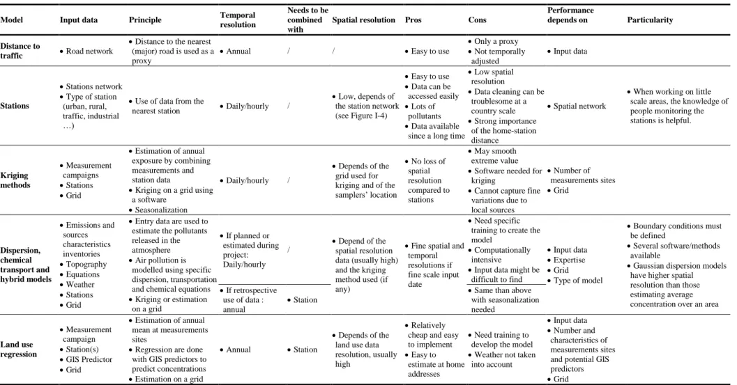
10 4. Assessment of exposure to atmospheric pollutants in epidemiological studies Various methods are used to estimate exposure to atmospheric pollution in environmental epidemiology. Table I-2 (page 13) summarizes these methods while the most frequently used ones will be described below.
a. Nearest monitoring station network
Many countries have a national network of air quality monitoring stations to measure regulated atmospheric pollutants outdoor levels; with stations mostly located in large urban areas or near industrial sites. Using data from monitoring network is often done to estimate exposure to atmospheric pollutants for participants in epidemiological studies as data can be accessed easily (example of studies: Chang et al., 2015; Faiz et al., 2012; Slama et al., 2013). The home address of each subject is generally assigned to the nearest background station functioning during the study period. As most of the monitoring stations are located in cities and as there are only a few ones in each city, the spatial resolution of this approach is quite low (see Figure I-4 for the spatial resolution in France). Monitoring stations data are generally representative of daily temporal variations of atmospheric pollution in a wide area, but only
representative of the exposure levels in a small area around them. Regarding NO2, in a study
conducted with passive samplers in four European cities, more between-site variation was observed than within-site and the spatial contrasts were stable from a measurement campaign to another (Lebret et al., 2000) and in Munich, Germany, the daily averages concentrations were correlated between 0.5 and 0.9 across the seven monitors (Slama et al., 2007). In 36 areas included in European Study of Cohorts for Air Pollution Effects (ESCAPE), there was a large spatial variability observed within study areas, with more variability in traffic than in background sites (Cyrys et al., 2012). Regarding PM, in 20 areas included in ESCAPE,
significant within-area variations was observed for PMcoarse and PM2.5 absorbance compared to
between-areas but not for PM10 and PM2.5; although the within-area variations were smaller for
those two pollutants, a clear spatial contrast within each area still existed between them too
(Eeftens et al., 2012a). Daily concentrations of PM10 between an urban (Vienna) and a rural
station (Streithofen) separated by 30 km (Puxbaum et al., 2004) in Austria had a coefficient of correlation of 0.68 over a year, with higher correlation in summer (0.78) than winter (0.67) (Gomiscek et al., 2004).
11 Figure I-4: Location of background stations measuring NO2 and PM10 in France
between 2002 and 2009
b. Land Use Regression, dispersion and chemical transport models
The need to rely on exposure models with higher spatial resolution than monitoring networks has led to the development of atmospheric pollution fine scale models such as dispersion models and land use regression (LUR) models. Dispersion and chemical transport modellings use emission data and dispersion or chemical equations to estimate fine scales map of atmospheric pollution (Valari et al., 2011). Land use regression relies on land use data (traffic and population densities, greenspaces, industries …), on specific measurements campaigns and on one permanent background air quality monitoring site in order to estimate yearly averages (Beelen et al., 2013; Hoek et al., 2008). Data from air quality monitoring stations can be used to back-extrapolate the yearly average estimated by a LUR model to the subject-specific exposure window of interest (Pedersen et al., 2013a; Slama et al., 2007). Spatial resolution can go from a few meters (see as an example a dispersion model in Figure I-5, next page) for exposure models developed for cities to kilometers for country scale exposure models. In a comparison of the performance of LUR and dispersions models developed for the same area, de Hoogh et al., (2014) observed that the exposure levels at residential home addresses
Legend
stations measuring :
NO2
12 estimated from exposures models developed in 13 Europeans area were better correlated for NO2 than for PM10 and PM2.5.
c. Personal monitors
Personal atmospheric pollutants monitors carried by study subjects allow to take into account all the micro-environments in which subject spends time during the day (indoors, outdoors, during commuting …). The cost and weight of the samplers -for PM in particular- make them difficult to be carried for a long time and to be used at a large scale. So far, in the context of birth cohorts, very few studies relied on personal monitors (e.g. Slama et al., 2009). As done for example in a feasibility study in Grenoble, it is possible to combine monitoring campaigns at home with a dispersion model and the use of GPS data to take into account space time activity, (Ouidir et al., 2015) (Figure I-5).
Figure I-5: Example of the use of GPS data with SIRANE dispersion model with a 10x10 m resolution for PM10 in Grenoble, France
PM10 (µg/m3) 28 29 30 31 34 38 45
13
Table I-2: Comparison of various outdoor atmospheric pollution exposures assessment used in epidemiological studies
Model Input data Principle Temporal
resolution
Needs to be combined with
Spatial resolution Pros Cons
Performance
depends on Particularity
Distance to
traffic Road network
Distance to the nearest (major) road is used as a proxy
Annual / / Easy to use
Only a proxy Not temporally adjusted Input data Stations Stations network Type of station (urban, rural, traffic, industrial …)
Use of data from the
nearest station Daily/hourly /
Low, depends of the station network (see Figure I-4)
Easy to use Data can be accessed easily Lots of pollutants Data available
since a long time
Low spatial resolution
Data cleaning can be troublesome at a country scale Strong importance of the home-station distance Spatial network
When working on little scale areas, the knowledge of people monitoring the stations is helpful. Kriging methods Measurement campaigns Stations Grid Estimation of annual exposure by combining measurements and station data
Kriging on a grid using a software
Seasonalization
Daily/hourly /
Depends of the grid used for kriging and of the samplers’ location No loss of spatial resolution compared to stations May smooth extreme value Software needed for
kriging
Cannot capture fine variations due to local sources Number of measurements sites Grid Dispersion, chemical transport and hybrid models Emissions and sources characteristics inventories Topography Equations Weather Stations Grid
Entry data are used to estimate the pollutants released in the atmosphere Air pollution is
modelled using specific dispersion, transportation and chemical equations Kriging or estimation on a grid If planned or estimated during project: Daily/hourly / Depend of the spatial resolution data (usually high) and the kriging method used (if any)
Fine spatial and temporal resolutions if fine scale input date
Need specific training to create the model
Computationally intensive
Input data might be difficult to find
Input data Expertise Grid Type of model
Boundary conditions must be defined
Several software/methods available
Gaussian dispersion models have higher spatial resolution than those estimating average concentration over an area If retrospective
use of data : annual
Station Same than above with seasonalization needed Land use regression Measurement campaign Station(s) GIS Predictor Grid Estimation of annual mean at measurements sites
Regression are done with GIS predictors to predict concentrations Estimation on a grid
Annual Station
Depends of the land use data resolution, usually high
Relatively cheap and easy to implement Easy to
estimate at home addresses
Need training to develop the model Weather not taken
into account
Input data Number and
characteristics of measurements sites and potential GIS predictors Grid References: Basagaña et al., 2012; de Hoogh et al., 2014; Lepeule et al., 2010; Sellier et al., 2014; Wang et al., 2015
14
d. Estimating exposures during the right time period
Some exposure models with a high spatial resolution may have a low temporal resolution. For example, LUR models estimate yearly average of exposures. In the case of dispersion models, the method implies to estimate hourly measurements of pollutants in the area considered, but as this represents a huge amount of data, sometimes only the yearly averages are stored and the exposures simulated at a higher temporal resolution are discarded. In environmental epidemiology, however, it is often useful to have exposure levels at subject-specific time periods (e.g. during fetal life) and sometimes back in time (e.g. pregnancy cohort study with recruitment in the 1990’s) (Slama et al., 2007). This can be accommodated in two way; the first one is to ask ahead of the project for the daily or hourly data estimated by the dispersion models used for regulatory purposes whenever possible; the second one is to use data from air quality monitoring stations to extrapolate back in time (“back-extrapolate”) and at the appropriate time period (“seasonnalize”). Two different possibilities to seasonnalize and back-extrapolate exposure will be detailed in the method sections, one assuming that spatial exposures in an area varies similarly over time than a reference monitoring station (Methods, III.2.2.b, page 44) (Pedersen et al., 2013a) and the other that the spatial contrasts at the country scale were invariant over time (Methods, II.3.3.b, page 40).
15
IV. Human Reproduction
1. Overview
Human reproduction is a complex chain of events. The related outcomes expand from intrauterine life (congenital anomalies, fetal growth and rates of miscarriages, stillbirths, and preterm births) to puberty (puberty onset), and to the fecund period (gametogenesis, time to pregnancy, embryo’s implantation, menopause onset) until pregnancy (health of the pregnant woman). Studying risk factors of altered fecundity and pregnancy related outcomes is important because the health burden entailed can be large (Slama et al., 2014). This is all the more important in the context of a plausible deterioration of male fecundity parameters in some areas of the world (Auger et al., 1995; Carlsen et al., 1992). Although designs to study pregnancy outcomes such as birthweight are relatively straightforward (cohort of pregnant women, birth registers), studying fecundity is a little more complicated as it implies to identify couples at risk to have a pregnancy and to try including couples remaining infertile.
The outcomes that are considered in this thesis will be described more in details in this chapter.
2. Definitions of the main fecundity and pregnancy related outcomes
a. Before fertilization
i. Oogenesis and the menstrual cycle
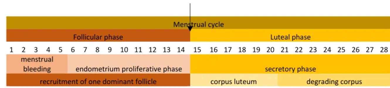
Menstrual cycle is the cyclic phenomenon that prepares the female body for pregnancy. It occurs repeatedly (about 450 times for modern women, Thomas and Ellertson, 2000) between puberty and menopause and is controlled by hormonal changes and feedback mechanisms occurring during ovarian and uterine cycles. The first day of the cycle is by convention the first day of the menstrual bleeding (Figure I-6). The ovarian cycle begins by the follicular phase, during which the recruitment of a dominant follicle occurs through multiple follicular waves. Meanwhile, the estradiol secreted by the growing follicle(s) supports the proliferation of the endometrium to prepare the uterus for a possible pregnancy. Peak of estradiol occurs around day 12 and is followed by a rapid increase in luteinizing hormone (LH, delivered by pituitary gland) that triggers ovulation from the dominant follicle around 12 hours later (the pattern in LH surge have variability, Direito et al., 2013). In the second phase -the luteal phase- the follicle that has produced an ovum evolves in corpus luteum under the influence of LH and begins producing progesterone with a peak around 10 days after ovulation. If no fertilization occurs,
16 the cycle ends once no more progesterone is produced. Once the corpus luteum is in function, the endometrium enters the secretive phase, which is the readiness phase to be implanted by a fertilized egg. When implantation occurs, the implanted embryo will give hormonal signal to the corpus luteum to continue producing progesterone. Otherwise, if no fertilization occurs, once no more progesterone is produced, the upper layer of the endometrium degenerates and is evacuated by the menstrual flow (Jones and Lopez, 2013; Wilcox, 2010).
Figure I-6: Phases of the menstrual cycle ovulation
Menstrual cycle
Follicular phase Luteal phase
days 1 2 3 4 5 6 7 8 9 10 11 12 13 14 15 16 17 18 19 20 21 22 23 24 25 26 27 28 uterine cycle
menstrual
bleeding endometrium proliferative phase secretory phase
ovarian cycle recruitment of one dominant follicle corpus luteum degrading corpus
The duration of each phase varies by women and within women between cycles. The variability of the cycle length is greater in years following menarche and preceding menopause (Treloar et al., 1967). Most of the variability in cycle length is due to the follicular phase (Fehring et al., 2006). In the French OBSEFF study (Observatory of Fecundity in France, see Methods), the median cycle length was 28 days (5th-95th percentiles: 23-40, n=127) with a follicular phase lasting in median 18 days (14-27, n=162) and a luteal phase lasting in median 10 days (6-14, n=117) (Rosetta L et al., submitted). In the USA, a study was conducted among 141 women in good health and with regular cycles. This study included 1,060 menstrual cycles and observed a median cycle length of 29 days (95% confidence interval, CI: 22-36), a median follicular length of 16 days (95% CI: 10-22), a median luteal phase of 13 days (95% CI: 9-16) and a median bleeding duration of 6 days (95% CI: 3-8) (Fehring et al., 2006).
Menstrual cycle characteristics are affected by age (Treloar et al., 1967), but can also be associated with ethnicity, smoking status, physical activity, body mass index, alcohol and caffeine consumption, age at menarche, parity, recent oral contraceptive use and marijuana smoking (Jukic et al., 2007; Kato et al., 1999; Liu et al., 2004). Environmental exposures are suspected to influence cycle characteristics, including pesticides (Farr et al., 2004), organochlorine compounds (Cooper et al., 2005; Windham et al., 2005), chlorination
by-17 products (Windham et al., 2003) and parabens (Nishihama et al., 2016). No study related to atmospheric pollution has to our knowledge been published.
Cycle length can be monitored using diaries filled daily by women, but, as there are no clear external signs for ovulation, knowing follicular and luteal phases length require collecting biological samples and measuring hormonal metabolites (as done for example by Liu et al,. 2004; or Windham et al., 2005) or using fecundity monitoring devices such as done by Fehring et al. (2006). Ovulation can also be detected by measuring basal body temperature (as done by Harvey et al., 2009). Studying menstrual characteristics implies recruiting women not using any contraceptive methods or to follow-up women planning to discontinue contraception.
ii. Spermatogenesis
In males, from puberty onwards, spermatozoa are created continuously in the testis. In humans, spermatogenesis lasts approximately 74 days to obtain spermatozoa from a spermatogonium (Amann, 2008; Heller and Clermont, 1964). The duration of approximately 64 days is sometimes found, but this estimate ignores the 10 days needed by the proliferation of spermatogonia (Amann, 2008).
Factors influencing spermatogenesis and semen parameters include age (Stone et al., 2013), lifestyle factors (Jensen et al., 2004; Taha et al., 2012) but also occupational exposures (De Fleurian et al., 2009).
b. Between fertilization and pregnancy detection
i. Fecundity, fertility, fecundability and time to pregnancy
The following definitions will be used through all the thesis.
Fecundity is the biological aptitude to conceive and bear a child until birth. This biological parameter cannot be assessed directly and can either be defined for a person or a couple (Leridon, 2007).
Fecundability is the monthly probability to conceive for a couple not using any contraceptive method (Gini, 1926; Slama et al., 2013).
Fertility is a demographic parameter measuring the number of children per woman (Leridon, 2007).
18 Time to pregnancy is the time needed by a woman or a couple not using contraception to obtain a pregnancy ending by a live birth (Baird et al., 1986).
Involuntary infertility is usually defined as a period of unprotected intercourse without succeeding in having a child; one can for example consider 12 or 24 months involuntary infertility. (Habbema et al., 2004; Slama et al., 2012)
As identifying women who have already been pregnant can be done without too much difficulties, the classical design to study fecundity is the pregnancy-based design in which women were asked to provide retrospectively their duration of unprotected intercourse before being pregnant (as done for example in the French PELAGIE cohort by Chevrier et al., 2013 or in the Danish National Birth Cohort by Bach et al., 2015). Fecundability can be assessed by estimating the percentage of women conceiving during the first month of unprotected intercourse (as done in a birth cohort by Slama et al., 2013). The major issue with this retrospective design is that couples never achieving pregnancy are not included (Slama et al., 2014). To include these couples, recruitment should take place before the start of the period of unprotected intercourse (as done for example in LIFE study, Buck Louis et al., 2011; or in Germany for couples using natural family planning, Gnoth et al., 2003) or during this period (as in the French OBSEFF study by Slama et al., 2012 or in the Danish Snart gravid study by Mikkelsen et al., 2009).
Statistical methods and potential biases depend on when the couples were recruited: before the period of unprotected intercourse (incident cohort), during (current duration study if couples are not followed-up, prevalent cohort design otherwise) or after (pregnancy-based). Study designs and biases in time to pregnancy studies have been summarized elsewhere (Slama et al., 2006, 2014, Weinberg et al., 1993, 1994) and will be further discussed here in the discussion (Chapter IV, III.4, page 161).
Fecundity and fecundability depend on male and on female factors that can impact sperm or egg quality or viability of the embryo, such as age (Mutsaerts et al., 2012), active smoking (Baird and Wilcox, 1985), body mass index (Gesink Law et al., 2007), lifestyle (Curtis et al., 1997; Hassan and Killick, 2004), medical treatment and health (female asthma for example is associated with prolonged time to pregnancy, Juul Gade et al., 2014).
19
ii. Pregnancy detection
Pregnancy can be detected by the woman noticing a delay in her menstrual periods. It can also be detected earlier by measures in blood or urine of Human Chorionic Gonadotropin (hCG), a hormone secreted after implantation.
c. After fertilization
i. Gestational age at birth, preterm and very preterm delivery
Gestational age at birth is the time between the beginning of the last menstrual period and birth; it corresponds approximately to the time between fertilization and birth, with two weeks being added to account for the duration of the follicular phase and for the time between ovulation and fertilization (Figure I-7, page 21). The gestational age estimated from the last menstrual period can be corrected at the first ultrasound measurement if the size of the embryo is smaller or bigger than expected at this age from reference charts (Gjessing et al., 2007). Although ultrasound measurements give a good estimate of the delivery date, in term of epidemiology, it can be debated to rely on it because if an exposure has an effect on the early embryo development, correcting the gestational age might introduce bias in the association to be identified (Basso and Olsen, 2007; Lynch and Zhang, 2007).
Preterm delivery corresponds to births occurring before 37 completed weeks of gestation while very preterm delivery is usually defined as births occurring before 32 completed weeks of gestation (Figure I-7). As the newborn is still immature after 37 completed weeks of gestation, there is an increased risk of morbidity and mortality for newborns born before term (Goldenberg et al., 2008). Preterm births might be due to malformations (Purisch et al., 2008), maternal pathologies such as infections (Rours et al., 2011) or pre-eclampsia (hypertensive diseases of unknown causes occurring in 2-8% of pregnancies, Ananth et al., 2013; English et al., 2015; Wallis et al., 2008, with risk factors including obesity, age and multiple pregnancy; Duckitt and Harrington, 2005; Sibai et al., 2005). Other factors such as maternal smoking, maternal obesity and maternal obstetric history (parity, previous history of preterm birth) and gender of the fetus are also associated with increased preterm delivery risk (reviewed by Os et al., 2013).
20
ii. Pregnancy losses, miscarriages and stillbirths
Pregnancy losses occurring before the pregnancy detection are called early pregnancy loss, while those occurring once the fetus is viable are called stillbirth (opposed to live birth, which is when the child is born alive, even if he decease shortly after birth) (Wilcox, 2010). The legal limit between miscarriage and stillbirth is different by country8. In France, to be
considered viable, a child must be born with a gestational age of at least 22 weeks with a birthweight of at least 500g.
Pregnancy losses occurring between fertilization and pregnancy detection might be unnoticed. This might concern a large number of pregnancies; in a study conducted between 1982 and 1985, 25% of the pregnancies ended within 6 weeks after LMP (Wilcox et al., 1990). Risk factors for stillbirth include prolonged pregnancy, congenital abnormalities, old maternal age, maternal infections and lifestyle factors (Lawn et al., 2016). For miscarriage, risk factors include chromosomal aberrations, maternal obstetric history, infections, uterine malformations, lifestyle factors, and age (García-Enguídanos et al., 2002).
21 Figure I-7: gestational age, preterm delivery and pregnancy losses
0 6 7 13 14 20 21 27 28 34 35 41 42 48 49 55 56 62 63 69 70 76 77 83 84 90 91 97 98 104 105 111 112 118 119 125 126 132 133 139 140 146 147 153 154 160 161 167 168 174 175 181 182 188 189 195 196 202 203 209 210 216 217 223 224 230 231 237 238 244 245 251 252 258 259 265 266 272 273 279 280 286 287 293 294 300 301 307 308 314
44
42 43
24
18 19 20
25 26
30 31 32 33 34 35
38 39 40 41
17
29
36 37
13 14 15 16
6 7 8 9 10 11
27 28
0 1 2 3 4 5
12
21 22 23
First trimester Second trimester Third trimester
Entire pregnancy
sources : (Slama et al., 2014; Wilcox, 2010)
Early pregnancy losses
Preterm birth Term birth Very preterm birth
Gestationnal age (weeks) Days since last menstrual period Last menstrual period Pregnancy detection Implantation Ovulation Stillbirth Miscarriage Live births Pregnancy losses
22 3. Human reproduction and atmospheric pollution
Several studies were conducted on the relation between human reproduction and atmospheric pollution, with some aspects more studied than others. In this section, the studies describing a possible effect of atmospheric pollution on human reproduction are reviewed.
a. Air pollution effect on gametogenesis
On the female side, to our knowledge, no study has been conducted on the possible influence of atmospheric pollution on menstrual function in Human yet.
Studies on sperm quality have been recently reviewed by Deng et al. (2016), Fathi Najafi et al. (2015) and Lafuente et al. (2016). The first review included the results from 10 studies and performed a meta-analysis concluding that there was a trend for impaired sperm quality in the most exposed group compared to the lowest exposure group (Deng et al., 2016). The second review included 17 studies and concluded, without a meta-analysis, that air pollution influence DNA fragmentation and sperm morphology but not sperm motility (Lafuente et al., 2016). A previous review and meta-analysis focused on slightly different publications than Deng et al. (2016) concluded on the contrary that air pollution was associated with decreased sperm motility but that there was no evidence regarding the other parameters (Fathi Najafi et al., 2015). The fact that the reviews did not share the same conclusion is probably due to the difficulty that reviews had to compare the various existing studies on this topic, in particular due to the lack of standardized measurements of sperm parameters.
b. Air pollution effect on fecundity, fertility, and fecundability
The studies conducted on fecundity related outcomes have been recently reviewed (Checa Vizcaíno et al., 2016; Frutos et al., 2015) and are summarized by outcome in Table I-3, restricting to studies in the general population. In the general population, four studies were conducted: one on fecundability (Slama et al., 2013), two on fertility rates (Koshal et al., 1980; Nieuwenhuijsen et al., 2014) and one on incident involuntary infertility (Mahalingaiah et al., 2016). Few studies were also conducted on specific populations, generally on couples resorting to In Vitro Fertilization (IVF) or Intracytoplasmic Sperm Injection (ICSI) (Legro et al., 2010; Perin et al., 2010a, 2010b). Most of the studies on fecundity related outcomes reported that atmospheric pollution was associated with altered reproductive outcomes. No study was conducted on time to pregnancy in a general population and the three studies focusing on couples with difficulties to conceive were not able to adjust for possible cofounders except age
23 or season. The study on fecundability observed reduced fecundability with increased exposure
to NO2 and PM2.5 around contraception stop (Slama et al., 2013) while the study on incident
infertility observed a small increase in risk of involuntary infertility when distance to traffic was used to assess exposure, but not when it was assessed using a dispersion model (Mahalingaiah et al., 2016). With the design of this last study, it was not possible to consider short-term effects of air pollutants as the exact diagnosis date was unknown and set as the average between the dates of two questionnaires separated by 2 years.
24 Table I-3: Publications on air pollution and fecundity-related outcomes in Human.
Outcome Study Location Period Population Sample size Exposure windows Exposure considered,
(distribution) and exposure model
Adjustment factors Statistical
model
Main findings (95% CI)
Fecundability Slama et al., 2013 Teplice, Czech Republic 1994-1996 Birth cohort: pregnancy-based fecundability design. Planned pregnancies only 1,916 25% obtained pregnancy in the first month of the period of unprotected intercourse
lag1 :30 days after contraception stop lag2: 30 days before
contraception stop [lag1 lag2]: from 30
days before contraception stop to 30 days after (25th, 50th, 75th percentiles in lag1, µg/m3) PM2.5, (27, 34, 43) O3, NO2, (31, 36, 40) SO2
Model= one station for the whole study area, <12 km from home
Maternal smoking, body mass index, maternal age at the start of the period of unprotected intercourse, education, marital status, parity, respiratory epidemic in the previous month, time of the start of the period of unprotected intercourse (spline) Binomial regression model with a logarithmic link
Fecundability ratio per each increase by 10µg/m3in exposure: [lag1] PM2.5: 0.96 (0.86;1.07) O3 1.06 (0.97;1.15) NO2 0.71 (0.57;0.87) SO2 0.99 (0.94;1.05) [lag1 lag2] PM2.5: 0.78 (0.65;0.94) O3 1.04 (0.93;1.17) NO2 0.72 (0.53;0.97) SO2 0.94 (0.85;1.04) Incident involuntary infertility (attempted conception ≥12 months without success). Mahalingaiah et al., 2016 USA 1993-2003 Prospective cohort (Nurses’ Health Study II). Questionnaires every 2 years 36,294 (2,508 cases for 213,416 person-years) 2 years prior diagnosis 4 year prior diagnosis Cumulative: 1998 to current
(Median and IQR during the 2 years average, µg/m3)
PM10 (24, 7)
PM2.5 (15, 4)
PMcoarse (9, 5)
Nationwide spatiotemporal model,
Exposure at home address
Age, race, calendar year, region, current body mass index, smoking, oral contraceptive use, age at menarche, overall diet quality, history of rotating shift work and census tract level median income and home value
Time-varying Cox proportional hazard model
Hazard ratio per 10 µg/m3 increase:
PM10 2 years 1.04 (0.96;1.11) 4 years 0.99 (0.91;1.08) Cumulative 1.06 (0.99;1.13) PM2.5 2 years 0.98 (0.86;1.12) 4 years 0.91 (0.78;1.05) Cumulative 1.05 (0.93;1.20) PMcoarse 2 years 1.10 (0.981.23) 4 years 1.05 (0.93;1.19) Cumulative 1.10 (0.99;1.22) Fertility rates (number of children ever born per 1000 ever married women in a given age group)
Koshal et al., 1980 USA, 74 standard metropolitan statistical areas
1970 annual PM per standard
metropolitan statistical area
Income, percentage of families below the low income level, annual temperature, education of females relative to male, availability of medical facilities and rate of net migration
Multivariate linear regressions
Air pollution reduced fertility rates.
Fertility rates (number of live births per 1000 women ages between 15 and 44 by census tract) Nieuwenhuijsen et al., 2014 Barcelona, Spain 2011-2012 Cross sectional study, registries 27,617 births
year 2009 (IQR, µg/m3 by default)
PM10 (2.9) PM2.5 (2.5) PMcoarse (3.5) PM2.5 absorbance (0.7 unit) NO2 (12.0) NOX (26.0)
LUR (ESCAPE), exposure averaged by census tract area
Socioeconomic status, age, percentage of women born outside Spain.
Besag-York-Mollié models
Infertility risk per IQR increase in air pollution: NO2 0.97 (0.94;1.00) NOX 0.99 (0.96;1.02) PM2.5 0.99 (0.96;1.02) PM10 0. 99 (0.97;1.02) PMcoarse 0.88 (0.83;0.94) PM2.5 0.98 (0.95;1.02)
NO2: nitrogen dioxide; NOX: nitrogen oxides; O3: ozone; PM: particulate matter; SO2: sulfur dioxide;
25
c. Air pollution effect on birth weight, preterm delivery and stillbirth
Many studies and reviews have been conducted on birth weight and preterm delivery. Not exhaustively, association of air pollution with (low) birthweight and preterm birth were reviewed by at least eight reviews (Bonzini et al., 2010; Shah et al., 2011; Srám et al., 2005; Stieb et al., 2012), with some reviews focusing only (Bosetti et al., 2010; Lamichhane et al., 2015) or mostly (Backes et al., 2013) on PM and birth outcomes or PM and preterm birth (Sun et al., 2015). The reviews concluded that despite significant heterogeneity between studies, PM (Lamichhane et al., 2015; Shah et al., 2011; Stieb et al., 2012; Sun et al., 2015) and other pollutants (Shah et al., 2011; Stieb et al., 2012) might increase preterm delivery risk. Srám et al. (2005) concluded that it was possible that air pollution increase preterm delivery risk while Bosetti et al. (2010)did not conclude in favor of such an association. Articles included in the review done by Sun and colleagues (2015), the most recent review on the association between
PM2.5 and preterm birth risk, are summarized in Table I-4, page 27.
Reviews by Backes et al. (2013), Bonzini et al. (2010), Lamichhane et al. (2015), Shah et al. (2011), Srám et al. (2005) and Stieb et al. (2012) were in favor of an association between air pollution and birthweight while Bosetti et al. (2010) did not conclude for an association. A
risk-assessment study based on the risk of term low birth weight due to exposure to PM2.5 reported
by Pedersen et al. (2013a) estimated that 24% of total cases (9-37%) in the French urban area of Grenoble and 28% of cases (11-43%) in the bigger French urban area of Lyon were attributable to exposure to PM2.5 (Morelli et al., 2016).
Risk of stillbirth was recently reviewed by Siddika et al. (2016). A meta-analysis was performed on the 13 epidemiological studies identified and the authors concluded were that their results provided suggestive evidence that air pollution is a risk factor for stillbirth.
26 4. Human reproduction and meteorological parameters
Meteorological parameters influence both atmospheric pollution levels and human health (see McMichael et al., 2006, for a review in the context of climate change). Studies sometimes consider meteorological parameters -especially temperature- as confounding factors when studying association between atmospheric pollutants and human reproductive health (e.g. preterm birth: Chang et al., 2015; stillbirth: Faiz et al., 2012; sperm characteristics: Sokol et al., 2006), but most studies adjusted only for season. Some studies focused on the effect of temperature on birth outcomes (reviewed by Strand et al., 2011), climate and birth outcomes (Beltran et al., 2014; Poursafa et al., 2015) and temperature and preterm delivery (Carolan-Olah and Frankowska, 2014). Regarding fecundity, no strong reasons of considering meteorological factors on time to pregnancy or menstrual cycle were found.
27
Study Population (n, % preterm) Location and period
Exposure (air pollution and meteorology)
Statistical model and exposure windows
Main findings (95% CI) regarding preterm birth risk. For results given by IQR increase, the value in parenthesis after the exposure windows corresponds to IQR Brauer et al., 2008 Registers
(n=70,249, 5%) Vancouver, Canada, 1999-2002
CO, NO, NO2, O3, PM10, PM2.5,
SO2, black carbon
Nearest station, LUR, inverse-distance weighting
Logistic regression WP, M1, M1r, M3r
“For the preterm birth outcome of < 37 weeks, we did not observe any consistent associations with any of the pregnancy average exposure metrics except for PM2.5
(inverse distance weighting: OR= 1.06; 95% CI, 1.01–1.11).”
Chang et al., 2015 Register (Atlanta Birth Cohort) (n=175,891, 10.6%) Atlanta, USA 1999-2005 PM2.5 monitoring stations Temperature Monitoring stations
Distributed exposure discrete-time survival model
WP, T1, T2 , T3, M1 4-week lag (week t-3 to t)
Relative risk per one IQR increase in PM2.5
WP (3.1 µg/m3) 1.03 (1.00, 1.06) T3 (5.4 µg/m3) 1.00 (0.99, 1.01)
T1 (5.2 µg/m3) 1.01 (0.99, 1.04) 1rst 4w (5.9 µg/m3) 1.00 (0.99, 1.02)
T2 (5.1 µg/m3) 1.03 (1.01, 1.05) 4 week lag (6.0 µg/m3) 1.00 (0.99, 1.02)
Fleischer et al., 2014 Cross-sectional survey (n=192,900, 3-11%)
24 countries (Africa, Latin America, Asia)
2004-2008
PM2.5
Satellites combined with chemical transport model and monitoring stations, buffer of 50 km around each health facilities
Generalized estimating equation models (nested structure) with logit link
T1, last month
Odds ratio for an increase by 10 µg/m3 of PM
2.5 in month before birth
Whole survey : 0. 96 (0.90, 1.02) China : 1.11 (1.04, 1.17) India : 0.96 (0.91, 1.03)
Gehring et al., 2011a Cohort (PIAMA) (n=3,863, 4%) Netherlands 1996-1997 NO2, PM2.5, soot LUR Logistic regression WP, T1, last month
Odds ratio per one IQR increase
NO2 (IQR in µg/m3) PM2.5 (IQR in µg/m3) Soot (IQR in 10-5m-1)
WP (11) 1.08 (0.80;1.47) WP (5) 1.22 (0.83; 1.80) WP (1) 1.27 (0.96; 1.67) T1 (14) 0.97 (0.73; 1.27) T1 (8) 0.98 (0.75; 1.29) T1 (2) 0.94 (0.72; 1.23) LM (14) 1.08 (0.86;1.36) LM (5) 1.06 (0.84;1.35) LM (1) 1.12 (0.96;1.32) Gray et al., 2014 Register
(n=457,642, 10%) North Carolina, USA 2002-2006
PM2.5, O3
Station and numerical models
Logistic mixed regression WP
Per one IQR increase:
PM2.5: O3: WP (14 µg/m3) 1.01 (0.99, 1.02) WP (6 ppb) 1.02 (0.99, 1.04) Ha et al., 2014 Register (n=423,719, 9%) Florida, USA 2004-2005 PM2.5, O3
Hierarchical bayesian prediction model
Logistic regression WP, T1, T2, T3
Odds ratio per one IQR increase :
O3 (IQR in ppb) PM2.5 (IQR in µg/m3)
WP (7) 1.03(1.01,1.05) WP (2) 1.05(1.04,1.07) T1 (8) 1.01 (1.0,1.03) T1 (3) 1.03 (1.02, 1.04) T2 (8) 1.02(1.01,1.04) T2 (3) 1.12 (1.11, 1.14) T3 (8) 0.99 (0.98,1.01) T3 (3) 1.03 (1.01, 1.04) Hannam et al., 2014 Cohort (North West England Perinatal
Survey) (n=252,170, 7%) England, UK 2004-2008
NO2, NOX, PM10, PM2.5, CO
Seasonalized (monthly) spatial model (1x1 km)
Nearest station
Logistic regression WP, T0, T1, T2, T3
Odds ratio per one IQR increase, Spatio-temporal model NO2: NOX WP 1.10 0.82–1.48 WP 1.03 0.93–1.14 T1 1.08 0.92–1.27 T1 1.04 0.91–1.19 T2 1.07 0.91–1.25 T2 1.08 0.94–1.24 T3 1.01 0.86–1.19 T3 1.00 0.87–1.15 PM10: PM2.5: WP 0.98 0.85–1.12 WP 0.90 0.74–1.11 T1 1.06 0.92–1.21 T1 1.00 0.90–1.12 T2 0.95 0.83–1.09 T2 0.98 0.92–1.05 T3 0.97 0.84–1.11 T3 0.91 0.82–1.02 Huynh et al., 2006 Case-control (Register)
(n=42,692) California, USA 1998-2000
CO (ppm), PM2.5
Nearest station
Conditional logistic regression (matching)
WP, M1, last 2 week
OR, PM2.5, per 10 µg/m3 increase
WP 1.15 [1.15, 1.16]
First month 1.13 [1.13, 1.13]
Last 2 weeks 1.06 [1.05, 1.06]
28
Hyder et al., 2014 Register (662,921, 6%)
Connecticut and Massachusetts, USA 2000-2006
PM2.5
Monitors, satellite
Logistic regression
Model for trimesters included residuals from regressing exposure estimates from the trimester of interest against other trimesters. WP, T1, T2, T3
Air pollution estimated using monitors, Odds ratio per 2.4 µg/m3increase (one IQR)
WP 1.00 (0.99 to 1.02) T1 1.00 (0.99 to 1.02) T2 1.01 (1.00 to 1.02) T3 1.00 (0.99 to 1.01)
Air pollution estimated using satellites model: no association Jalaludin et al., 2007 Register (Midwives Data Collection)
(n=123,840, 5%) Sydney, Australia 1998-2000
CO, NO2, O3, PM10, PM2.5, SO2
Average of all station or matching by postcode
Relative humidity and temperature (tested with linear coding only)
Logistic regression T1, T3r, M1, M1r
Odds ratio by 1 unit increase:
PM10 (µg/m3) PM2.5 (µg/m3) NO2 (pb)
M1r 0.99 (0.98–1.00) M1r 0.98 (0.96–1.01) M1r 1.00 (0.99–1.01) T3r 0.99 (0.98–1.00) T3r 0.98 (0.95–1.01) T3r 1.01 (0.99–1.02)
M1 0.98 (0.97–0.99) M1 0.98 (0.96–1.00) M1 0.97 (0.96–0.98)
T1 0.99 (0.97–1.00) T1 0.98 (0.95–1.01) T1 0.97 (0.96–0.98)
Kloog et al., 2012 Registry (Massachusetts birth registry) (n=634,244, 10 %?) Massachusetts, USA 2000-2008 PM2.5 satellites
Logistic mixed regression models using pre term/full term birth as the outcome (random intercept for census tract)
WP, T3r, M1r
Odds ratio for each 10 µg/m3 increment
M1r 1.00 (0.96;1.04) T3r 0.99 (0.94;1.03)
WP 1.06 (1.01;1.13)
Lee et al., 2013 Hospital-based cohort (n=34,705, 9%) Pittsburgh, USA 1997-2002
PM10, PM2.5 (µg/m3),
O3 (ppb)
kriging method, zip code
Logistic regression T1
Odds ratio by one IQR increase during first trimester: PM10 (8 µg/m3) 1.04 (0.94–1.14)
PM2.5 (4 µg/m3) 1.10 (1.01–1.20)
O3 (17 ppb) 1.23 (1.01–1.50)
Pereira et al., 2014a Birth registry
29,175 women giving birth to 61,688 neonates (6% in reference population) Connecticut, USA 2000-2006 PM2.5, CO, NO2 Station Temperature station
Conditional logistic regression, pregnancies matched by mother WP, T1, T2, T3
WP and T3 are censored
Odds ratio per one IQR increase for PM2.5 (Results with other pollutants not shown)
WP (2 µg/m3) 1.13 (1.00, 1.28)
T1 (3 µg/m3) 1.10 (1.03, 1.17)
T2 (3 µg/m3) 0.93 (0.87, 0.99)
T3 (4 µg/m3) 1.06 (1.00, 1.11)
Pereira et al., 2014b Case-control, Registry 31,567 births for 14,497 women (7% in reference population) Perth, Australia.
1997-2007
PM2.5, CO, NO2, O3
station
Conditional logistic regression, pregnancies matched by mother (same as design as Pereira et al., 2014a)
WP, T1, T2, T3 WP and T3 are censored
Odds ratio per 1 µg/m3 increase in PM 2.5
WP 0.99 (0.95, 1.04) T1 1.00 (0.96, 1.04) T2 1.00 (0.96, 1.04) T3 0.98 (0.94, 1.02)
Association with other pollutants not reported Ritz et al., 2007 Case-control nested in birth cohort
(n=58,316) California, USA 2003 CO, NO2, O3, PM2.5 Station ZIP codes Logistic regression WP, T1, 6 weeks before birth
“exposure to the traffic-related pollutants -CO and fine particles- mostly during the first trimester but also possibly high exposures prior to delivery are associated with preterm birth in the Los Angeles metropolitan area. Importantly, the results were not confounded by well-known risk factors missing from California birth certificates.” Rudra et al., 2011 Cohort (Omega study)
(n=3,509, 11%) Washington, USA 1996-2006
CO, PM2.5
Regression model (take temperature in account)
Logistic regression
T1, T2, T3r
Odds ratio:
CO (by 0.1ppm increase) PM2.5 (by 0.5 µg/m3 increase)
Last 90 days 0.98 (0.94–1.01) Last 90 days 0.99 (0.96–1.02) Results for other exposure windows not shown.
Wilhelm and Ritz, 2005 Registry 106,483 (9%) California, USA 1994-2000 CO, NO2, O3, PM10, PM2.5 Nearest station Logistic regression
T1, T2, M1, 6 weeks before birth
Relative risk for ZIP code
PM10 (per 10 µg/m3) PM2.5 (per 10 µg/m3)
T1 0.99 (0.96–1.01) T1 0.73 (0.67–0.80) Last 6 weeks 1.02 (0.99–1.04) Last 6 weeks 1.10 (1.00–1.21) Wu et al., 2009 Hospitals databases
(n=81,186, 8%) Los Angeles, USA 1997-2006
NOX, PM2.5
dispersion
Logistic regression
WP
Odds ratio per one IQR increase : NOX (6 ppb) 1.06 (1.03–1.09)
PM2.5 (1 μg/m3) 1.03 (1.01–1.06)
29
V. Objectives of the thesis
The aim of this thesis is to quantify the association between atmospheric pollution and specific health outcomes related to human reproduction. First, menstrual cycle data will be studied (Aim 1). Then two study designs on the same population will allow to study a marker of fecundity (Aim 2). Finally, preterm birth will be studied using pooled data from twelve European birth cohorts (Aim 3) (Figure I-8).
Figure I-8: overview of the timeline of reproduction-related outcomes (adapted from Slama, 2014)
Pregnancy complications
Contraception stop Fertilization Birth
Period of unprotected intercourse Pregnancy Atmospheric pollution
Probability of pregnancy (Aim 2) Menstrual cycle characteristics (Aim 1) Preterm birth (Aim 3) Time Early fetal
loss Miscarriages Stillbirth
Fetal growth Developmental anomalies Pregnancy detection ? ? ? Gametogenesis Couples related outcomes Offspring related outcomes
32