Fracture characterisation using geoelectric null-arrays

Fracture characterisation using geoelectric null-arrays

Pierik Falco

⁎

, François Negro

, Sándor Szalai

, Ellen Milnes

Centre for Hydrogeology and Geothermics, University of Neuchâtel, Emile-Argand 11, 2000 Neuchâtel, Switzerland b

RCAES, Geodetic and Geophysical Institute, Hungarian Academy of Sciences, 9400, Sopron, Csatkai E. u. 6-8, Hungary

a b s t r a c t

The term“geoelectric null-array” is used for direct current electrode configurations yielding a potential differ-ence of zero above a homogeneous half-space. This paper presents a comparative study of the behaviour of three null-arrays, midpoint null-array (MAN), Wenner-γ null-array and Schlumberger null-array in response to a fracture, both in profiling and in azimuthal mode. The main objective is to determine which array(s) best localise fractures or best identify their orientation.

Forward modelling of the three null-arrays revealed that the Wenner-γ and Schlumberger null-arrays localise vertical fractures the most accurately, whilst the midpoint null-array combined with the Schlumberger null-array allows accurate orientation of a fracture. Numerical analysis then served as a basis to interpret thefield results. Field test measurements were carried out above a quarry in Les Breuleux (Switzerland) with the three null-arrays and classical arrays. The results were cross-validated with quarry-wall geological mapping. In realfield circumstances, the Wenner-γ null-array proved to be the most efficient and accurate in localising fractures. The orientations of the fractures according to the numerical results were most efficient-ly determined with the midpoint null-array, whilst the Schlumberger null-array adds accuracy to the results. This study shows that geoelectrical null-arrays are more suitable than classical arrays for the characterisation of fracture geometry.

1. Introduction

During the last decades, technical advances in geoelectric prospection have been significant. Today, it is the most widely used geophysical method for near-surface prospection, often combining vertical soundings with the profiling mode. Most interpretation techniques of geoelectrical vertical sounding assume that the subsurface is composed of perfectly horizontal layers (Parker, 1984). Lateral variations of subsurface electrical properties are usually identified by geoelectrical profiling (e.g. Edwards, 1977) with appropriate electrode con_{figurations yielding different} inves-tigation depths (e.g. Marescot, 2004; Roy and Apparao, 1971).

Steep structures, such as faults or fracture zones, are difficult to identify by classical geoelectrical profiling, since the sensitivity to lat-eral perturbations is an inherent weakness of these methods. Howev-er, some classical arrays, such as the dipole–dipole array, have been found to be more sensitive to lateral variations than others (Loke, 2012). Classical geoelectrical arrays have also been used to determine the orientation of fractures (Taylor and Fleming, 1988) carrying out azimuthal measurements.

Szalai et al. (2002) introduced the geoelectrical‘null-array’ meth-od to identify fractures based on the pure anomaly methmeth-od developed

by Tarkhov (1957). The principle of this method is the use of particu-lar electrode configurations which yield a zero potential in a homog-enous ground. All null-arrays yield a zero potential above perfectly horizontally layered ground (Szalai et al., 2002). Any signal differing from zero points towards the presence of lateral anomalies. There-fore, null-arrays have been found to be very useful in the identi fica-tion of fractures. The reason these arrays have not been widely used is that they were believed to yield low acquisition signals combined with interpretation difficulties related to a theoretically infinite geo-metric factor. So far, only six different null-arrays have been tested infield studies, whilst numerical analysis has only been carried out for one of them. These studies revealed sufficiently good acquisition signals and it was shown that the difficulties related to the inversion can be avoided by direct interpretation of the signals (Szalai et al., 2002, 2004).

The aim of this study is to detect fractures by profiling and to char-acterise their orientation by azimuthal measurements. For this purpose, the signals of three selected null-arrays, the midpoint null-array (MAN), Wenner-γ null-array (Wγna) and Schlumberger null-array (Sna) are systematically analysed with a combined numerical andfield approach. The presented numerical analysis is carried out on a synthetic frac-ture. Simulations of the signals of each of the above null-arrays, both in profiling and azimuthal modes, revealed specific characteristics, allowing prediction of responses infield situations.

Field investigations were carried out in the quarry in Les Breuleux (Switzerland), where geoelectric mapping of near-surface karstic

Abbreviations: MAN, Midpoint null-array; Wγna, Wenner-γ null-array; Sna, Schlumberger null-array; AL, Array length.

⁎ Corresponding author. Tel.: +41 32 718 26 13. E-mail address: pierik.falco@unine.ch (P. Falco).

Published in Journal of Applied Geophysics 93, 33-42, 2013 which should be used for any reference to this work

numerical analysis, leading over to thefield application, concluding with a discussion on the applicability of null-arrays and with recom-mendations related to an optimal choice of null-array configurations in variousfield situations where fractures are present.

2. Null-array con_figurations

Amongst the just over hundred existing geoelectric arrays which have been listed and compiled in Szalai and Szarka (2008a), twenty five of them are null-arrays (Szalai and Szarka, 2011). Geometrical null-arrays, which are discussed in this paper are defined by particu-lar electrode setups leading to a measured potential of zero above a homogenous half-space associated with an infinite geometric factor k. This study focusses on two linear configurations, the MAN and the Wγna and on one non-linear configuration, the Sna, shown in Fig. 1a, b and c, respectively. These three configurations were chosen due to simple implementation in thefield.

The MAN array wasfirst introduced by Tarkhov (1957) with its cur-rent electrode A being located exactly between potential electrodes M and N (Fig. 1a). This array is geometrically equivalent to the classical pole–dipole array, shown in Fig. 1d.

The Wγna (Fig. 1b) is a modification of the Wenner-γ array with the intermediate electrode spacing MB differing from the other elec-trode spacings a by a scaling factor c (Szalai et al., 2004). This array is geometrically equivalent to the classical Wenner–Schlumberger array, shown in Fig. 1e.

In the Sna (Fig. 1c), the potential electrodes M and N are located on an axis exactly between the A and B current electrodes oriented perpen-dicularly to the AB axis (Bogolyubov, 1984; Szalai et al., 2002; Winter, 1994). This array can be derived from the classical Schlumberger array, shown in Fig. 1f.

filing is done by using a given array and moving it step-by-step across a geological fracture, yielding lateral variations of the signal. These sig-nals are interpreted with respect to the known position of the geolog-ical fractures. (2) Azimuthal measurements are carried out at a given spatial position, by step-wise rotation of the array around its centre point, yielding variations of the signal as a function of the orientation. In this work, the signals are interpreted with respect to known orien-tations of the geological features.

3. Numerical analysis

As geophysical forward simulations are often limited to pre-defined arrays (e.g. Loke's Res2dmod software is limited tofive classical arrays) not allowing simulation of null-arrays, the perfect analogy between the electric and hydraulic equations allowed analysis of null-arrays with a 3D finite-element hydraulic software (FEFLOW, DHI-WASY, Berlin). The current electrodes are thereby transformed into steady-state hy-draulic well-boundary conditions (pumping and injection wells), whilst the potential value is deduced from the head-difference observed at the positions of the potential electrodes. The explanation and development of this analogy and its advantages will be discussed in a separate paper. First, the synthetic structure, reflecting an idealised fracture is presented, forming the basis for the subsequent numerical analysis. The three null-arrays are then tested in the profiling and azimuthal modes, yielding the theoretical responses used forfield data interpretation. 3.1. Synthetic structure

In order to carry out a numerical analysis and to obtain the theoret-ical signals of null-arrays, a perfectly idealised verttheoret-ical structure was chosen. Steep structures in nature are not only wide-spread but are

Fig. 1. Geometrical electrode configurations with A and B reflecting current electrodes and M and N the potential electrodes, a reflects the shortest distance between current and potential electrodes, c is a scaling factor equalling the golden ratio, d and L are the half distances between the potential electrodes (MN

/2) and the current electrodes (AB/2), respectively. Null-arrays

are shown in thefirst row with indicated infinite geometric factor: a) midpoint null-array (MAN); b) Wenner-γ null-array (Wγna); c) Schlumberger null-array (Sna). The equivalent classical arrays shown in the second row with their respective geometric factor: d) pole–dipole array; e) Wenner–Schlumberger array; f) Schlumberger null-array.

at the the same time difficult to identify with classical geophysical methods. The synthetic structure will allow evaluation of the perfor-mance of the different null-arrays in localising and identifying its di-rection under perfectly known conditions.

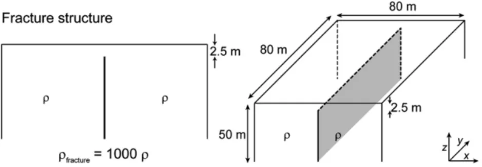
The chosen synthetic structure is shown in Fig. 2, reflecting a verti-cal fracture. The contrast between the fracture (_ρfracture) and the hostrock (ρ) resistivities was set to 1000. In field situations, fractures can be conductive or resistive. Simulations have been led in both ways and nearly led to the same results. Hence, simulations presented here are only with resistive fractures. A superficial top-layer thickness of 2.5 m, covering the hostrock and the fracture resistivity was defined with the same resistivity as the hostrock. The thickness of the fracture is 0.2 m (Fig. 2).

This structure was discretised into quandrangularfinite-elements, with horizontal and vertical extensions of 0.2 m and 0.5 m, respec-tively. The dimensions of the 3D domain is 80 m × 80 m × 50 m (Fig. 2).

3.2. Profiling

The three arrays were numerically simulated on the synthetic structure in profiling mode. Due to symmetry, all three arrays lead to zero potentials when they are parallel to the fracture (see Szalai et al., 2002). Additionally, Sna leads to zero potentials when the array is perpendicular to the fracture, as will be developed more in detail in the next section. Therefore, the profile direction was always chosen perpendicular to the structure with an array offset of 45°, as shown on Fig. 3. Simulation of the signals along the profile was done with a step of 1m and an array length AL of 10 m.

Fig. 4 shows the numerical results of the three null-arrays along a 20 m long profile crossing the vertical fracture at the centre of the pro-file. The resistivity values, as mentioned earlier, reflect the strength of the signals rather than real resistivity values and are obtained by using the respective equivalent geometric factors shown in Fig. 1.

For the MAN (Fig. 4a), the position of the fracture is localised by the inflexion point of the curve at a theoretical value of zero. For both Wγna and Sna, the position of the fracture is given by the maximum of the peak, shown in Fig. 4b and c, respectively. An analysis, carried out by Szalai et al. (2004), on the effect of a varying top-layer thickness

showed that the MAN array yields stronger signals than the Wγna for deeper-lying structures.

In the field, only absolute values can be measured due to

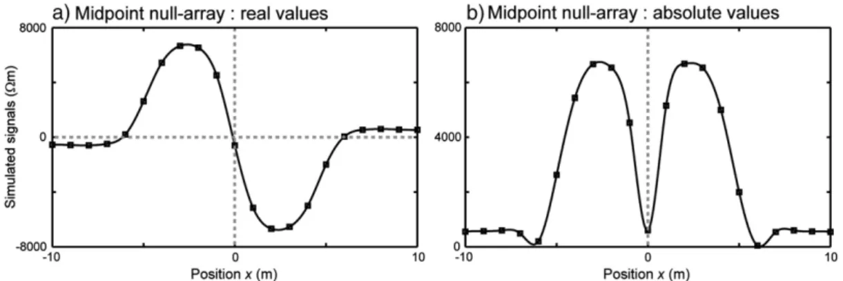
equipment-related constraints. This implies for the MAN, as shown in Fig. 4a and repeated in Fig. 5a, that the structure will be localised be-tween two symmetrical peaks, as shown in Fig. 5b, and not at the in-flexion point.

3.3. Azimuthal measurements

In order to analyse the performance of the three null-arrays in identifying the orientation of the fracture structure, three positions with respect to the fracture have been tested: i) directly above the structure, at 0 m, ii) perpendicularly slightly displaced by 2 m, and iii) perpendicularly displaced by 4 m. For a given electrode spacing, the layout is step-wise rotated around the central point of the array. In our analysis, the rotation was done by 15°, leading to a total of 12 measurements for each electrode configuration. The total rotation was completed by taking into account the symmetry of the arrays.

Fig. 6 shows the simulation results for the classical Schlumberger array (Fig. 6a, b and c) and the three null-arrays with the centre of the array exactly on the fracture (Fig. 6d, g and j), at a distance of 2 m (Fig. 6e, h and k) and at a distance of 4 m (Fig. 6f, i and l), mimick-ing the fact thatfield measurements will most likely not be done ex-actly on the structure.

For the classical Schlumberger array a distortion of the elliptic shape of the situation directly above the fracture (Fig. 6a) can be ob-served for the slightly displaced position (Fig. 6b and c). In some cases the direction of the main axis may be rotated by 90° which could lead to misinterpretation. Additionally, the strength of the signal decreases drastically as soon as the measurements are not done exact-ly above the structure. These two aspects render interpretation of the classical Schlumberger array uncertain in terms of identification of the fracture orientation in cases where measurements are not taken di-rectly above the fracture.

For symmetry reasons, the signal of the MAN is always zero direcly above the structure (Fig. 6d). However, when it is not centred on the structure, the minimum axis of the ellipse yields its direction. For real-world situations the MAN therefore appears to be an appropriate

Fig. 3. Plan-view of the configuration of the Schlumberger null-array (Sna) profile with respect to the direction of the profile (stippled line) and to the fracture (bold grey line). The array is moved step-by-step along the profile. The linear arrays were performed with the identical array line direction.

array to identify the fracture orientation, since it is very unlikely to carry out measurements exactly above a structure.

For the Wγna, when located directly above the structure, shown in Fig. 6g, it is possible to determine the direction of the fracture defined by the symmetry axis perpendicular to the two lobes. On the other hand, when displaced with respect to the structure, as shown in Fig. 6h, four lobes appear with two symmetry axis. Although the frac-ture strucfrac-ture in this case coincides with the a slightly longer symme-try axis, this may change in another situation (Fig. 6i). Therefore, it is not possible to unambiguously identify which of the two axes reflects the fracture orientation.

For the Sna, the situation is similar to the Wγna with four lobes (Fig. 6j) yielding two possible fracture orientations. As opposed to W_{γna with four lobes, the two Sna symmetry axes are defined by} the directions of the zero values. These zero values are due to the rec-iprocity principle (Lanczos, 1961; Van Nostrand and Cook, 1966) as current electrodes are perpendicular to the potential electrodes. Fig. 6j shows the signals for the Sna directly above the structure whilst Fig. 6k and l is slightly displaced, respectively. This array is able to identify the fractures's direction independently of the distance from the structure.

Amongst the presented arrays, the MAN is therefore the most ap-propriate one to determine the fracture's direction quite precisely in-dependently from the distance from the structure.

In thefield however there are often no isolated fractures, but a whole series of them. As a consequence, the phenomenon of the so-called anisotropy paradox (Keller and Frischknecht, 1966; Taylor and Fleming, 1988) plays a role. It results in the rotation of the diagrams by 90°, i.e. the direction of the fracture will be described by the long axis of the ellipse, not by the short one, for both the MAN and the Wγna. The situation is otherwise similar for the classical Schlumberger

array (Taylor and Fleming, 1988). The explanation and the implications of the anisotropy paradox and its conditions will be discussed in a sep-arate paper.

4. Field application

The aim of thefield application was to test and validate the results of the numerical analysis in a setting, where the geological fractures could also be mapped. Hence, the position and the orientation of the fractures could be cross-validated and compared with the results from the geophysical survey which was carried out during a fortnight. After a brief description of the methods, the setting and thefield setup are described. Then, results from classical geophysical investiga-tions, comprising electrical resistivity tomography, classical array pro-filing and very low frequency electromagnetics VLF-EM (e.g. Müller et al., 1995) and VLF-Grad (Bosch, 2002) are presented, leading over to thefield results for the null-array profiling and azimuthal measure-ments. The differentfield approaches are then compared and discussed with respect to their performance in fracture characterisation. 4.1. Methodology

The equipment used in thefield consisted of two different devices: a) a SYSCAL Junior Switch 72 (IRIS instruments), used for the ERT and null-array profiles and b) a VLF-receiver with a VLF-EM antenna and VLF-Grad antenna (J. Duperrex; Chateau d'Oex, Switzerland). 4.1.1. ERT and null-array instrumentation

ERT measurements were carried out using 72 steel electrodes and four multi-core cables with a maximum electrode spacing of 5 m. ERT was performed with both dipole–dipole and Wenner arrays for

Fig. 5. Synthetic example illustrating the transformation from (a) theoretical values to (b) absolute values for the data set corresponding to Fig. 4a.

Fig. 4. The null-array signals over a fracture localised at position 0 m: a) midpoint null-array (MAN), b) Wenner-γ null-array (Wγna) and c) Schlumberger null-array (Sna). Array length (AL) is 10 m and profile steps 1 m.

two electrode spacings, 1 m and 2 m. ERT profiles with 2 m electrode spacings were performed on a 142 m-long profile. The precision of the potential measurement and the accuracy of the resistivity are ~ 0.5%. Potentials up to 400 V and currents up to 1.25 A were applied during

measurements, and corrected for self-potential. ERT acquisitions were performed with 3 to 6 stacks with a cycle time of 500 ms.

For the null-array profiles, the device adapts the potential in the range of 5–400 V, by varying the injected current (~20 mA). Depending

Fig. 6. Classical and null-arrays azimuthal diagrams for two positions to the fracture: classical Schlumberger at a) 0 m, b) 2 m and c) 4 m, midpoint null-array (MAN) at d) 0 m, e) 2 m and f) 4 m, Wenner-γ null-array (Wγna) at g) 0 m, h) 2 m and i) 4 m, Schlumberger null-array (Sna) at j) 0 m, k) 2 m and l) 4 m. External values give the apparent resistivity of the outer circle, whilst the centre is zero for null-arrays. For the classical Schlumberger array, the centre value is given. Direction of the fracture is 0°. Array length is 10 m for all arrays.

Fig. 7. Les Breuleux's quarry situated in the Jura, north-western Switzerland. Black line indicates the 70 m-long profile P1 (0m is on the eastern side). Grey line shows the direction of the major fracture at 30 m on P1, cropping out in the quarry. Positions A1–A5 reflect azimuthal measurement positions. Top right photo shows the quarry wall below the profile. Reproduced by permission of swisstopo (BA12058).

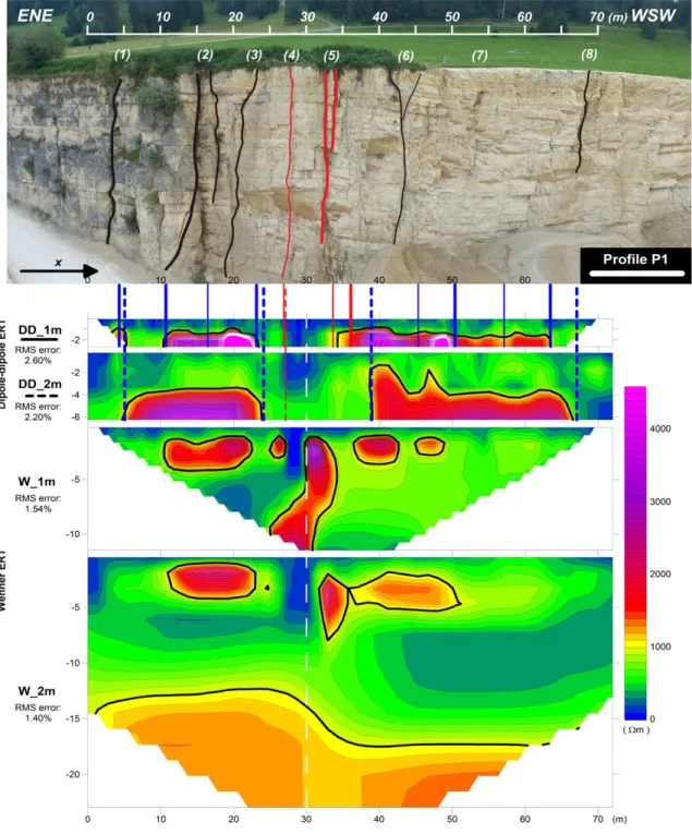
Fig. 8. Top photo: Les Breuleux quarry wall with indicated steep fracture structures (black lines). Red lines indicate the main fracture at about meter 30 along P1. Lower graphs: results from ERT survey: bold lines show transition zones in the limestone below the soil cover detected by dipole–dipole 1m electrode spacing array (DD_1 m), dashed lines indicate transition zones detected with the dipole–dipole 2 m electrode spacing array (DD_2 m), white line indicates detected zones corresponding to the main anomaly at 30 m, also detected by Wenner tomographies, W_1 m and W_2 m (white dashed lines). Contour interval of iso-values 200Ωm.

4.2. Field setup

The Breuleux quarry, located in the Jura mountains (Switzerland) was chosen as thefield test site (Fig. 7). In this quarry, outcrops of Ju-rassic massive limestones of the Jura fold and thrust belt are well ex-posed on the 25 m high quarry wall. The quarry has been excavated within a fold with an axis of about N80°. The limestones exposed in the quarry are crosscut by several sub-vertical fractures and overlain by a soil cover (top right photo, Fig. 7). The geometry of the structures in this quarry reflects a whole series of steep fractures, similar to the synthetic structure used for the numerical analysis (Fig. 2). Eight frac-ture families (1)–(8) were mapped on the quarry wall (Fig. 8). The thickness of the lines drawn on the discrete fractures are related to the fracture aperture and persistence.

The black line in Fig. 7 shows the 70 m long east–west oriented pro_{file P1 which was investigated with the different geophysical} methods. The profile and its approximate projected scale are indicated on the photo at the top right of Fig. 7. The projection of the geophysical results onto this profile may lead to a positioning error of 2–3 m. Posi-tions of azimuthal measurements (Fig. 7) were defined from the re-sults of the profiling measurement, in order to be located between two fractures (A1), close to a major fracture (A2 and A3), and directly above the fracture (A4 and A5).

4.3. Results of geophysical pro_{filing investigations}

In order to obtain as much information as possible, measurements along the pro_{file P1 were done with multiple classical geophysical} methods as well as with the null-array configurations. In the follow-ing, the results of the electrical resistivity tomography (ERT) arefirst presented, followed by the results derived from classical profiling measurements, leading over to the null-array profiling results. 4.3.1. Electical resistivity tomography (ERT)

The results of the Wenner ERT shows roughly two layers: an over-laying conductive one of 10 to 15 m thickness and a more resistive lower layer (Fig. 8). A conductive anomaly appears at ~ 30 m, at a depth between 2 and 10 m (Fig. 8). This anomaly corresponds to the major fracture that crosscuts the quarry (cf. Fig. 7). A step is observed at the interface between the two layers in the Wenner 2 m ERT profile (Fig. 8).Dipole–dipole ERT is known to be more sensitive than Wenner ERT to vertical structures. The sensitivity to lateral heterogeneity is

clearly shown in Fig. 8 for the two dipole–dipole ERT, whilst the inves-tigation depth is smaller than for the Wenner ERT. The main anomaly detected with the Wenner ERT at 30 m is still the most pronounced, but additional anomalies appear too. Secondary fractures are also detected by the dipole–dipole ERT (blue lines in Fig. 8).

4.3.2. Classical profiling methods

Classical geoelectrical and electromagnetic measurements were carried out for cross-validation and comparison purposes. A profile along P1 was carried out with the classical Schlumberger array with two array lengths (AL), 10 and 20 m with measurement steps of 1 m: one pro_{file with the array in the same direction as P1 (in-line} measurement), and one profile with the array perpendicular to P1 (offset measurement). The results of the classical geoelectrical and electromagnetic profiles along P1 are shown in Fig. 9.

The only clear feature identified by the Schlumberger profile parallel to P1 (by coinciding minimas for both electrode spacings) is the main fracture at 30 m, being coherent with the ERT measurements (Fig. 9a). On the profile perpendicular to P1, the fracture at 30 m is characterised by two clear minima (Fig. 9b). As for the dipole–dipole ERT, other anomalies (black stars in Fig. 9b) can be identified. The VLF curves shown in Fig. 9c and d only reveal the main anomaly at about 30 m on the profile P1. It corresponds to the inflexion point for the VLF-EM (Fig. 9c) and to the peak maximum for the VLF-Grad (Fig. 9d). This prominent anomaly, also detected by all classical electrical methods, is the only feature that both VLF methods detected. This can be explained by a far higher resistivity contrast and/or width and vertical extension. 4.3.3. Profiling with null-arrays

According to the numerical analysis, all three presented null-arrays are capable of detecting the position of fractures in the profiling mode, yielding strong signals (Fig. 4). For Sna and Wγna, the position of the fracture is defined by the maximum of the peak, whilst for the MAN array the fracture is theoretically de_{fined by the minimum between} two symmetrical peaks (Fig. 5).

Field data for null-arrays data along P1 are shown in Fig. 10 togeth-er with the data retrieved from the classical methods. All null-array profiles were carried out for two electrode spacings, 10 m (dashed lines) and 20 m (full lines), with a measurement step of 1 m. The angle offset between the direction of the profile P1 and the array axis was approximately 45°. Only anomalies detected by both array

lengths were considered. The MAN profile along P1 reveals one

Fig. 9. Results of classical geophysical profiles along P1: classical Schlumberger profile a) with array parrallel to P1 and b) with array perpendicular to P1, for two electrode spacings (10 m and 20 m); c) VLF-GradΔHy (%, amplified by a factor); d) VLF-EM quadrature Hz/Hy (%). Classical Schlumberger profiles lead to apparent resistivity values (Ωm). Dashed lines indicate the near-surface measurements (array length 10 m for Schlumberger profiles and 183 kHz frequency for VLF profiles), full lines for deeper investigation depth (array length 20 m and 23.4 kHz frequency). Grey stars indicate main anomaly at 30 m detected by the given methods. Black stars indicate minor anomalies.

prominent anomaly corresponding to fractures (4) and (5) (Fig. 10a). Two other anomalies are also detected towards the WSW (Fig. 10a). The Sna profile also identifies the main fractures (4) and (5), as well as four other anomalies correlating with quarry fractures (Fig. 10b). The amplitude for the electrode spacing 10 m was exaggerated by a factor 2.

The Wγna profile distinguishes eight anomalies (Fig. 10c). Five of them are prominent, with sharp and high peaks, including two attrib-uted to the main fractures (Fig. 10c). Three minor anomalies correlate well with the observed geological fractures (Fig. 10c).

The fracture zones (4) and (5), characterised by a mapped vertical displacement, are detected with all profiling methods (Fig. 10). More-over, as all observed fractures were identified with Wγna, this array seems to be the most appropriate for fracture localisation.

4.4. Azimuthal measurements with null-arrays

Fourteen azimuthal measurements were performed at_{five different} positions (Fig. 7). The positioning was done in accordance with the geo-logical mapping, which also included mapping of the orientation of the fractures: position A1 located between fracture zones (1) and (2), A2 lo-cated near to fracture zone (5), A3 slightly displaced from the position of A4, located above the major fracture zone (5) and A5 another location to study the effect of mispositioning close to A4. In accordance with the nu-merical simulation, measurements were carried out every 15° around the central point of the array.

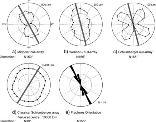
As an example of results, Fig. 11a–c show the azimuthal diagrams obtained at the position A4 for all null-arrays, yielding a fracture orienta-tion of 150°–165°. The shapes of the measured diagrams are in very good

Fig. 10. Photo of the quarry wall with numbered mapped fractures (black lines) and main fractures (red lines). Profiles of null-arrays carried out with electrode spacings 10 m (dashed lines) and 20 m (full lines): a) midpoint null-array (MAN), b) Schlumberger null-aray (Sna), c) Wenner-γ null-array (Wγna); d)–g) correspond to the profiles shown in Fig. 9. Stars show anomalies detected by the given methods. The red stars highlight the signals related to the major fracture at 30 m, the blue stars indicate other detected fracture zones. The grey ellipses group anomalies which can be assigned to corresponding geological features, indicated with arrows. The dashed ellipse corresponds to the wide fractured zone (7).

accordance with the numerical analysis if the anisotropy paradox is taken into account (Fig. 6). Fig. 11d shows the azimuthal diagrams mea-sured at position A4 with the classical Schlumberger array. According to Keller and Frischknecht (1966), if the anisotropy paradox occurs, the long axis of the ellipse on polar diagrams should be parallel to the frac-ture, e.g. N30° in that case. Fig. 11e represents the rose diagram of all the fracture orientations measured on the quarry wall, where the orien-tation of fracture zone (5), i.e. 150°, high-lighted as a stippled line, is in very good accordance with the azimuthal measurements.

Fig. 11a shows the diagram for the MAN, yielding a fracture orienta-tion of 150°, normal to the well-defined minimum orientation. Fig. 11b shows the diagram of Wγna. In this case, the direction with its major axis being N165° corresponds to the fracture orientation. Fig. 11c shows the diagram for the Sna measurements, yielding two possible fracture orientations, N165° or N75°. The classical Schlumberger array does not seem in accordance with other measurements. Since the orien-tations derived from Sna have a higher accuracy than the other arrays, combining them with the MAN will allow the choice of the correct orientation.

Table 1 shows the summary of all azimuthal data results. All mea-surements lead to a very similar orientation, between 150° and 165°, which are in good agreement with the geological measurements (Fig. 11e).

In some cases, interpretation of the azimuthal diagram is not straight-foreward, possibly due to near-surface effects on the mea-sured signal. But even in such cases, it is possible to evaluate the orien-tation of the fracture. As an example, Fig. 12 shows the azimuthal diagrams of the Sna at position A2 (Fig. 12a with array length 20 m and Fig. 12b with 10 m array length). It reveals that the distortion of the theoretical shape is most likely the consequence of a measuring error (at 45° and its pair at 225° in Fig. 12b). However, the real fracture orientation is still identified by the clear minima (at N150°).

4.5. Discussion offield measurements

Thefield measurements have shown that null-arrays have a con-siderable potential in detection of the position and orientation of frac-tures, correlating in most cases with the numerical analysis.

As shown in Fig. 10, null-array profiles are far more sensitive to a va-riety of fractures at different scales than VLF profiles which only detected the major fractures. The Wγna was found to be the most sensitive of all methods. Of the classical geophysical methods, the Schlumberger array perpendicular to the profile proved to be the most sensitive with respect

Fig. 12. Azimuthal diagrams obtained at position A2 with Schlumberger null-array (Sna) illustrating the possible distortion offield measurements diagram with respect to the the-oretical analysis for two electrode spacings: a) array length 20 m; b) array length 10 m. Table 1

Orientations obtained from azimuthal measurements with the three null-arrays at dif-ferent positions on profile P1 (except for A5). Results given as a range indicate a lack of measurement accuracy. Name A1 A2 A3 A4 A5 Position 12 m 26 m 28 m 30 m 30 m, 2 m South MAN AL = 10 m N150° N150° N165° Wγna N165° Sna N165°–150° N150° N165° MAN AL = 20 m N150° N150°–165° N150°–165° Wγna N165°–150° Sna N130°–150° N165° N165°

Fig. 11. Azimuthal measurements at position A4 on profile P1 with an array length of 20 m: a) midpoint null-array (MAN), b) Wenner-γ null-array (Wγna), c) Schlumberger null-array (Sna), d) classical Schlumberger array. e) Rose diagram representing the strike of the fractures in the quarry. Measured orientations are written below.

the required depth. Ideally, the array length should be similar or slightly bigger than the distance between main fractures. Infield situ-ations, where this distance is typically not known, it is recommended to carry out the same profile with at least two distinctly different array lengths in order to identify the optimal size.

The investigation depth for null-array measurements is dif_{ficult to} determine. It is expected that they are at least sensitive to shallow fractures. Since no inversion of data is carried out, more precise eval-uation of the investigation depth is not possible.

For azimuthal measurements, a step-wise rotation of 15° seems to be a good compromise between accuracy, given by the number of data points and efficiency.

For profiling with null-arrays in the field, the Wγna is the most recommended array, although results from Sna are also satisfactory. The major disadvantage of the Sna, in addition to its lower sensitivity is related to its implementation in thefield, requiring twice as much time to perform a profile than for the Wγna.

For azimuthal measurements, the MAN yields a unique but less precise orientation allowing to chose between the two more precise perpendicular directions determined by the Sna.

5. Conclusions

This study has shown that geoelectrical null-arrays are a powerful tool for the characterisation of fractures, comprising localisation and determination of orientation. Three null-array methods were investi-gated, in profiling and azimuthal modes, first in a numerical analysis, followed by afield application.

In the profiling mode, the numerical analysis revealed that the posi-tion of the fracture for both Wγna and Sna coincides with the maximum of the peak, allowing very precise localisation. For the MAN, the position of the fracture is localised by the in_{flexion point of the curve at a} theo-retical value of zero, rendering identification more delicate. The results from thefield profiles revealed that the Sna detected more fractures than the MAN, but the Wγna was the only null-array capable of localising all the observed fractures. All classical geophysical methods applied in thefield were only able to detect the major fracture zone but none of them was capable of detecting the minor fractures. Hence, the use of null-arrays, in particular the Wγna, which has been rarely used so far, has proved to be a powerful method in thefield for charac-terisation of fractures.

In the azimuthal mode, the numerical analysis resulted in typical polar diagrams for each null-array. They revealed two possible orienta-tions of a fracture perpendicular to each other for the Sna and the Wγna, whilst the MAN array yields a unique solution. However, the orienta-tions derived from Sna have the highest accuracy. Thefield results, car-ried out at different positions with respect to the major fracture zone, yielded polar diagrams mostly in very good accordance with the nu-merical analysis. The orientation of the fracture was best determined by combining the Sna with the MAN: the MAN allowing the choice of the correct orientation given with the best precision by the Sna.

In summary, the Wγna is the most appropriate and efficient for the profiling mode, whilst the combined use of MAN and Sna yields the best results for the azimuthal mode infield situations. The MAN is easy in its implementation, allowing evaluation of the orientation.

still has to be investigated. However, the presented results show that geoelectric null-arrays can play an important role in characterising fractures.

Acknowledgments

We gratefully acknowledge Prof. Christian Hauck and the Universi-ty of Fribourg for lending the geophysical device and for fruitful dis-cussions. Thanks to the physicist Lucien Falco for the assistance during thefield work. The careful reviews and conspicious comments by Dr. Markus Gurk were highly appreciated.

References

Bogolyubov, N.P., 1984. Guide to Interpreting Two-component Modified VES. Stroyizdat, Moscow (In Russian).

Bosch, F., 2002. Shallow depth karst structure imaging with the Very Low Frequency-Electromagnetics Gradient (VLF-EM GRAD) method: a new geophysical contribution to aquifer protection strategies compared with other near surface mapping geophysics. PhD Thesis. University of Neuchâtel.

Edwards, L.S., 1977. A modified pseudosection for resistivity and induced-polarization. Geophysics 42 (5), 1020–1036.

Keller, G.V., Frischknecht, F.C., 1966. Electrical Methods in Geophysical Prospecting. Pergamon Press.

Lanczos, C., 1961. Linear Differential Operators. Van Nostrand, New York.

Loke, M.H., 2012. Tutorial: 2-D and 3-D electrical imaging surveys. Copyright (1996-2012). Available via http://www.geotomosoft.com/downloads.php (Accessed 8 September 2012).

Marescot, L., 2004. Modélisation directe et inverse en prospection électrique sur des struc-tures 3D complexes par la method des elementsfinis. Thèse de Doctorat. Université de Nantes.

Müller, I., Stiefelhagen, W., Intchi, A.R., 1995. Réflexions sur les résultats obtenus par l'enregistrement en continu des paramètres géophysiques, électromagnétiques (VLF-EM) et magnétiques, pour l'exploration hydrogéologique des aquifères karstiques (Grotte de Milandre, Jura Suisse). Bulletin de la Société Neuchâteloise de Sciences Naturelles 118, 109–119.

Parker, L.R., 1984. The inverse problem of resistivity sounding. Geophysics 49, 2143–2158. Roy, A., Apparao, A., 1971. Depth of investigation in direct-current methods. Geophysics

36 (5), 943–959.

Szalai, S., Szarka, L., 2006. Parameter sensitivity maps of surface geoelectric. ICEEG, Wuhan, Chine, Geophysical Solutions for Environment and Engineering, vol. 1. Science Press USA, Inc. 260–264.

Szalai, S., Szarka, L., 2008a. Parameter sensitivity maps of surface geoelectric arrays. Part 1: linear arrays. Acta Geodaetica et Geophysica Hungarica 43, 419–437. Szalai, S., Szarka, L., 2008b. Parameter sensitivity maps of surface geoelectric arrays. Part

2: nonlinear and focussed arrays. Acta Geodaetica et Geophysica Hungarica 43, 439–447.

Szalai, S., Szarka, L., 2008c. On the classification of surface geoelectric arrays. Geophysical Prospecting 56, 159–175.

Szalai, S., Szarka, L., 2011. Expanding the possibilities of two-dimensional multielectrode systems, with consideration to earlier geoelectric arrays. Journal of Applied Geophysics 75 (1), 1–8.

Szalai, S., Szarka, L., Prácser, E., Bosch, F., Müller, I., Turberg, P., 2002. Geoelectric mapping of near-surface karstic fractures by using null-arrays. Geophysics 67, 1769–1778. Szalai, S., Szarka, L., Marquis, G., Sailhac, P., Kaikkonen, P., Lahti, I., 2004. Colinear

null-arrays in geoelectrics. IAGA WG 1.2 on Electromagnetic Induction in the Earth. Tarkhov, A.G., 1957. On electric geophysical exploration methods of a pure anomaly.

Izvestya Akademii Nauk SSSR. Seriya Geofizica 8, 979–989.

Taylor, R.W., Fleming, A.H., 1988. Characterizing jointed systems by azimuthal resistivity surveys. Ground Water 26, 464–474.

Van Nostrand, R.G., Cook, K.L., 1966. Interpretation of resistivity data. Geological Survey Professional Paper 499.US Government Printing Office, Washington DC. Winter, H., 1994. Tensor-Geoelektrik an der Kontinentalen Tiefbohrung. Fortschrittberichte,