Tissue segmentation on MR images of the brain by possibilistic clustering on a 3D wavelet representation

Original Research

Tissue Segmentation on MR Images of the Brain by

Possibilistic Clustering on a 3D Wavelet

Representation

Vincent Barra, PhD,

and Jean-Yves Boire, PhD

ACCURATE MEANS OF QUANTIFYING the volume of brain tissues in diseases such as Alzheimer’s dementia, epilepsy, or hydrocephalus would be most useful for diagnosis, treatment, and general understanding. Bezdek et al (1) have reviewed some MR segmentation techniques using pattern recognition, making a distinc-tion between supervised and unsupervised methods.

Supervised methods need crisp labels for some im-ages, so the set of images to be analyzed is partitioned into a training set and a test set. This class of methods includes parametric algorithms [modeling of the image by Markov or Gibbs random field (2,3), Bayes’ classifier with estimation of the parameters by maximum likeli-hood expectation (MLE) (4)], nonparametric algorithms [k-nearest neighbors (k-NN) (5)], neural networks (NN) (6), and other original algorithms (7). Supervised meth-ods can be highly dependent on choices of training sets. Clarke et al (8) compared MLE, k-NN, and NN and con-cluded that the difference in segmentation is small when tissues are well differentiated by the

tissue-spe-cific MR parameters. For tissues that are not well sep-arated, such as gray matter (GM) and white matter (WM), they observed differences in segmentation be-tween MLE and k-NN/NN because a specific statistical model is assumed for MLE that does not necessarily suit the data. More generally, the literature reports that small differences in operator judgment may cause wide variations in results, making these methods unsuitable for quantitative analysis when data validation training is defective (9).

The other group of MR segmentation techniques com-prises unsupervised methods. They process an image with no learning, and set out to group voxels in the image in a known number of clusters that ultimately must be assigned physical tissue labels. The two main approaches are hard and fuzzy clustering, which aim at separating features in different clusters by minimizing an objective function (10). Hard clustering produces a partition so that each voxel receives a unique tissue assignment. In contrast, a fuzzy clustering algorithm allows features to belong to more than one class, with certain degrees of membership. This latter technique has been widely used for MR image segmentation (11). Brandt et al (12) used this method for the calculation of GM, WM, and cerebrospinal fluid (CSF) volumes in hy-drocephalic children. Philipps et al (9) used a fuzzy clustering algorithm to segment diagnostically relevant tissue contrast information in MR images of hemor-rhagic glioblastoma multiforme. Clark and al (13) combined fuzzy clustering and knowledge-based tech-niques to identify abnormal tissues. Other unsuper-vised methods exist, such as fractal analysis (14), in which tissues are distinguished by comparing their fractal dimensions on MR-weighted images.

When one of these techniques is to be used to seg-ment MR images, relevant features have to be chosen for the clustering. MRI is a multispectral imaging tech-nique able to provide several different parameters and thus features. The first feature that can be exploited is the signal itself, mainly by means of T1-, T2-, and pro-ton density-weighted images. This information is widely used for tissue segmentation (6,9,12,15) but is highly sensitive to instrumental variations of the NMR signal and also assumes that more than one image can be obtained from the protocol and that the images are Faculty of Medicine, ERIM, 63001 Clermont Ferrand Cedex, France.

Contract grant sponsors: Med, France and the Segami Corporation. *Address reprint requests to: V.B., Faculty of Medicine, ERIM, 28 Place henri Dunant, BP 38, 63001 Clermont Ferrand Cedex, France. E-mail: vincent.barra/j-yves.boire@u-clermont1.fr

Received March 24, 1999; Accepted November 3, 1999.

perfectly registered. MRI also allows the computation of parametric imaging, so that NMR parameters such as T1, T2, or proton density are available for each voxel. These parameters are closely related to physical and chemical properties of tissues and are less sensitive to instrumental variations than the signal itself (16). How-ever, the choice of this type of feature is time consum-ing, because the acquisition time may be longer, and postprocessing is needed to compute the NMR param-eters and to register the images. Other features can be computed that use not only the signal but also contex-tual information on voxels. This includes edge informa-tion (11) and texture analysis (17).

Kiviniitty (18) reported for multispectral analysis that T1 and T2 parameters are significant for normal tissue characterization in human brain MR imaging. Just and Thelen al (19) agreed but noted that pathologic entities such as tumors or edema are characterized by wide ranges of parameters (T1-, T2-, proton density-weight-ed). By an analysis of different tumors, they showed that the overlapping of tissue parameters in these en-tities rules out a reliable diagnosis based on a quanti-tative evaluation of this set of parameters alone. Several groups have succeeded in classifying voxels according to a multispectral analysis (6,9,12,15), but few methods effectively cluster the brain tissues with one MR image only. Lim and Pfefferbaum (20) subtracted late echo images from or added them to early echo images of a spin-echo sequence to enhance fluid/tissue and GM/WM tissue contrast, respectively. More recently, Reiss et al (21) segmented GM, WM, and CSF in both single-channel and multiecho MR images with a fuzzy method, by fitting the tissue class histograms with an analytical model composed of multiple normal distribu-tions.

In this paper, we quantify GM, WM, and CSF volumes using a fuzzy unsupervised method on a single se-quence of three-dimensional (3D) MR images from pa-tients suffering from Alzheimer’s disease (22). The pos-sibilistic clustering algorithm (PCA), devoted to the resolution of our clustering problem, is presented first. We then introduce original features to cluster, the wavelet coefficients vectors. We demonstrate their in-terest for our purpose, and we show that the clustering of these features with PCA allows us to separate WM, GM, and CSF in a reliable way. Finally, validation and results of our clustering method are presented.

MATERIALS AND METHODS

Imaging Parameters

MRI was performed using a Siemens Magnetom system (Erlangen, Germany), with a 1 T superconducting mag-net and a head coil. Owing to the constraint imposed by the Alzheimer’s disease patients (risk of claustropho-bia, movement), a fast 3D imaging technique [fast low-angle shot (FLASH) 3D sequence (23)] was used to ac-quire the whole brain volume, maximizing the WM/GM contrast for the chosen acquisition time. Parameter val-ues were TR/TE 50/10 msec and flip angle 35°, giving us T1-weighted images with a Pelc angle (24). The total acquisition was less than 7 minutes. The reconstructed

volumes were 128 ⫻ 128 ⫻ 64, with 2 ⫻ 2 ⫻ 2 mm3

voxels. Skin and skull were removed using a polar transform (20), to process the clustering on the brain tissues alone.

Possibilistic Clustering Algorithm

Hard approaches to unsupervised classification are generally based on the determination of a crisp parti-tion of a set of vectors into C classes. It is assumed that a feature vector belongs to one and only one class. Di Gesu and Romeo (25) discussed MR segmentation us-ing four crisp clusterus-ing algorithms and concluded that this approach is ill suited when clusters overlap or when the information is unclear and uncertain. MR images of human brain display both of these character-istics: for example, the boundary between GM and WM is blurred or fuzzy and uncertainty arises from noise, partial volume effect, or anatomical variations within “pure” tissue compartments. Hence we applied fuzzy clustering, issuing from fuzzy logic (26), and particu-larly the PCA (cf. Appendix). Fuzzy clustering in medical images seems to have been first attempted by De La Paz et al (27); to our knowledge, this is the first time PCA has been used for clustering MR data on a single brain volume.

The bases of our clustering algorithm were the same as those found in Krishnapuram and Keller (28). We nonetheless brought significant original improvements to this method with respect to our particular problem: 1. Krishnapuram and Keller (28) used a fixed value for the parameter that controls the degree of fuzzi-ness (m⫽ 2), whatever the problem. We, however, created a specific method to estimate the “best” m that suited our data.

2. The same authors used PCA in a context of com-puter vision (random image, line, or circle detec-tion). The chosen features were the spatial coordi-nates of the points, and the distance d determined the shape of the clusters. We addressed a more complex clustering problem and we thus intro-duced original features, the wavelet coefficients vectors, which used the information from single MR images most efficiently.

Value of m

The parameter m controls the degree of fuzziness of the resulting fuzzy maps (cf. Appendix). If m is close to 1, the partition generated by PCA is almost crisp, and memberships become fuzzier as m increases. When m tends to infinity, all the memberships for a given voxel are equal to 1/C. There is no optimization process to compute the “best” m; it greatly depends on the nature of the data. A value of m lying in the interval [1.5,3] is generally accepted. Tucker (29) suggests taking m⬎ N/ (N⫺ 2) to guarantee the convergence of PCA. We pro-pose finding mBin [1.5,5], which gives the “best”

parti-tion of our brains algorithmically.

A trained specialist was requested to label a brain volume according to three types of tissues (GM, WM, and CSF). The resulting labeled image, IREF, was used

to determine mBby applying the following process to

the original image: D⫽ infinity

For m⫽ 1.2 to 5 step 0.1 do the following:

1. Compute the fuzzy partition GMm, WMm, CSFm

generated by PCA.

2. Defuzzyfy the resulting partition to create an im-age, INEW.

3. Compute the difference Dmbetween INEWand IREF

4. If Dm⬍ D, then D ⫽ Dmand mB⫽ m.

End

In the defuzzyfication step, each voxel was assigned to the class for which it had the greatest membership. This produced a labeled image, INEW. The difference Dm:

Dm共INEW,IREF兲 ⫽

冘

i⫽ 1

N ␦i,

where ␦i⫽

再

0 if the class of voxel i in IREF ⫽

the class of voxel i in INEW

1 otherwise

measured the number of wrongly classified voxels.

Distance Measure

The shape of clusters obtained by PCA closely depends on the choice of the distance. If d is the Euclidean distance, the structure of the clusters generated by PCA is spherical. Other measures of distance are available that detect ellipsoidal (30) or hyperspherical (31) clus-ters. Because our parametric space was quite complex (cf. infra: the features), the shape of the clusters was a priori unknown. We therefore applied PCA with the most conventional and the least restrictive distance, the Euclidean one, thus assuming that the clusters in the parametric space were almost spherical.

The Features

The protocol provided us with only one volume per pa-tient. We therefore had to choose relevant feature vectors

that extracted the best information from the MR images. We took into account both signal and contextual informa-tion on voxels by using a wavelet representainforma-tion of the image (32). This representation corresponds to a decom-position of the image into a series of approximations at different scales. What makes it interesting is that each scale provides three images, giving the contrast in a given frequency range and along three particular spatial orien-tations. The resulting information is thus quite localized in space and in frequency, or more precisely in character-istic scale. The decomposition of the MR images with a compressible and computationally efficient wavelet trans-formation, called DAUB4 (33), enabled us to obtain for each voxel V a set of coefficients referred to as the wavelet coefficients of V. At a coarse scale or resolution, the wave-let coefficient gives information on larger structures that provide the image context of V. At a finer resolution, it expresses more precisely the local environment of V in the image. Each coefficient should then express a piece of information on V, from low frequencies to high frequen-cies and in any spatial orientation, hence giving together information both on cerebral structures (first coeffi-cients— or coarser scales) and on textural properties of V (last coefficients— or finer scales).

Figure 1 presents a 3D wavelet representation of a brain slice, using the DAUB4 transform at the third scale, from which the wavelet coefficients are built. In this figure, VHFigives the high vertical frequencies at level i (detection

of horizontal edges), HHFigives the high horizontal

fre-quencies at the same scale (detection of vertical edges), and CHFigives the high frequencies in both directions. Ri

corresponds to the lowest frequency image.

In the following, we choose as a feature to cluster the wavelet coefficients vector (WCC). Any voxel v is thus featured by its set of wavelet coefficients extracted from the wavelet decomposition, from the largest to the shortest scale, and in any spatial orientation.

RESULTS AND DISCUSSION

Optimization of the Parameter m

A FLASH 3D image of a normal brain was segmented by a trained specialist into three crisp classes (GM, WM, Figure 1. Decomposition of an MR slice of the brain with the 3D Daubechies wavelet transformation at level 3.

and CSF). This image was clustered with PCA and the wavelet coefficients vectors for values of m in the inter-val [1.5;5]. The percentage of misclassification was computed as a function of m (Fig. 2). This plot reveals that any value of m ranging in the interval [1.5;3] gave a low value for Dm, leading to an average of 4.5% of

misclassification in the encephalon. The abrupt change in the value of Dm(m) for m ⫽ 3.0 corresponds to a

fusion of the GM and CSF classes in the clustering process, leading to several voxels being wrongly classi-fied as CSF, whereas they actually belonged to GM. M⫽ 2.4 was taken as the value of the parameter thereafter.

Validation on a Simulated MR Brain

A computerized brain phantom developed at the McConnell Brain Imaging Center (Montreal Neurologi-cal Institute, McGill University) (34) was used. The an-atomical model consisted of a set of 3D fuzzy tissue membership volumes, one for each tissue class (WM, GM, CSF, subcutaneous fat, muscle, skin, and skull). The voxel values in these volumes reflected the propor-tion of tissue present in that voxel. Volumes were de-fined at a 1 mm isotropic voxel grid in Talairach space. This model was used to generate realistic simulated MRI volumes.

Several T1-weighted simulated MR images (Vol1,. . .Vol8) of the same brain were created, varying in

their slice thickness ST (1, 3, or 5 mm), their additive noise (AD; expressed as a percent standard deviation relative to the mean signal intensity for a reference brain tissue), and their radiofrequency (RF) inhomoge-neity. The noise model was created by taking into ac-count image parameters, with white Gaussian noise added to quadrature components of the received signal. The RF inhomogeneity was simulated using fields re-covered from real scans and scaled for different percent sensitivity ranges (34). We clustered these images with PCA and the wavelet coefficient vectors as features.

All the tissue maps were fuzzy and absolute, i.e., the gray level of each voxel in a tissue map was the

mem-bership of the voxel for that tissue. To compare our tissue maps with the one provided by (34), a “fuzzy volume” was first computed for all tissues I, given by

Vi⫽

冉

冘

j⫽ 0

Nb voxels uij

冊

where v is the volume of one voxel in the image. A labeled image, created by assigning each voxel to the tissue class for which it had the greatest membership, was moreover compared with the reference labeled im-age of the McConnell brain by means of the Tanimoto coefficient (35). This index was proposed for comparing two segmentations in a more critical way than compar-isons using the volumes. It is defined for a given voxel tissue assignment as the number of voxels that have this tissue assignment in both segmentation simulta-neously divided by the sum of voxels where either seg-mentation has the tissue assignment. The index is close to 1 for very similar results and is near 0 when the labeled images share no similarly classified voxels. Ta-ble 1 presents the values of Viand the Tanimoto

coef-ficients for all the Voli.

Volumes Vi were systematically overestimated, what-ever the slice thickness, the RF inhomogeneity, and the additive noise. This was because the memberships gen-erated by PCA were not probabilistic, whereas those provided by Kwan et al (34) were probabilistic. The sum of the memberships for a given voxel i was equal to 1 in Kwan et al (34) but was greater than or equal to 1 for PCA, thereby leading to a greater volume. Nevertheless, memberships exhibited by PCA and WCC were better suited to ambiguous areas than probabilistic ones, as pointed out above.

Also, the McConnell brain provided several other fuzzy maps (glial matter, which misleadingly seemed to be limited to the area of the ependymal layer of the ventricles and not to the whole glial matter, fat, etc.) that were not detected here as separate classes. The

Figure 2. Percentage of misclassification as a function of the parameter m, which controls the degree of fuzziness.

voxels that belong to these fuzzy maps were incorpo-rated in either GM or WM or CSF, thus increasing their total volume, but not significantly.

Finally, the algorithm always detected as GM an in-terface between the lateral ventricle walls and the WM of the corpus callosum. There is no gray matter in this area (36), and the GM detection seemed to be due to the smooth transition in the MR image between the CSF gray level and the WM one. However, the errors in the total WM, GM, and CSF volumes were less than 6% for the 8 volumes. The average relative error for WM vol-ume estimation was approximately 3.3%, for GM less than 1%, and for CSF about 2.8%. The WM overestima-tion was probably because the GM/WM boundary was not well defined, and so some GM voxels (particularly in the cortex) were counted in the WM with small mem-berships. The clustering preserved the existing ambi-guity in these areas by assigning positive memberships to both WM and GM for those voxels. Concerning the labeled images, the estimations of tissue volumes were consistent whatever the noise, RF inhomogeneity, and slice thickness. The Tanimoto indexes were generally high, close to 1 (from 0.76 to 0.89 for GM, from 0.78 to 0.88 for WM, and from 0.74 to 0.89 for CSF). The worst results were obtained for thick slices, with the highest percentages of noise and RF inhomogeneity. These high values could be explained by the fact that PCA mem-berships represent true degrees of belonging, and not degrees of sharing. When taking the greatest member-ship, the best tissue that suited the voxel data was chosen. (cf. Appendix)

Consistent results for volume estimation with respect to slice thickness suggested that PCA tracked changes in partial volume effect.

The effects of RF inhomogeneity were sensitive in the WM map, less sensitive on GM, and not significant on CSF fuzzy maps. For given slice thickness and noise, the WM fuzzy volume varied about 5% when RF inho-mogeneity percentage varied from 20% to 40%, whereas CSF and GM volumes varied about 1% and 2%, respec-tively.

Finally, the presence of noise did not seem to affect the results of the clustering process. Noise actually had a specific frequency signature detected by the wavelet coefficients as different from the brain tissue

signa-tures. Figure 3 illustrates the tissue maps and the la-beled images obtained on two slices.

Clustering on Alzheimer’s Brains

The three slices illustrating the results were chosen because of their tissue particularities. The first one, located on the upper part of the brain, contains several fissures and sulci (precentral and central sulci) that must be detected as belonging to the CSF. The second slice intersects the ventricles and shows structures such as the head of the caudate nucleus, the thalamic nuclei, the putamen, the atrium of the lateral ventricle, and the corpus callosum. The last slice contains basal ganglia (pallidum, putamen, head of caudate nucleus), some sulci and fissures, the third ventricle, and the temporal horn of the lateral ventricle, thus providing a wide variety of tissues. PCA with the wavelet coefficients vectors as features never failed to produce segmenta-tion maps, which then needed to be validated.

Clustering of a FLASH 3D Volume

The clustering process on the wavelet coefficients was applied with four classes to detect GM, WM, CSF, and the background in the Alzheimer’s images (Fig. 4). Any number of further classes can be added to detect ab-normal tissues. Accurate quantitative evaluation of MR image segmentation is practically impossible because the true tissue that each image voxel belongs to is unknown. Few studies have been performed to validate volume measuring techniques because of the difficulty in obtaining in vivo anatomical specimens from sub-jects and segmenting them appropriately in vitro. Five normal brains (S1–S5), aged 22, 25, 30, 44, and 63 years, and five Alzheimer’s brains (A1–A5), aged 67– 84 years, were clustered to assess our segmentation. The numbers of voxels assigned to CSF and the GM/WM ratio on the defuzzified image were processed. These figures were then compared (Table 2) with those found by Matsumae et al (37) and Miller et al (38).

Matsumae et al (37) determined the changes with age of the brain and CSF volumes in 49 normal volunteers aged 24 – 80 years. In particular, they computed a rel-ative CSF volume as a percentage of the intracranial Table 1

Comparison of Fuzzy Tissue Volumes and Labeled Images Between PCA and Reference 34* MR data set MR image parameters Fuzzy volumes[Vi(cm

3_{)] Tanimoto coefficients} RF (%) ST (mm) AD (%) WM GM CSF WM GM CSF Reference values 567.3 585.6 229.6 1 1 1 Vol1 20 1 3 580.1 589.6 232.1 0.89 0.88 0.88 Vol2 20 1 7 578.7 590.1 232.8 0.88 0.83 0.83 Vol3 20 3 3 587.1 587.1 237.1 0.85 0.86 0.89 Vol4 20 3 7 587.4 585.9 238.9 0.83 0.82 0.80 Vol5 20 5 3 601.0 589.6 240.4 0.80 0.84 0.81 Vol6 20 5 7 603.5 592.6 240.6 0.76 0.78 0.81 Vol7 40 3 3 560.4 576.3 234.9 0.80 0.87 0.76 Vol8 40 3 7 557.8 580.8 236.0 0.76 0.82 0.76

volume. Miller et al (38) used fixed brain sections, treated to enhance GM/WM contrast, and a digital im-age analyzer to perform an analogous quantitative post-mortem study on 91 brains from subjects who died between ages 20 and 98 years.

Miller et al (38) studied five normal subjects compa-rable in age to our normal patients, whose GM/WM ratio varied between 0.9 and 1.3, with a mean of 1.06. The GM/WM values of normal subjects ranged between 1.03 and 1.12, with a mean of 1.08. The Alzheimer’s patients had ratio values ranging between 0.8 and 0.87, with a mean of 0.82. The ratios were less than those obtained for normal subjects, but because of a lack of elderly reference people, the contribution of the disease

itself to the age of the patients cannot be precisely assessed. It is known that Alzheimer’s disease causes a significant decrease in the total brain volume, particu-larly in the cortical GM, with no significant changes in WM (39). However, at the same time elderly people have proportionately the same brain tissue evolution.

Concerning relative CSF volume, our results gave val-ues between 8.3 and 13.1 (10.4⫾ 2.6) for normal pa-tients and between 13.2 and 18.3 (15.7⫾ 2.7) for Alz-heimer’s subjects. Miller et al (38) provided a relative CSF volume of 11 ⫾ 4, compatible with our figures. Relative CSF volume was significantly greater for sub-jects suffering from Alzheimer’s disease. This can again be imputed to the disease itself as well as to the age of Figure 3. Fuzzy maps and labeled images generated by PCA and ref. 34.

the patients. Miller et al (38) reported an average in-crease in CSF volume of 3 cm3_{per year. This favorable}

comparison with published data was only an indication of similarity, not a validation of accuracy.

Contribution of the Multiscale Spatial Information

The usefulness of the wavelet coefficients vectors was demonstrated by comparing their classification with that obtained using signal information only. Clustering on gray levels alone is referred to as GL. The aim was to cluster the images with PCA, either with WCC or gray levels alone, to shed light on the contribution of the multiscale spatial information to the clustering.

Figure 5 presents the result of possibilistic clustering on the third slice of interest using WCC or the gray level information. It clearly shows that wavelet coefficients give more information than signal only. To support our theory with an example, let v1 and v2 be two voxels with the same gray level but in an homogeneous area for v2 and near edges for v1. The GL method is unable to

distinguish between these voxels because the cluster-ing is computed on gray levels alone. On the other hand, some wavelet coefficients of v1 and v2 are differ-ent (the high frequency coefficidiffer-ents for v1, the low fre-quency coefficients for v2)—indicating that v1 and v2 are not in the same spatial context—and some others are equal (indicating the similarity of the gray levels). If v1 and v2 have the same gray level but don’t belong to the same tissue compartment (partial volume effect, changes in tissue as a result of disease), the wavelet coefficients of v1 and v2 provide a distinction between these two voxels, leading to a better clustering. As con-crete examples, this situation occurs in fissures and sulci (where CSF is defined not only by its gray level but also by its high spatial frequency variation) or in the cortex, where GM is a thin homogeneous area sepa-rated from WM and CSF by the partial volume effect.

The images indeed revealed such situations:

1. CSF was better defined in fissures and sulci, lead-ing to less misclassification of CSF voxels in GM. Figure 4. Three slices of an MR brain volume clustered with PCA and the wavelet coefficients vectors.

Table 2

Age and Brain Study on Five Normal Subjects (Si) and Five Alzheimer’s Disease Patients (Ai)

Normals Alzheimer’s disease patients

Subject Age (years) GM/WM ratio Relative CSF volume Subject Age (years) GM/WM ratio Relative CSF volume

S1 22 1.05 9.3 A1 74 0.85 13.2

S2 23 1.13 10.7 A2 78 0.80 15.7

S3 23 1.03 13.1 A3 86 0.81 15.1

S4 24 1.12 8.3 A4 71 0.80 18.3

2. GM was better defined in the whole brain. More particularly, basal ganglia were better expressed and the cortical area was thicker. However, there still remained a problem on the edge of the ventri-cles, as described in the previous section.

To analyze the quality of clusters generated by the two feature vector types, a measure was used that evalu-ated the individual clusters by computing some geo-metrical characteristics (40). It produced for each clus-ter i its compactness pi(defined as the ratio between the

standard deviation of the cluster and its cardinality), its separation si(defined as the average distance from its

center to the other centers), and a validity index SCi⫽

pi/siof the cluster with respect to other clusters in the

partition. The lower the SCi, the better the partition.

Low values of this index actually correspond to low numerators, which indicates compact clustering about the centers and/or large denominators, which in-creases along with the separation between cluster cen-ters. These characteristics were computed for the two sets of fuzzy maps generated with GL and WCC with four classes of tissues. According to the authors of (40), SCialways agreed with the label of an expert, i.e., every

cluster that received the lowest SCivalue in their

ex-periments was labeled as a “good” region by experts. SC was then used to qualify the relative goodness of our clusters depending on the choice of the feature vectors (Table 3).

WCC gave lower validity indexes for the three tissue classes than GL. The values of piand siindicated that

the clusters generated by GL and WCC were almost separated in the same way, but WCC produced more compact clusters in terms of pi. According to Bensaid et

al (40), this was due either to a better compactness in the parametric space or to a better certainty in the memberships (and especially in our case for voxels lo-cated at the boundaries of the clusters). In particular, voxels bounding the WM and GM clusters, which raised

an acute problem when considering gray level informa-tion only, were better distributed in these brain tissue classes owing to environmental information provided by the wavelet coefficients.

Comparison of WCC With a Referenced Feature Vector

The wavelet coefficients vector was compared with a very popular feature used for brain tissue segmenta-tion, consisting of (T1-, T2-, and proton density-weighted) values for each voxel. Phillips and al (9) vali-dated the fuzzy clustering of this vector on both MR images and histology and asserted that it represents a viable technique for displaying diagnostically relevant tissue contrast information with minimal misclassifica-tion errors. We aimed to prove that, for a given cluster-ing algorithm (PCA), the (T1-, T2-, and proton density-weighted) feature vector can be advantageously replaced by the WCC. We thus clustered the same brain with PCA using on the one hand the WCC applied to a FLASH 3D volume, and on the other hand the (T1-, T2-, and proton density-weighted) feature vector derived from registered weighted images (Fig. 6).

A Bland and Altman test (41) was performed on the data to provide limits of agreement between the two methods. For each voxel the difference of memberships Figure 5. Effect of the suppression of the multiscale spatial information.

Table 3

Compactness and Separation of the Fuzzy Maps for GL and WCC Vectors* pi si SCi WCC GL WCC GL WCC GL GM 685.0 871.4 16,437 16,222 0.042 0.054 WM 543.2 700.9 35,371 35,105 0.015 0.020 CSF 733.4 1050.2 15,219 15,042 0.048 0.070 *GL⫽gray level clustering, WCC⫽wavelet coefficient clustering,pi ⫽compactness,si⫽separation,SCi⫽validity index.

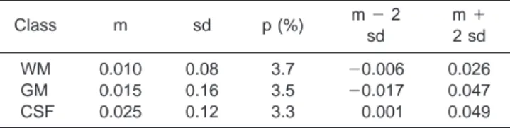
was plotted against their mean value. The mean of the differences m and their standard deviation sd were then computed. Table 4 shows the results for WM, GM, and CSF.

The WCC membership may be -0.006 below or 0.026 above the membership value given by the clustering of the (T1-, T2-, and proton density-weighted) value for the white matter. Likewise, the membership computed by WCC for the GM can be -0.017 below or 0.047 above that computed with the MR-weighted images, and -0.001 below or 0.049 above for the CSF. WCC tended

to give a higher membership, but the limits of agree-ment were small enough for us to be confident that the two methods agreed when clustering the same brain. WCC thus provided reliable results for brain tissue seg-mentation. What makes it interesting is that clustering was done on one image only, with statistically the same results as with multidimensional validated clustering. This was a great advantage, considering that registra-tion of multimodal images is an acute problem.

Concerning the acquisitions, the MR data set con-sisted of data with poor resolution (128 ⫻ 128 ⫻ 64, Figure 6. Fuzzy tissue maps generated by multidimensional signal analysis and WCC.

with 2⫻ 2 ⫻ 2 mm3_{voxels). This made the}

segmenta-tion problem more difficult because of increased partial volume effects. Nevertheless, PCA applied with the wavelet coefficients vectors to a single acquisition suc-ceeded in segmenting GM, WM, and CSF at least as well as a multispectral analysis according to our statistical test.

Comparison With Other Methods of Segmentation

Lastly, the clustering obtained with PCA and the wave-let coefficients vectors was compared with other meth-ods of segmentation. No algorithm has emerged in the literature as clearly superior because segmentation of MR data is intrinsically limited (partial volume effect, noise) (42). Moreover, the absence of a gold standard makes it difficult to assess the results of a segmentation process precisely. In this section, our clustering algo-rithm is compared with several others algoalgo-rithms, in terms of labeled images. The methods were chosen so that a wide range of algorithms was covered (monospec-tral, multispec(monospec-tral, parametric, nonparametric). The brain used for the estimation of the parameter m was once more clustered. It was acquired in two sets of images: T1-, T2-, and proton density-weighted regis-tered images (Set 1) on the one hand, and a FLASH 3D sequence (Set 2) on the other hand. Several methods were applied to process a labeled brain:

1. A multispectral histogram analysis (16) (MHA) and a multispectral maximum likelihood expectation (MMLE) on Set 1.

2. A monospectral maximum likelihood expectation (MLE), the k-nearest neighbors algorithm (KNN), and PCA with the wavelet coefficients vectors on Set 2.

The reference volume, labeled by a trained specialist, was also available.

Table 5 presents the Tanimoto coefficients (35) of the methods with respect to the labeled reference image. The best results were obtained with the multispectral histogram analysis. Relevant information were avail-able in this method, leading to a mean Tanimoto index of 0.76 for the three classes of tissues. MMLE gave lower results, due to the statistical assumption of the algorithm. Concerning methods performed on a single acquisition, PCA gave the best results, approaching those of MHA except for GM. Agreement between the labeled reference image and the one computed by our algorithm ranged from 0.71 for GM to 0.78 for WM. This meant that the two labeled images agreed at least 3 times more than they disagreed. MLE produced the

worst results (because of the statistical assumption and the unique acquisition provided to the algorithm) while KNN gave lower Tanimoto coefficients than our method did for GM and CSF, and an equal index for WM, indi-cating a worse clustering.

Thus our method gave roughly the same results as the multispectral histogram analysis. However, it offers the great advantage of requiring only one MR volume.

CONCLUSIONS

Of the various MR segmentation processes proposed in the literature, none separates tissues reliably enough to be used without the interpretation of a radiologist. We propose a method designed to assist the physician by assigning fuzzy memberships to voxels, representing the possibility they have of belonging to cerebral tis-sues. Crisp images can be obtained to quantify and measure brain volumes.

The method never failed to produce a set of fuzzy tissue maps. We have shown that the possibilistic clus-tering algorithm on the wavelet coefficients vectors will reliably discriminate the different brain compartments (WM, GM, and CSF), first by comparing its results with those provided by a fuzzy model of brain tissues, and second by assessing its performance against other fea-ture vectors and methods. The frame of fuzzy logic al-lows for ambiguity and uncertainty in MR images (par-tial volume averaging, noise) by assigning a voxel to all brain tissues with different absolute memberships. Wavelet coefficients extract relevant information in the image, from structural to textural, thus improving the quality of voxel properties to be clustered. The ability to apply the whole process to a single MR image also offers an advantage over most segmentation methods that require multispectral and registered images.

Further improvements in our classification process include integration of the radiofrequency inhomogene-ity correction. Although it raises minimal problems when making qualitative assessments on the images, this inhomogeneity introduces a spatial modulation in signal levels across the image and impedes accurate quantification of brain tissue volumes, as shown in the discussion. Another improvement is the introduction of another kind of information before the final segmenta-tion, for example, by means of fuzzy rules or simplified atlas localization. The main objective here is to reduce Table 4

Bland and Altman Analysis of the Two Clustering Methods*

Class m sd p (%) m⫺2 sd m⫹ 2 sd WM 0.010 0.08 3.7 _⫺0.006 0.026 GM 0.015 0.16 3.5 _⫺0.017 0.047 CSF 0.025 0.12 3.3 0.001 0.049

*m⫽mean, sd⫽standard deviation, p⫽percentage of difference outside the interval [m⫺2䡠sd, m⫹2䡠sd].

Table 5

Tanimoto Coefficients of Several Methods With Respect to a Referenced Labeled Image*

Set of images (method)

Tissue Set 1 Set 2

MHA MMLE MLE KNN PCA

CSF 0.75 0.73 0.64 0.70 0.73

GM 0.76 0.70 0.57 0.67 0.71

WM 0.78 0.73 0.68 0.78 0.78

*MMLE ⫽ multispectral maximum likelihood expectation, MHA⫽ multispectral histogram analysis, MLE ⫽ monospectral maximum likelihood expectation, KNN ⫽ the k-nearest neighbors algorithm (KNN), PCA ⫽ possibilistic clustering algorithm with the wavelet coefficient vectors.

the effect of partial volume averaging on the boundaries of the ventricles. All these improvements are expected to benefit the final segmentation.

ACKNOWLEDGMENTS

The authors thank Jean Marie Bonny (INRA, France), Prof. Jean-Jacques Lemaire (ERIM, Faculty of Medi-cine, Clermont Ferrand, France), and Arnaud Colin (MDS, Miami, FL) for their constructive suggestions and many helpful comments, as well as Mr. John Ryan (ATT, France) for help with the English.

APPENDIX: THE FUZZY CLUSTERING PROBLEM

The main idea behind fuzzy clustering is that an object can belong simultaneously to more than one class and does so to varying degrees called memberships. The use of fuzzy logic in image processing offers two advantages: the possibility of overcoming the crisp nature of pattern descriptions, as they can be used for algorithms, and the inclusion of human intentions in the process. Two algorithms are often used in the field of fuzzy clustering: the fuzzy C-means algorithm introduced by Bezdek (10), or one of its derivatives, such as the possibilistic clustering algorithm (28).

The Fuzzy C-Means Algorithm

The fuzzy C-means algorithm is an iterative method, which searches for compact clusters. It associates with every p-dimensional feature vector X⫽ (xj, j ⫽ 1. . .N,

xj僆 R

p_{) a fuzzy membership grade u}

i,j僆 [0,1] in each of

the C classes 1ⱕ j ⱕ C, representing the degree that xi

has to belong to j. It uses iterative optimization to ap-proximate minima of a constrained objective function:

J共B, U, X兲 ⫽

冘

冘

where biis the center of cluster i, m⬎ 1 is a parameter

controlling the degree of fuzzification, and d is a dis-tance.

Krishnapuram and Keller (28) showed that this algo-rithm creates relative memberships, interpreted as de-grees of sharing of the voxels between all the classes, that are thus unrepresentative of the true degree of belonging. Fuzzy C-means actually produces an ana-lytic formulation of uijthat depends on the distances of

xjto all class centers bkand not only on d(xj,bi). They

thus proposed a new version, called the possibilistic clustering algorithm that allows uijto depend only on

d(xj,bi).

The Possibilistic Clustering Algorithm

PCA consists of minimizing a new objective function under new constraints. The aim is to minimize

J共B, U, X兲 ⫽

冘

冘

冘

冘

where niis a positive number that determines the

dis-tance at which the membership value of a feature in the cluster i becomes 0.5.

Krishnapuram and Keller (28) proved that this algo-rithm allows the memberships to be interpreted in terms of absolute memberships of features to clusters. In other words, the PCA membership of a vector xj to

class i only depends on xjand i, and not on the

mem-berships of xjin all other classes (as is the case for fuzzy

C-means). This is very convenient in the case of strong ambiguity or uncertainty, which can occur in MR im-ages (partial volume effect, noise), as shown by clear examples in Krishnapuram and Keller (28).

REFERENCES

1. Bezdek JC, Hall LO, Clarke LP. Review of MR image segmentation techniques using pattern recognition. Med Phys 1993;20:1033– 1048.

2. Choi H, Haynor D, Kim Y. Partial volume tissue classification of multichannel MR images—a mixed model. IEEE Trans Med Imag-ing 1991;10:395– 400.

3. Ashton EA, Berg MJ, Parker KJ, et al. Segmentation and feature extraction techniques with applications to MRI head studies. Magn Reson Med 1995;33:670 – 677.

4. Jaggi C, Ruan S, Fadili J, Bloyet D. A markovian approach for 3D segmentation of cerebral tissues in MRI. Colloque GRETSI 1997; 16:327–330.

5. Vinitski S, Gonzales C, Burnett C, et al. Tissue segmentation by high resolution MRI: improved accuracy and stability. In: Proceed-ings of the IEEE Engineering in Medicine and Biology Society 16th Annual International Conference, Baltimore, MD, 1994. p 557–558. 6. Raff U, Scherzinger A, Vargas P, Simon J. Quantitation of gray matter, white matter and cerebrospinal fluid from spin-echo mag-netic resonance images using an artificial neural network tech-nique. Med Phys 1994; 12:1933–1942.

7. Herndon RC, Lancaster JL, Toga AW, Fox PT. Quantification of white matter and gray matter volumes from T1 parametric images using fuzzy classifiers. J Magn Reson Imaging 1996;6:425– 443. 8. Clarke LP, Velthuizen RP, Phuphanich S, et al. MRI: stability of

three supervised segmentation techniques. Magn Reson Imaging 1993;11:95–106.

9. Philipps WE, Velthuizen RP, Phuphanich S, et al. Application of fuzzy C-means algorithm segmentation technique for tissue differ-entiation in MR images of a hemorrhagic glioblastoma multiforme. Magn Reson Imaging 1995;13:277–290.

10. Bezdek JC. Pattern recognition with fuzzy objective function algo-rithms. New York: Plenum Press, 1981.

11. Bezdek JC, Hall LO, Clark M, Goldof D, Clarke LP. Medical image analysis with fuzzy models. Stat Methods Med Res 1997;6:191– 214.

12. Brandt ME, Bohan TP, Kramer LA, Fletcher JM. Estimation of CSF, white and gray matter volumes in hydrocephalic children using fuzzy clustering of MR images. Comput Med Imaging Graphics 1994;18:25–34.

13. Clark M, Hall LO, Goldgof DB, et al. MRI segmentation using fuzzy clustering techniques. In: Proceedings of the IEEE Engineering in Medicine and Biology Society 16th Annual International Confer-ence, Baltimore, MD, 1994. p 730 –742.

14. Deaton R, Tang L, Reddick WE. Fractal analysis of MR images of the brain. In: Proceedings of the IEEE Engineering in Medicine and Biology Society 16th Annual International Conference, Baltimore, MD, 1994. p 260 –262.

15. Agartz I, Sa¨a¨f J, Wahlund LO, Wetterberg L. Quantitative estima-tions of cerebrospinal fluid spaces and brain regions in healthy controls using computer-assisted tissue classification of MR im-ages: relation to age and sex. Magn Reson Imaging 1992;10:17– 226.

16. Fletcher LM, Barsotti JB, Hornak JP. A multispectral analysis of brain tissues. Magn Reson Med 1993;29:623– 630.

17. Gasperini C, Horsfield M, Thorpe J, et al. Macroscopic and micro-scopic assessments of disease burden by MRI in multiple sclerosis: relationship to clinical parameters. J Magn Reson Imaging 1996; 6:580 –584.

18. Kiviniitty K. NMR relaxation times in NMR imaging. Ann Clin Res 1984;16:4 – 6.

19. Just M, Thelen M. Tissue characterization with T1, T2 and proton density values: results in 160 patients with brain tumors. Radiol-ogy 1988;169:779 –785.

20. Lim K, Pfefferbaum A. Segmentation of MR brain images into cere-brospinal fluid spaces, white and gray matter. J Comput Assist Tomogr 1989;13:588 –593.

21. Reiss A, Hennessey JG, Rubin M, et al. Reliability and validity of an algorithm for fuzzy tissue segmentation. J Comput Assist Tomogr 1998;12:1933–1942.

22. Barra V, Colin A, Boire JY. Synthesis of a high resolution functional image by MR/SPECT fusion process. Eur J Nucl Med 1998;5:490. 23. Haase A, Frahm J, Matthaei D, Ha¨nicke W, Merboldt K-D. FLASH imaging. Rapid NMR imaging using low flip-angle pulses. J Magn Reson 1986;67:258 –266.

24. Pelc N. Optimization of flip angle for T1 dependent contrast in MRI. Magn Reson Med 1993;29:695– 699.

25. Di Gesu V, Romeo L. An application of integrated clustering to mri segmentation. Pattern Recognition Lett 1994;15:731–738. 26. Zadeh L. Fuzzy sets. Information Control 1965;8:338 –353. 27. De la Paz R, Bernstein R, Hanson W, Walker M. Approximate fuzzy

C-means cluster analysis of medical MR images data. A system for medical research and education. IEEE Trans Geosci Remote Sens-ing 1986;25:815– 824.

28. Krishnapuram R, Keller JM. A possibilistic approach to clustering. IEEE Trans Fuzzy Systems 1993;1:98 –110.

29. Tucker W. Counterexamples to the convergence for the fuzzy iso-data algorithms. In: The analysis of fuzzy information. Boca Raton, CRC Press, FL; 1987.

30. Gath I, Geva B. Unsupervised optimal fuzzy clustering. IEEE Trans PAMI 1989;11:773–781.

31. Dave RN. Fuzzy shell clustering and application to circle detection in image processing. Int J Gen Systems 1990;41:343–355.

32. Barra V, Boire JY. Cerebral tissues characterization in MR images by possibilistic clustering on voxel feature vectors, In: Proceedings of 6e`mes Rencontres de la Socie´te´ Francophone de Classification, Montpellier, France, 1998. p 15–19.

33. Daubechies I. Orthonormal bases for compactly supported wave-lets. Commun Pure Appl Math 1988;16:909 –966.

34. Kwan R, Evans A, Pike B. An extensible MRI Simulator for post-processing evaluation. In: Visualization in biomedical computing, lecture notes in computer sciences. New York: Springer-Verlag; 1996. p 1131:135–140.

35. Duda RO, Hart PE. Pattern classification and scene analysis. New York: Wiley; 1973.

36. Shaltenbrand G, Bailey P. Introduction to stereotaxis with an atlas of the human brain, vol. II. Stuttgart: George Thieme Ver-lag, 1959.

37. Matsumae M, Kikinis R, Mo´rocz I, et al. Age-related changes in intracranial compartment volumes in normal adults assessed by magnetic resonance imaging. J Neurosurg 1996;84:982–999. 38. Miller AK, Alston RL, Corsellis JA. Variation with age in the

vol-umes of gray and white matter in the cerebral hemispheres of man: measurements with an image analyser. Neuropathol Appl Neuro-biol 1980;6:119 –132.

39. De la Monte SM. Quantification of cerebral atrophy in pre-clinical and end-stage Alzheimer’s disease. Ann Neurol 1989;25:450 – 459. 40. Bensaid AM, Hall LO, Bezdek JC, Clarke LP. Fuzzy cluster validity in magnetic resonance images. In: Proceedings of the SPIE Confer-ence on Medical Imaging, 1994. p 454 – 464.

41. Bland JM, Altman DG. Statistical methods for assessing agreement between two methods of clinical measurement. Lancet 1986;8:307– 310.

42. Links JM, Beach LS, Subramaniam B, et al. Edge complexity and partial volume effects. J Comput Assist Tomogr 1998;22:450 – 458.