A bi-criteria evolutionary algorithm for a constrained multi-depot vehicle routing problem
Texte intégral
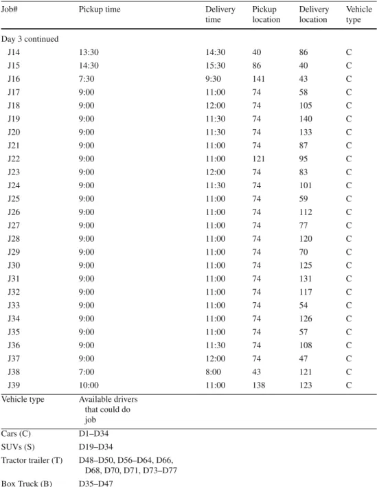
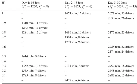
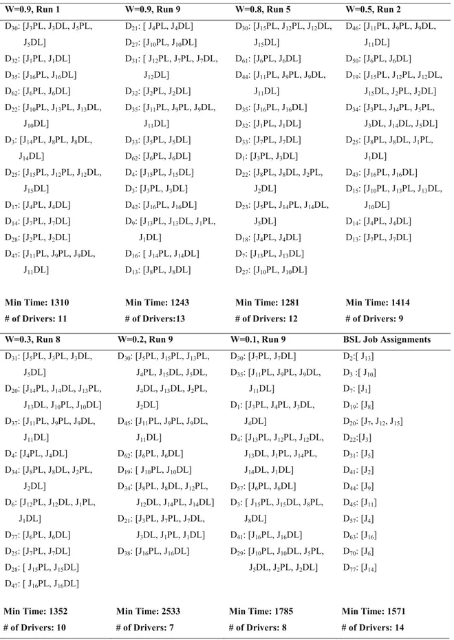
Figure


Documents relatifs
To sum up, the main contributions of this article are: 1) A new meta-heuristic that is highly effective for three important vehicle routing problem classes, the MDVRP, the PVRP, and
The common scheme on which all the heuristics are based consists in, after having found an initial solution, applying a local search phase, followed by a diversification; if the
Periodic Vehicle Routing Problem (PVRP), time windows, hybrid genetic algorithm, meta-heuristics, tabu search, variable neighborhood search.. Partial funding for this project has
Routes are constructed by solv- ing a vehicle routing problem for each day using Clarke and Wright savings algorithm (Clarke and Wright [1964]). Then, for the shaking phase two
Using our model and algorithm we are able to evaluate the impact of each parameter of the problem, namely the number of customers, products, vehicles and periods, in terms
We approximate the production fluctuations over the horizon T using a sequence of periods (day clusters), with the same produc- tion level within each period, forming a
The proposed multi-period model has some similarities to an a priori optimization framework in the context of the vehicle routing problem with stochastic demand (VRPSD). In a
The proposed multi-period model has some similarities to an a priori optimization framework in the context of the vehicle routing problem with stochastic demand (VRPSD). In a
