A probabilistic model for data cube compression and query approximation

(1)

Publisher’s version / Version de l'éditeur:

Vous avez des questions? Nous pouvons vous aider. Pour communiquer directement avec un auteur, consultez la première page de la revue dans laquelle son article a été publié afin de trouver ses coordonnées. Si vous n’arrivez pas à les repérer, communiquez avec nous à PublicationsArchive-ArchivesPublications@nrc-cnrc.gc.ca.

Questions? Contact the NRC Publications Archive team at

PublicationsArchive-ArchivesPublications@nrc-cnrc.gc.ca. If you wish to email the authors directly, please see the first page of the publication for their contact information.

https://publications-cnrc.canada.ca/fra/droits

L’accès à ce site Web et l’utilisation de son contenu sont assujettis aux conditions présentées dans le site LISEZ CES CONDITIONS ATTENTIVEMENT AVANT D’UTILISER CE SITE WEB.

The ACM Tenth International Workshop on Data Warehousing and OLAP

[Proceedings], 2007

READ THESE TERMS AND CONDITIONS CAREFULLY BEFORE USING THIS WEBSITE.

https://nrc-publications.canada.ca/eng/copyright

NRC Publications Archive Record / Notice des Archives des publications du CNRC :

https://nrc-publications.canada.ca/eng/view/object/?id=aede0cb1-b744-4692-a39b-af0315612a67

https://publications-cnrc.canada.ca/fra/voir/objet/?id=aede0cb1-b744-4692-a39b-af0315612a67

NRC Publications Archive

Archives des publications du CNRC

This publication could be one of several versions: author’s original, accepted manuscript or the publisher’s version. / La version de cette publication peut être l’une des suivantes : la version prépublication de l’auteur, la version acceptée du manuscrit ou la version de l’éditeur.

Access and use of this website and the material on it are subject to the Terms and Conditions set forth at

A probabilistic model for data cube compression and query

approximation

(2)

National Research Council Canada Institute for Information Technology Conseil national de recherches Canada Institut de technologie de l'information

A Probabilistic Model for Data Cube

Compression and Query Approximation *

Missaoui, R., Goutte, C., Kouomou Choupo, A., Boujenoui, A.

November 2007

* published at The ACM Tenth International Workshop on Data

Warehousing and OLAP. Lisbon, Portugal. November 9, 2007. NRC

49870.

National Research Council of Canada

Permission is granted to quote short excerpts and to reproduce figures and tables from this report, provided that the source of such material is fully acknowledged.

(3)

A Probabilistic Model for Data Cube Compression and

Query Approximation

Rokia Missaoui

University of Quebec in Outaouais P.O. Box 1250, Suc. B Gatineau, Quebec, J8X 3X7, Canada

rokia.missaoui@uqo.ca

Cyril Goutte

Interactive Language Technology NRC Institute for Information Technology

283, Alexandre-Taché Gatineau, QC J8X 3X7, Canada

Cyril.Goutte@nrc-cnrc.gc.ca

Anicet Kouomou Choupo

University of Quebec in Outaouais P.O. Box 1250, Suc. B Gatineau, Quebec, J8X 3X7, Canada

akchoupo@yahoo.fr

Ameur Boujenoui

School of Management, University of Ottawa 136 Jean-Jacques Lussier

Ottawa, ON, K1N 6N5, Canada

boujenoui@management.uottawa.ca

ABSTRACT

Databases and data warehouses contain an overwhelming volume of information that users must wade through in or-der to extract valuable and actionable knowledge to support the decision-making process. This contribution addresses the problem of automatically analyzing large multidimen-sional tables to get a concise representation of data, identify patterns and provide approximate answers to queries.

Since data cubes are nothing but multi-way tables, we propose to analyze the potential of a probabilistic model-ing technique, called non-negative multi-way array factor-ization, for approximating aggregate and multidimensional values. Using such a technique, we compute the set of com-ponents (clusters) that best fit the initial data set and whose superposition approximates the original data. The gener-ated components can then be exploited for approximately answering OLAP queries such as roll-up, slice and dice oper-ations. The proposed modeling technique will then be com-pared against the log-linear modeling technique which has already been used in the literature for compression and out-lier detection in data cubes. Finally, three data sets will be used to discuss the potential benefits of non-negative multi-way array factorization.

Categories and Subject Descriptors

H.2.8 [Information Systems]: Database Applications—

data mining; H.4.2 [Information Systems]: Types of

Sys-tems—decision support

Permission to make digital or hard copies of all or part of this work for personal or classroom use is granted without fee provided that copies are not made or distributed for profit or commercial advantage and that copies bear this notice and the full citation on the first page. To copy otherwise, to republish, to post on servers or to redistribute to lists, requires prior specific permission and/or a fee.

General Terms

Algorithms, experimentation

1. INTRODUCTION

In many database and data warehouse applications, users tend to (1) be drowned in data and even in knowledge dis-covered from data, (2) use more dimensions (variables) than necessary to explain a set of phenomena and check prede-fined hypotheses, and (3) analyze a generally heterogeneous population of observations/individuals. In order to reduce their memory overload and working space induced by their tendency for over-dimensioning and the inherent heterogene-ity and huge volume of data, we propose to use a probabilis-tic modeling technique, called non-negative multi-way array factorization (NMF), to identify patterns and approximate data and query answers. Such a technique will then be com-pared to log-linear modeling (LLM).

Many topics have attracted researchers in the area of data warehousing: data warehouse design and multidimen-sional modeling, materialized view selection, efficient cube computation, query optimization, discovery-driven explo-ration of cubes, cube reorganization, cube mining, and so on. Recently, there has been an increasing interest for ap-plying/adapting data mining techniques and advanced sta-tistical analysis (e.g., cluster analysis, principal component analysis, log-linear modeling) for knowledge discovery [21, 19, 24, 18] and data compression in data cubes [3, 4, 5, 13]. In [24], an approach based on log-linear modeling is used to identify exceptions in data cubes by comparing antici-pated cell values against actual values. In [4, 5], log-linear modeling is used for data compression.

Approximate query answering in data warehouses has been used in order to accelerate aggregate computation and query execution at the expense of some information loss. Existing work has been conducted based mainly on sampling [3, 13], clustering [29], wavelets [7] or maximum entropy prin-ciple [23]. Palpanas et al. [23] propose an approach based on information entropy to (i) detect deviations, and (ii) es-timate the original multidimensional data from aggregates for approximate query answering purposes. A wavelet-based

(4)

approach is used in [7] to approximate query answering, and proves to be more effective than sampling techniques. In a similar spirit, [26] uses the probability density distribution of data in order to propose a compressed representation of data cubes which reduces data storage and leads to approximate answers to aggregate queries. Wavelet based techniques have been used either for progressive evaluation of some specific OLAP queries [2, 7] or as a sampling technique. As in [26], Vitter et al. [27] use wavelets for compressing sparse data cubes and getting approximate answers of aggregate queries. In [22], an approach towards the approximation of the an-swer to OLAP queries and the identification of classification and characteristic rules is proposed using the rough set the-ory. It allows the user to get an approximate answer to his query either in a restricted mode using a cube lower approximation or in a relaxed mode using cube upper ap-proximation.

The NMF approach was initially developed for analyzing two-dimensional data [20], and generalizes easily to higher dimensional data [28]. It has been applied to analyze vari-ous data such as image, music, text or medical signals (see Section 6 of [15] for further references). To the best of our knowledge, NMF has never been applied to the analysis and exploration of data cubes.

The paper is organized as follows. First, we describe a real-life running example in Section 2 and provide in Sec-tion 3 some background about probabilistic modeling using NMF or LLM. Section 4 aims to show the potential of the se-lected modeling technique for cube approximation, compres-sion and OLAP querying. Section 5 provides a discuscompres-sion of the two modeling techniques while Section 6 summarizes our findings and future work.

2. AN ILLUSTRATIVE EXAMPLE

We now introduce the running example that will be used in the sequel to illustrate the use of NMF for cube modeling and approximation. It is based on a study conducted on a sample of 214 Canadian firms listed on the Stock Market and aimed at establishing links between corporate gover-nance practices and other variables such as the shareholding structure [6, 15]. Governance is defined as the means, prac-tices and mechanisms put in place by organizations to ensure that managers are acting in shareholders’ interests. Gover-nance practices include, but are not limited to, the size and the composition of the Board of Directors, the number of in-dependent directors and women sitting on the Board as well as the duality between the position of CEO and the position of Chairman of the Board. Based on the collected data, a data warehouse has been constructed with sixteen dimen-sions and an initial set of fact tables for data cube mining and exploration. Table 1 is a fact table which provides the number of firms according to four dimensions: USSX, Du-ality, Size, and QI. USSX∈ {Yes, No} indicates whether the firm is listed or not on a US Stock Exchange. Du-ality ∈ {Yes, No} indicates whether the CEO is also the Chairman of the Board. Size ∈ {1, 2, 3, 4} represents the size of the firms in terms of the log of their assets. The values are 1 (< 2), 2 (≥ 2 and < 3), 3 (≥ 3 and < 4) and 4 (≥ 4). QI expresses the index of corporate governance quality and takes one of the following values (from worst to best quality): Low (< 40%), Medium (≥ 40 and < 70%), and High (≥ 70%).

Duality: No Yes USSX Size QI:Low Med High Low Med High

1 0 7 0 4 3 0 No 2 7 21 12 6 12 4 3 11 13 11 4 4 2 4 0 3 1 0 2 0 1 0 1 2 0 0 0 Yes 2 4 12 0 7 10 1 3 4 4 14 5 8 2 4 0 3 7 0 2 1

Table 1: Data cube for the Governance example.

3. PROBABILISTIC DATA CUBE MODELS

Consider a n-dimensional data cube X, and assume that the measure in each cell is a frequency xi₁i₂...in∈ N.

1 With-out loss of generality and to simplify notation, we will use n = 3 from now on. The three dimensions are denoted A, B and C, with respective modalities {ai}i=1...I, {bj}j=1...J, and {ck}k=1...K. Each cell xijk of the 3-dimensional cube X = [xijk] therefore contains the count of the number of observations of the three modalities (ai, bj, ck).

Information contained in a high dimensional data cube may be difficult to access or visualize. For example, it may be hard to identify which dimensions interact, or which parts of the cube display consistent patterns. Probabilistic mod-els such as NMF and log-linear modmod-els can discover such in-teractions and patterns, by finding a concise representation that provides a faithful approximation of the data. The use of a concise model reduces both storage space and processing time, while a good approximation ensures that queries per-formed on the model return reasonably accurate answers. A probabilistic model assigns a probability P (i, j, k) to the ob-servation of the tuple of modalities (ai, bj, ck). The fit of the model to the observations is measured by the log-likelihood:

L = − log P (X|θ) = −X ijk

xijklog P (i, j, k), (1) The most flexible, or saturated, model estimates each P (i, j, k) based on the data, i.e., bP (i, j, k) = xijk/N , with N = P

ijkxijk. This model essentially reproduces the data with-out modeling any interesting or systematic effect. In our ex-ample, this means that it is not possible to discover that the quality of the governance QI is strongly dependent on the duality. On the other hand, the independence model assumes that all variables are independent: bP (i, j, k) = bP (i) bP (j) bP (k), with Maximum Likelihood estimates: bP (i) = Pjkxijk/N , (and similarly for j and k). This model is parsimonious (i.e., has a small number of parameters) but too simple (and of-ten unrealistic) since it does not model interactions between variables. In our example, it means that the independence model will ignore the strong interaction between QI and Du-ality, i.e., it yields similar probability for high governance quality, regardless of the value of Duality.

Useful models usually fall somewhere in between these two extremes: they strike a balance between expressive power (good approximation) and parsimony (few parameters).

1_{This assumption can be easily relaxed to take into account} values other than frequencies.

(5)

3.1 Non-negative Multi-way Array

Factorization

The model associated with NMF is a mixture of condi-tionally independent multinomial distributions. It general-izes Probabilistic Latent Semantic Analysis [17], commonly used for text applications, to more than two dimensions:

P (i, j, k) = M X m=1 P (m)P (i|m)P (j|m)P (k|m) (2) = M X m=1 Wm⊗Hm⊗Am,

where m is a given component and M the number of com-ponents. The latter controls the flexibility of the model. More components allow more free parameters and a better approximation of the data, but too much flexibility yields over-training, i.e., a model that over-represents artifacts of the data at the expense of the underlying phenomenon. The parameters Wm_{, H}m _{and A}m _{are the m-th columns of} the I × M matrix W = [P (m)P (i|m)], the J × M matrix H = [P (j|m)] and K × M matrix A = [P (k|m)] respec-tively. As P (i, j, k) ≈ _N1X, matrices W, H and A are a fac-torization of cube X. Since they contain probabilities, the factors are also non-negative. The mixture model in Equa-tion 2 is therefore an instance of Non-negative Multi-way

array Factorization [28], a generalization of Non-negative

Matrix Factorization [20]. Parameters are estimated by

Maximum Likelihood, which is conveniently done using the Expectation-Maximization (EM, [11]) algorithm. Several al-ternative algorithms exist for NMF in 2D [12], but algo-rithms currently proposed for n > 2 minimize either the Kullback-Leibler divergence (equivalent to Maximum Like-lihood, see [14]) or squared error [28]. The parameter esti-mation procedure is as follows:

• Initialize mixture weights P (m) and profiles P (i|m), P (j|m), etc. to uniform distributions plus small ran-dom perturbation. • Iterate over t = 0 . . . : Pt+1(m) ← Pt_(m)X ijk “x_ijk N ”Pt(i|m)Pt(j|m)Pt(k|m) Pt_{(i, j, k)} Pt+1(i|m) ← P t_(i|m)Pt_(m) Pt+1_(m) X jk “x_ijk N ”Pt(j|m)Pt(k|m) Pt_{(i, j, k)} and similarly for P(t+1)(j|m) and P(t+1)(k|m) [15]. • until the increase in likelihood is smaller than a small

threshold (e.g., 10−6_).

The main modeling issue is therefore to select the correct number of components. Although the NMF literature of-ten ignores this issue, the probabilistic modeling framework offers tools for selecting the appropriate model complexity. One solution is to rely on information criteria such as AIC [1] or BIC [25]. Defining the (log) likelihood ratio as twice the difference in log-likelihood between the fitted model and the saturated model, G2 _{= 2}P

ijkxijklogb

x_ijk

xijk, and df the

num-ber of degrees of freedom, i.e., the difference in the numnum-ber of free parameters between the fitted model and the satu-rated model, df = IJK − (I + J + K − 2) × M , we have:

AIC = G2− 2df and BIC = G2− df × log N (3)

The number M of components with the lowest AIC (or BIC) is then selected.

As components are represented by profiles along the var-ious dimensions, P (i|m), P (j|m) and P (k|m), each com-ponent may select a subset of modalities, by setting other probabilities to zero. One key feature of NMF is its ability to identify dense sub-cubes (expressed by components) inside the original, possibly sparse, data cube. Such a feature can then be exploited to approximate query answers using ap-propriate components (see Subsection 4.3) or to conduct fur-ther analysis on components using, for example, log-linear modeling.

3.2 Log-Linear Modeling

As indicated earlier, log-linear modeling has been used in the field of data warehousing for data approximation and outlier detection. The principle of this modeling technique [9] is to decompose the log-probability of given cell value as an additive sum of terms involving all combinations of subsets of dimensions: log P (i, j, k) = λ + λAi + λ B j + λ C k+ λ AB ij + λ AC ik + λ BC jk + λ ABC ijk (4) where λ is the overall mean (in the log domain) and all other parameters model the effect of a subset of the dimensions, e.g. λBC

jk models the joint effect of observing B = bjand C = ck, regardless of variable A. In order to have an identifiable model, the marginals of the parameters are constrained to zero: P_iλA i = P jλ B j = P kλ C k = 0, P iλ AB ij = P jλ AB ij = 0, etc.

When all terms are present in Equation 4, this corresponds to the saturated model. The complexity of the model may be controlled by removing some parameters (or setting them to zero), which adds the corresponding degrees of freedom. Of course, as parameters are removed, the model deviates pro-gressively from data. Therefore, selecting the appropriate model is again a compromise between parsimony and ap-proximation. This may conveniently be done using iterative model selection methods such as forward selection or back-ward elimination. In backback-ward elimination, one starts with a large model, for example the saturated model, and itera-tively eliminates interactions (from higher to lower order), as long as the associated increase in G2 _{is not significant} at a pspecified level (usually 95%), until none of the re-maining interactions may be eliminated. Forward selection proceeds the opposite way by starting with a small model (generally the independence model) and then adding inter-actions of increasing order. The parameters of the model may be obtained either by directly optimizing the likeli-hood with a Newton-Raphson algorithm [16], or by using the Iterative Proportional Fitting (IPF) procedure [10], a dedicated method for modeling multi-way frequency tables. These techniques may also be used together with informa-tion theoretic criteria such as the AIC or BIC (see Equainforma-tion 3). Note that in the context of LLM, AIC seems to be pre-ferred [9].

The most popular log-linear models are hierarchical mod-els: all lower-order effects within higher-order ones are nec-essarily included. A common notation for hierarchical log-linear models is therefore to specify only terms with the highest order interaction. For example, {A ∗ B, A ∗ C} de-notes the hierarchical model containing A ∗ B and A ∗ C as well as first order terms A, B and C.

(6)

3.3 Rates of compression and approximation

The goal of probabilistic modeling is to produce an ap-proximation of the data cube that uses as few parameters as possible. We will therefore be interested in measuring the compression rate and the approximation quality for each model. The compression rate is linked to the ratio of the number of free parameters f in the model and the total number of cells in the cube, Nc, and is defined as:

Rc= 1 − f Nc = df Nc (5) With df the number of degrees of freedom defined above. By definition, the saturated model has a compression rate of 0% since f = Nc.

Typical probabilistic models offer a direct way to control the compression rate by tuning the model complexity. For NMF, the compression decreases linearly as the number of components grows. In our three dimensional example, Nc= I ×J ×K and, with M components, f = (I +J +K −2)∗M , such that:

RN M Fc = 1 − M

I + J + K − 2

IJK (6)

In the situation where the components are sparse, i.e., many parameters are zero,2an arguably better way to mea-sure the compression offered by the model is to take into account the non-zero parameters only. In such a situation, Equations 5 and 6 are lower bounds that offer a minimum guaranteed compression rate for a model with the given number of components.

The approximation quality may be measured in various ways such as the mean squared error or the mean absolute error. In the context of probabilistic models, it is measured by the log-likelihood (Equation 1) or, equivalently, the de-viance G2. The deviance offers a “standard” way to measure the approximation quality: perfect approximation yields a deviance of 0 and higher deviance means worse approxima-tion, so it is a good way to compare various models of the same data cube. However, there is to our knowledge no way to offer a guaranteed approximation level a priori for a given data cube and model complexity (i.e., number of components in NMF or number of interactions in LLM). The optimal approximation error depends on the level of noise in the data. In typical situations, the noise level is unknown before modeling, therefore the resulting approxi-mation level can not be guaranteed. Note however that for most probabilistic models, increasing the model complexity will systematically improve the approximation of the data on which the model is estimated. If a given approximation level is required, it is straightforward to increase the model complexity, e.g., by adding components in NMF, until the minimum deviance is reached.

4. DATA COMPRESSION, APPROXIMATION,

AND RETRIEVAL

Besides the Governance data cube described in Sec-tion 2, we used two synthetic data sets to illustrate the po-tential of NMF for data approximation/compression as well as approximate query answering. One of the sets is a simpli-fied version of a dimension table called Customer of Food 2_{Near-zero parameters may usually be pruned from the} model with no loss in approximation.

Cubes

Features Governance Customer Sales Nb. of dimensions 4 5 3 Nb. of cells 48 2400 528 Nb. of records 214 10281 5191 Highest nb. modalities 4 8 44 Density 63% 37% 50%

Table 2: Features of the three data cubes. “Density” is the ratio of non-zero cells.

mart data delivered with Analysis Services of Microsoft SQL Server. From the Customer table (10281 records) we constructed a data cube of five dimensions: Status, Income, Child, Occupation and Education. Status ∈ {1, 2} indicates whether the customer is single (value equal to 1) or not. Income takes eight possible values indicating the level of income (e.g., 1 for income between 10K and 30K, and 8 for income ≥ 150K). Child ∈ {0, 1, 2, 3, 4, 5} repre-sents the number of children. Occupation takes five possi-ble values indicating the customer’s occupation (e.g., 1 for a manual worker and 5 for a manager). Education refers to customer’s education level and can take five possible values (e.g., 1 for partial high school studies and 5 for graduate studies). The other data set was also extracted from Food martdata and concerns a data cube of Sales according to product category (44 values), time (in quarters) and coun-try (USA, Canada and Mexico). This cube has a relatively small set of dimensions but one of them has a large number of modalities (members).

Table 2 summarizes the features of the three data cubes in terms of their dimensionality, the number of members per dimension, the number of records/instances, the number of cube cells as well as the density. The first cube was selected because it represents real data while the other ones were retained for their relatively higher size or dimensionality.

4.1 Model Estimation

We illustrate model estimation for both NMF and LLM through the Governance cube.

For NMF, the information criterion AIC identifies three components (see Figure 1). Therefore, the user can see these components as a way to cluster the initial cube into ho-mogeneous data sets, and hence can focus his analysis on some identified components rather than the whole popula-tion (cube). The first component C1 represents only 16% (P (C1) = 0.16) of the observations and corresponds to com-panies with no duality (i.e., they have distinct CEO and Chairman of the Board), listed in a US stock exchange and, with high governance quality. This component represents what we could call the “virtuous” companies. The sec-ond component represents the rest of the companies listed on a US Stock Exchange, for which the governance qual-ity is lower than in component C1. Finally, the last and largest component contains small to moderate-sized compa-nies which are not listed in the US Stock Exchange.

The parsimonious model generated from this cube using LLM is {QI*Size*USSX, QI*Duality}. This means that (i) the link between QI, Size and USSX needs a three-way interaction, expressing the fact that the relationship between governance quality and USSX is not the same in each value of firm size, and (ii) Duality is only involved in a two-way interaction with QI, indicating that the presence or absence of duality in governance quality is the same for all

(7)

3 2 1 Com ponen ts 0.0 0.4 0.8 1 2 3 1 2 3 1 2 3 QI 1 2 3 4 1 2 3 4 1 2 3 4 SIZE 0 1 0 1 0 1 DUALITY 0 1 0 1 0 1 USSX

Figure 1: Parameters of the 3-component NMF model. The tall left pane shows P (c). Each row shows P (QI|c), P (Size|c), P (Duality|c) and P (USSX|c) scaled for each c.

Sizegroups and USSX values. The deviance for this model is G2 _{= 23.06, with 21 degrees of freedom, and a p-value} of 0.341. This means that this parsimonious model is not significantly different from the saturated model in terms of approximation, but it uses only 26 (48 - 21 -1) free param-eters instead of 48.

4.2 Compression and Approximation

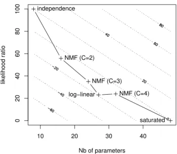
Figure 2 illustrates the well-known trade-off between com-pression and approximation on the Governance cube. The X-axis is the number of parameters in the model (lower means more compression) while the Y-axis is the likelihood ratio (lower means better approximation). The dotted lines are contours of the AIC. An ideal model with good approx-imation using few parameters would be in the bottom left corner.

From this figure, one can see that the independence and

saturated models are two extremes, and other probabilistic

models are positioned in between. Moreover, as the num-ber of NMF components increases, the approximation im-proves, but the number of parameters grows. One model that reaches a good compromise between compression and approximation is the 3-component model, which has the best AIC of all NMF models. Note that the parsimonious log-linear model reaches a different, and seemingly better (for

that cube) compromise.

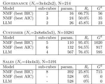
In order to empirically analyze the trade-off between com-pression and approximation, we consider our three example cubes and three models (NMF with BIC, NMF with AIC and LLM), and compute for each model the compression rate Rc(Equation 5) and the deviance G2.

Table 3 shows that in the Governance cube, all models compress the data by one half to two-third. The Customer cube compresses well, from 76.4% for LLM to about 95% for

10 20 30 40 0 20 40 60 80 100 Nb of parameters likelihood ratio independence NMF (C=2) NMF (C=3) log−linear NMF (C=4) saturated

Figure 2: The compression-approximation trade-off for the Governance cube.

NMF. Finally, the Sales cube is harder to compress. Using BIC, the NMF yields a compression rate of only 26% for the third cube, while LLM does not manage to compress the data since there exists a three-way interaction between the three existing dimensions.

These experimental results confirm that BIC yields a more parsimonious representation than AIC. This is known from theoretical considerations, as the BIC penalty is larger. How-ever, results also seem to indicate that NMF tends to com-press the data more than LLM. This comes of course at the price of a worse approximation, as indicated by G2 _{in Table} 3. In all cases, the deviance is much larger for the BIC-optimal NMF than for the AIC-BIC-optimal NMF and LLM, indicating a worse fit.

These results suggest that NMF and LLM are able to bal-ance the conflicting goals of compression and faithful rep-resentation of the data in different ways and to different degrees, with LLM focusing more on good approximation, while NMF produces more compact representations of the data. In the most extreme case presented here, the BIC-optimal NMF represents the 2400 cells of the Customer cube using only 109 free parameters. This represents a very large space saving.

The approximation of cubes allows also a better under-standing and an easier exploration of data as indicated be-low.

4.3 Approximate Query Answering

In this section, we show how OLAP queries [8] may be an-swered within the NMF framework using information about the generated components. We consider the following op-erators: selection (Dice), projection (Slice) and aggregation (Roll-Up). Many other OLAP operators (Rotate, switch, etc.) are concerned primarily with visualization and/or per-mutations of dimensions and modalities, and therefore do not carry any significant change to the model.

A Roll-up will aggregate values either over all the ities of one or several dimensions, or over subsets of

(8)

modal-Governance(Nc=3x4x2x2), N=214

Model sub-cubes param. Rc G2

NMF (best BIC) 2 16 66.7% 56

NMF (best AIC) 3 24 50.0% 35

LLM 2 26 45.8% 23

Customer(Nc=2x8x6x5x5), N=10281

NMF (best BIC) 5 110 95.4% 1020

NMF (best AIC) 6 132 94.5% 917

LLM 4 567 76.4% 595

Sales(Nc=44x4x3), N=5191

NMF (best BIC) 8 392 25.8% 715

NMF (best AIC) - 528 0% 0

LLM - 528 0% 0

Table 3: Output of NMF and LLM for three differ-ent data cubes. Ncis the number of cells in the table, N is the number of records, Rc is the compression rate, and G2 _{is the deviance.}

ities. This is easily implemented on the model by summing over the corresponding probabilistic profile. In addition, when a roll-up is performed over all modalities of a dimen-sion, by definition the sum over the entire probabilistic pro-file is 1, i.e. PkP (k|m) = 1, meaning that this probabilis-tic profile is simply dropped from the model. An example will clarify this. Without loss of generality, let us assume a three-dimensional cube X = [xijk] with corresponding 3D NMF model Px(i, j, k) =

P

mP (m)P (i|m)P (j|m)P (k|m). A roll-up over dimension k will result in a 2-dimensional cube Y = [yij]. The corresponding NMF model is Py(i, j) = P k P mP (m)P (i|m)P (j|m)P (k|m) = P mP (m)P (i|m)P (j|m). The model estimate for the rolled-up cube Y is therefore ob-tained “for free” from the model of the original cube X with essentially no additional computation. Note that the result-ing model for cube Y is not optimal in the sense that it does not necessarily maximize the likelihood on that cube. However, the resulting estimated counts byij = N.Py(i, j) (with N = P_ijkxijk) are exactly the same as what we would obtain by first forming the estimated cube for X us-ing bxijk = N.Px(i, j, k), and doing a roll-up on that cube. Doing the roll-up on the model lightens the computational requirements. In the example given above, instead of order 4.M.I.J.K operations3for forming the entire cube and I.J.K for the aggregation operation, only 3.M.I.J operations are required.

The Slice and Dice operations are similar in the sense that they select a portion of the cube and differ mainly on the extent of the selection. The availability of a probabilistic model potentially cuts the processing in at least two ways. First, only the necessary cells may be approximated, instead of computing the entire approximate cube and performing the Slice or Dice explicitly on the full cube. Second, during the approximation, it is possible to discard the components that are not relevant to the current query.

As an illustration we will use the NMF model of five com-ponents selected by BIC for the Customer cube. Table 4 3_{Recall that M stands for the number of components.}

Modalities Dimension Data C1 C2 C3 C4 C5 Status 1, 2 1, 2 1, 2 1, 2 1, 2 1, 2 Income 1-8 4-8 1-3 1-3 2, 3 1-4, 6, 8 Child 0-5 0-5 0-5 0-5 0-5 0-5 Occupation 1-5 4, 5 1-5 1, 2 1, 2 4, 5 Education 1-5 1-5 3 1, 2 1-3 4, 5

Table 4: Modalities of the 5-dimensional data cube “Customer” and its five components C1 to C5. The following convention is used: i, j means that only modalities i and j are non-zero for the correspond-ing dimension and component, and i − j means all modalities between i and j.

shows modalities of the Customer cube and its five compo-nents C1 to C5. The table shows, for each component, the modalities of each dimension that are “active”, i.e. have a probability significantly higher than zero. For example, in component C2, all values of Occupation are probable, but for components C3 and C4, values of Occupation higher than 2 have a zero probability. This table will be helpful in the design of our OLAP query plans. For example, when the query involves cells with Income=3, component C1may be ignored; for Occupation=3, the only relevant component is C2.

Let us consider the following queries:

1. Slice: Number of customers according to Status, In-come, Child, and Occupation for customers with Education= 4 (bachelor’s degree).

2. Dice: Number of customers according to Status, In-come, and Occupation for customers with Educa-tion= 4 (bachelor’s degree) or 5 (graduate studies) where Child ∈ {3, 4, 5}.

3. Roll-U p1: Number of customers according to Income, Occupation, and Education (a subset of dimensions of the Customer cube).

4. Roll-U p2: Number of customers according to the five dimensions (Status, Income, Child, Occupation and Education) with a roll-up on the Income hierarchy (e.g., three intervals: 1-3, 4-5, and 6-8).

The first two queries are processed using only components C1and C5—all other are zero for Education=4 or Educa-tion=5. The Dice query can then be processed as follows: (i) perform Dice query (i.e., selection on Education and Child) on C1 to get C′1; (ii) compute, into C5′, the number of customers according to Status, Income, and Occupa-tion for customers with Child ∈ {3, 4, 5}; (iii) add C′

1 to

C′

5 to get the approximate answer.

For the third query, a three dimensional model is available directly from the original five dimensional NMF by dropping the profiles for Child and Education from the model. All five components are used, but for three dimensions only.

Finally, the fourth query concerns a roll-up on the hier-archy of the Income dimension. It can be answered by se-lecting the appropriate components and aggregating data for each interval of Income. In that way, irrelevant components can be ignored for each interval of Income (component C1 for interval 1-3, and C2 to C4for 4-5 and 6-8).

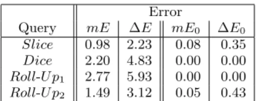
Table 5 reports mean (mE) and standard deviation (∆E) of the approximation error (absolute difference) observed

(9)

Error

Query mE ∆E mE0 ∆E0

Slice 0.98 2.23 0.08 0.35 Dice 2.20 4.83 0.00 0.00 Roll-U p1 2.77 5.93 0.00 0.00 Roll-U p2 1.49 3.12 0.05 0.43

Table 5: Mean (mE) and standard deviation (∆E) of the absolute error by cell. mE0 and ∆E0 are the mean and standard deviation on the cells with zero count.

between the result of each query performed on the original data, and the approximation calculated as presented above, directly on the model. We also check whether the model approximates well empty cells in the cube by calculating the approximation error limited to these empty cells (mE0 and ∆E0).

Table 5 shows that, mean absolute error by cell (mE) is the smallest for Slice query. This situation is explained by the fact that Slice query processing does not need cells aggre-gation which implies error accumulation. In Roll-U p2query, error is partially accumulated since a partial aggregation is performed while building intervals on Income. (mE0) and (∆E0) values are very small, which indicates that zero-cells are generally well-estimated.

5. DISCUSSION

The present work shows that NMF and LLM display sim-ilarities and differences. As NMF and LLM are probabilistic models, they associate a probability to each cell in the data cube. This is very helpful to detect outliers by comparing the observed count in one cell with the expected frequency according to the modeled probability (see [15, 24]).

Both models break down a complex data analysis problem into a set of smaller sub-problems. In the context of data warehousing, this means that instead of exploring a large multi-dimensional data cube, the user can analyze a few sets of smaller cubes. This reduces distracting and irrelevant elements and eases the extraction of actionable knowledge.

NMF can identify homogeneous dense regions inside a sparse data cube and find relevant modalities within each dimension for each sub-cube. LLM, on the other hand, can identify important correlations between dimensions. While NMF expresses the original data cube as a superposition of several homogeneous sub-cubes, LLM expresses the origi-nal data cube as a decomposition into a set of sub-cubes expressing strong associations among dimensions. In both cases, the sub-cubes allow the user to focus on one partic-ular component/association at a time rather than on the population as a whole.

Although both models can handle a variety of multi-way arrays, there are also key differences in the way they use their parameters [15]. In NMF, the number of parameters scales linearly in the number of components, and the scaling factor is the sum of the number of modalities on all dimen-sions (up to a small constant, e.g., I + J + K − 2 for three dimensions). On the other hand, the number of parame-ters in LLM depends on lower-order products of the number of modalities in each of the dimensions involved in the re-tained interactions. As a consequence, LLM is better suited for modeling tables with many dimensions, each with

rela-tively few modalities, like in some data cubes. NMF will get the largest benefits from situations where there are relatively few dimensions, each with large numbers of modalities, such as textual data.

6. CONCLUSION

In this paper we advocate the use of non-negative multi-way array factorization for the approximation, compression and exploration of data cubes. We also compare this tech-nique with log-linear modeling for cube approximation and compression. Both techniques reach a compromise between smaller memory footprint and good approximation. Finally, we show how NMF can handle OLAP query answering by se-lecting the appropriate components to consider. This is par-ticularly useful for queries involving selection and/or roll-up on dimensions.

Our future work concerns the following topics: (i) im-prove the efficiency of the model selection and parameter estimation procedures in order to scale up to very large data cubes, (ii) incrementally update an NMF model when a set of aggregate values are added to the data cube such as a new dimension or new members of a dimension (e.g., a new month); and (iii) explore and intensively experiment the po-tential of NMF for approximating large data sets, and for preprocessing data to get homogeneous and dense sub-cubes that could then be analyzed individually using LLM for ex-ample.

7. ACKNOWLEDGMENTS

This work was supported in part by the Natural Sciences and Engineering Research Council of Canada (NSERC) un-der the discovery grant PGPIN-48472. The authors would like to thank the anonymous referees for their valuable com-ments and suggestions.

8. REFERENCES

[1] H. Akaike. A new look at the statistical model identification. IEEE Transactions on Automatic

Control, 19(6):716–723, 1974.

[2] J. L. Ambite, C. Shahabi, R. R. Schmidt, and A. Philpot. Fast approximate evaluation of olap queries for integrated statistical data. In Proceedings

of the First National Conference on Digital

Government Research, 2001.

[3] B. Babcock, S. Chaudhuri, and G. Das. Dynamic sample selection for approximate query processing. In

SIGMOD ’03: Proceedings of the 2003 ACM SIGMOD

international conference on Management of data,

pages 539–550, New York, NY, USA, 2003. ACM Press.

[4] D. Barbara and X. Wu. Using loglinear models to compress datacubes. In WAIM ’00: Proceedings of the

First International Conference on Web-Age

Information Management, pages 311–322, London,

UK, 2000. Springer-Verlag.

[5] D. Barbara and X. Wu. Loglinear-based quasi cubes.

J. Intell. Inf. Syst., 16(3):255–276, 2001.

[6] A. Boujenoui and D. Zéghal. Effet de la structure des droits de vote sur la qualité des mécanismes internes de gouvernance: cas des entreprises canadiennes.

Canadian Journal of Administrative Sciences,

(10)

[7] K. Chakrabarti, M. Garofalakis, R. Rastogi, and K. Shim. Approximate query processing using wavelets. The VLDB Journal, 10(2-3):199–223, 2001. [8] S. Chaudhuri and U. Dayal. An overview of data

warehousing and olap technology. SIGMOD Rec., 26(1):65–74, 1997.

[9] R. Christensen. Log-linear Models. Springer-Verlag, New York, 1997.

[10] W. Deming and F. Stephan. On a least squares adjustment of a sampled frequency table when the expected marginal totals are known. The Annals of

Mathematical Statistics, 11(4):427–444, 1940.

[11] A. P. Dempster, N. M. Laird, and D. B. Rubin. Maximum likelihood from incomplete data via the EM algorithm. Journal of the Royal Statistical Society,

Series B, 39(1):1–38, 1977.

[12] I. S. Dhillon and S. Sra. Generalized nonnegative matrix approximations with bregman divergences. In

Advances in Neural Information Processing Systems 17, pages 283–290, 2005.

[13] V. Ganti, M.-L. Lee, and R. Ramakrishnan. Icicles: Self-tuning samples for approximate query answering. In VLDB ’00: Proceedings of the 26th International

Conference on Very Large Data Bases, pages 176–187,

San Francisco, CA, USA, 2000. Morgan Kaufmann Publishers Inc.

[14] E. Gaussier and C. Goutte. Relation between PLSA and NMF and implications. In SIGIR ’05: Proceedings

of the 28th annual international ACM SIGIR conference on Research and development in

information retrieval, pages 601–602, New York, NY,

USA, 2005. ACM Press.

[15] C. Goutte, R. Missaoui, and A. Boujenoui. Data cube approximation and mining using probabilistic

modelling. Technical Report NRC 49284, National Research Council, 2007.

http://iit-iti.nrc-cnrc.gc.ca/publications/nrc-49284 e.html.

[16] S. Haberman. Analysis of qualitative data, Volume 1. Academic Press, New York, 1978.

[17] T. Hofmann. Probabilistic latent semantic analysis. In

UAI’99, pages 289–296. Morgan Kaufmann, 1999.

[18] T. Imielinski, L. Khachiyan, and A. Abdulghani. Cubegrades: Generalizing association rules. Data Min.

Knowl. Discov., 6(3):219–257, 2002.

[19] L. V. S. Lakshmanan, J. Pei, and Y. Zhao. Quotient cube: How to summarize the semantics of a data cube.

In Proceedings of the 28th International Conference on

Very Large Databases, VLDB, pages 778–789, 2002.

[20] D. D. Lee and H. S. Seung. Learning the parts of objects by non-negative matrix factorization. Nature, 401:788–791, 1999.

[21] H. Lu, L. Feng, and J. Han. Beyond intratransaction association analysis: mining multidimensional intertransaction association rules. ACM Trans. Inf.

Syst., 18(4):423–454, 2000.

[22] S. Naouali and R. Missaoui. Flexible query answering in data cubes. In DaWaK, pages 221–232, 2005. [23] T. Palpanas, N. Koudas, and A. Mendelzon. Using

datacube aggregates for approximate querying and deviation detection. IEEE Transactions on Knowledge

and Data Engineering, 17(11):1465–1477, 2005.

[24] S. Sarawagi, R. Agrawal, and N. Megiddo.

Discovery-driven exploration of olap data cubes. In

EDBT ’98: Proceedings of the 6th International

Conference on Extending Database Technology, pages

168–182, London, UK, 1998. Springer-Verlag. [25] G. Schwartz. Estimating the dimension of a model.

The Annals of Statistics, 6(2):461–464, 1978.

[26] J. Shanmugasundaram, U. Fayyad, and P. S. Bradley. Compressed data cubes for olap aggregate query approximation on continuous dimensions. In KDD ’99:

Proceedings of the fifth ACM SIGKDD international

conference on Knowledge discovery and data mining,

pages 223–232. ACM Press, 1999.

[27] J. S. Vitter and M. Wang. Approximate computation of multidimensional aggregates of sparse data using wavelets. In Proceeding of the SIGMOD’99

Conference, pages 193–204, 1999.

[28] M. Welling and M. Weber. Positive tensor factorization. Pattern Recognition Letters, 22(12):1255–1261, 2001.

[29] F. Yu and W. Shan. Compressed data cube for approximate olap query processing. J. Comput. Sci.