An Analysis of the Relationships Between Soil Moisture,
Rainfall, and Boundary Layer Conditions, Based on Direct
Observations from Illinois
by
Kirsten L. Findell
B.S.E., Princeton University (1992)
Submitted to the Department of Civil and Environmental Engineering in
partial fulfillment of the requirements for the degree of
Master of Science in Civil and Environmental Engineering
at the
MASSACHUSETTS INSTITUTE OF TECHNOLOGY
June 1997
© Massachusetts Institute of Technology 1997. All rights reserved.
Signature of Author:
...
...
Department of Civil and Environmental Engineering
S
May 23, 1997
Certified by: ....
Elfatih A. B. Eltahir
Assistant Professor
n Thesis Supervisor
Accepted by: ...
Joseph M. Sussman
Chair, Departmental Committee on Graduate Studies
... .
OF- TEC2* *I..
Eng.
JUN
2
41997
An Analysis of the Relationships Between Soil Moisture,
Rainfall, and Boundary Layer Conditions, Based on Direct
Observations from Illinois
by
Kirsten L. Findell
B.S.E., Princeton University (1992)
Submitted to the Department of Civil and Environmental Engineering on May 23, 1997 in partial fulfillment of the
requirements for the degree of
Master of Science in Civil and Environmental Engineering
Abstract
This study of the soil moisture-rainfall feedback uses a dataset beginning in 1981 of bi-weekly neutron probe measurements of soil moisture at up to 19 stations in Illinois to show that soil moisture can play a significant role in maintaining drought or flood conditions during the summer. Results of a linear correlation analysis between initial soil saturation and rainfall in the subsequent three weeks showed that a positive correlation between these two variables is present from early June through mid-August. This correlation is more significant than the serial
correlation within precipitation time series, suggesting the likelihood of a physical mechanism linking soil moisture to subsequent rainfall.
This result prompted further investigation into the nature of such a physical pathway linking soil moisture to subsequent rainfall. Near-surface hourly observations of pressure, P, temperature, T, wet-bulb temperature, T., and relative humidity,f, from 13 stations in and close to Illinois were used in these analyses. From each hourly set of direct observations of P, T, Tw, andf, wet-bulb depression, Tdpr, temperature of the lifting condensation level (LCL), TLCL, pressure depth to the LCL, PLCL-P,, mixing ratio, w, potential temperature, 0, virtual potential temperature, 60, wet-bulb potential temperature, 9, and equivalent potential temperature, OE were computed. Time series of the spatial average of each of these quantities were then calculated by averaging data from the 13 stations at each hour.
An analysis of the connections between an average soil saturation time series for the whole state of Illinois with these state-wide average boundary layer conditions did not yield the
anticipated positive correlation between soil moisture and moist static energy, as quantified by Tw,
0., or OE. It is not clear if this is due to limitations of the data or of the theory. There was
evidence, however, that moisture availability (or lack thereof) at the surface has a very strong impact on the wet-bulb depression of near-surface air, particularly from mid-May through the end of August, showing good correspondence to the period of significant soil moisture-rainfall
The final set of analyses performed included an investigation of hourly boundary layer and rainfall data. Data from the 82 hourly rainfall stations were averaged to compare state-wide hourly rainfall to state-wide hourly boundary layer conditions. A link between high MSE and high rainfall was noted for much of the range of MSE during the summer months, and a link between
low Tdpr and high rainfall was evident for all of the months analyzed (April through September).
These analyses, then, suggest that the significant but weak correlation between soil moisture and rainfall during Illinois summers is due not to soil moisture controls on the boundary layer entropy, but rather to soil moisture controls on the wet-bulb depression of near-surface air.
Thesis Supervisor: Elfatih A. B. Eltahir
Acknowledgments
There are many individuals who have contributed in countless ways to my academic and
personal growth since I've been at MIT. Thanks are due to my advisor, Elfatih Eltahir, both for
his guidance and feedback on this work, and for his willingness to welcome me into his researchl
group. I am forever grateful to Dennis McLaughlin for his enormous patience with me when I
was blindly searching for the research discipline that was right for me. His advice, support and
understanding are still appreciated more than he can know.
Many people at the Parsons Lab have helped to make this place a warm and welcoming
second home, but a few people deserve special recognition for their companionship and laughter.
Jeremy Pal, for all the soil moisture conversations, for his insights and theories on human nature,
and, of course, for his computer expertise. Sanjay Pahuja for the plants, the stories, the yoga, the
bibliography, and for his ability to find the beauty in everything. Pat Dixon for her warmth and
caring, and for sharing a bit of herself with me. Sheila Frankel for taking care of the lab and for
getting computers in our offices. Cynthia Stewart for making sure that sanity comes before
deadlines. Lynn Reid for her tough big-sisterly love. Tom Ravens, David Senn, Julie Kiang, John
MacFarland, Ida Primus, and Guiling Wang for making me smile every time I see them. And, of
course, Freddi-Jo Eisenberg for being my biographer and soul-mate.
Thanks also go to John Hansman for the runs, swims, and conversations: he has helped
diffuse many headaches and frustrations; to Laura and Hans Indigo for their friendship and
support, and for helping to give me a life outside of MIT; to Miriam Bowling for laughing with
me and helping me keep things in perspective; to my amazing sister Leanne for always believing in
me and knowing just when to tell me so; to my brother Kent and my mother Carol for the open'
doors whenever I need an escape from the city; to my father George for his belief that I can do
anything I want to do; to my house mates Becky Frank and Susan Kaplan for helping to make our
house a home; and especially to my yoga teachers extraordinaire, Gurucharan Singh Khalsa and
Hari Kaur Frank for helping me take care of myself and always encouraging me to keep up!
Steven Hollinger, Randy Peppler, Tami Creech, and Jim Angel of the Illinois State Water
Survey were kind enough to contribute their soil moisture and precipitation data to this study.
Special thanks go to Jim Angel for responding to my last-minute request for digital information on the Illinois state line.Much appreciation also goes to the National Science Foundation for supporting me with a Graduate Student Fellowship.
Table of Contents
Chapter 1: Introduction ... ... 9
Chapter 2: The Role of Soil Moisture in the Climate System... ... 12
A. Background and Theory ... 12
B. Previous Data Analyses ... 17
C. GCM Results ... 22
D. Results of Regional Climate Studies ... 24
Chapter 3: The Relationships Between Soil Saturation and Subsequent Rainfall...28
A. Soil Moisture Data ... .28
B. Daily Precipitation Data ... 34
C. Results and Discussion: The Interplay Between Soil Saturation and Subsequent Precipitation Throughout the Year ... 35
D. Results and Discussion: Focus on Spring and Summer Connections ... 42
E. Discussion of Results ... 46
Chapter 4: The Relationships Between Soil Saturation and Boundary Layer Conditions...48
A. The NCDC Surface Airways Hourly Dataset... ... 48
B. Presentation of Results ... 50
C. Analysis of Initial Soil Saturation Followed by 21-Day Average of Boundary Layer Conditions, Averaged Over All of Illinois ... 52
D. Analysis of the Linear Correlation Between Soil Saturation and Subsequent Boundary Layer Conditions Throughout the Year... ... 79
E. Discussion of Results ... 87
Chapter 5: The Relationships Between Boundary Layer Conditions and Rainfall ... :90
A. The EarthInfo NCDC Hourly Rainfall Database...90
B. The Diurnal Cycle of Rainfall in Illinois. ... 90
C. Analysis of Afternoon Storm Events and the Preceding Boundary Layer Conditions ... ... 97
D. Discussion of Results ... 132
Chapter 6: Conclusions and Future Research ... 136
List of Figures
Figure 3.1: Locations of Illinois State Water Survey (ISWS) soil moisture stations and rainfall stations. Solid line is the Illinois state boundary ... ... 29 Figure 3.2: Annual average of soil saturation cycles for each year, 1981-1994. Dashed line is
1988 (extreme drought); solid line is 1993 (extreme flood); all other years are drawn with dotted lines; thick dotted line is average of all 14 years; a) top 10 cm, b) top 30 cm, c) top
50 cm, d) top 70 cm, e) top 90 cm, f) top 1.1 m. ... ... 32 Figure 3.3: Seasonal average soil saturation profiles: a) December-February (DJF), b)
March-May (MAM), c) June-August (JJA), d) September-November (SON). Left-most solid line is 1988 (extreme drought); right-most solid line is 1993 (extreme flood); all other years are drawn with dotted lines; dashed line is average of all 14 years... 34 Figure 3.4: Average total monthly precipitation over Illinois, 1981-1994. Stars indicate means of
the 14 years; lines extend to plus or minus one standard deviation. ... 35 Figure 3.5: Linear correlation between initial soil saturation and precipitation in the subsequent
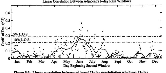
21 days for a) top 10 cm, b) top 50 cm, and c) top 90 cm. Solid line is 21-day moving average. Level of significance lines refer to the daily values (not the smoothed line)...37 Figure 3.6: Linear correlation between adjacent 21-day precipitation windows; 21-day
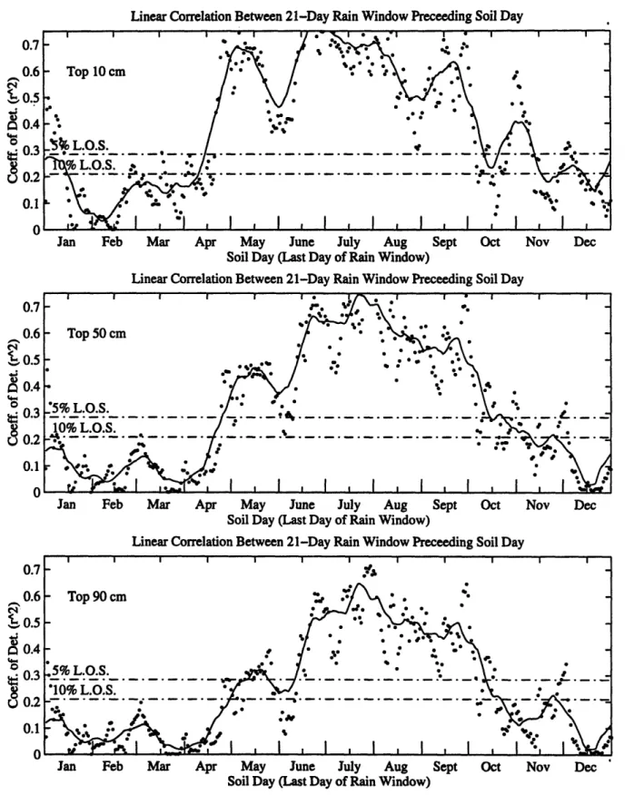
smoothing. Solid line is 21-day moving average. Level of significance lines refer to the daily values (not the smoothed line)... 38 Figure 3.7: Linear correlation between 21-day total precipitation and soil saturation at the end of
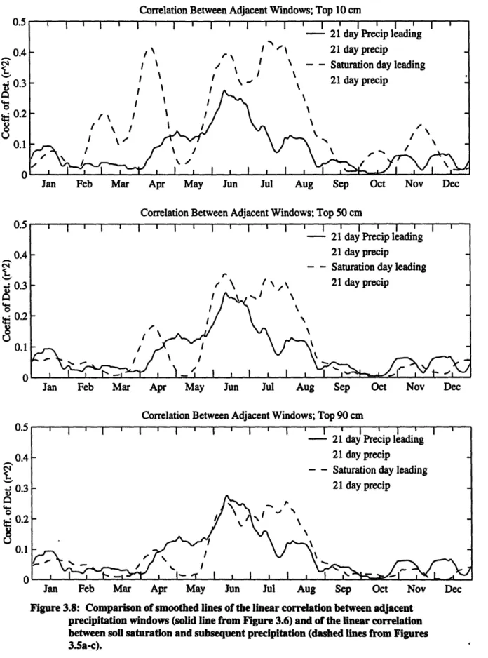
the 21 days for a) top 10 cm, b) top 50 cm, and c) top 90 cm. Solid line is 21-day moving average. Level of significance lines refer to the daily values ... 40 Figure 3.8: Comparison of smoothed lines of the linear correlation between adjacent precipitation
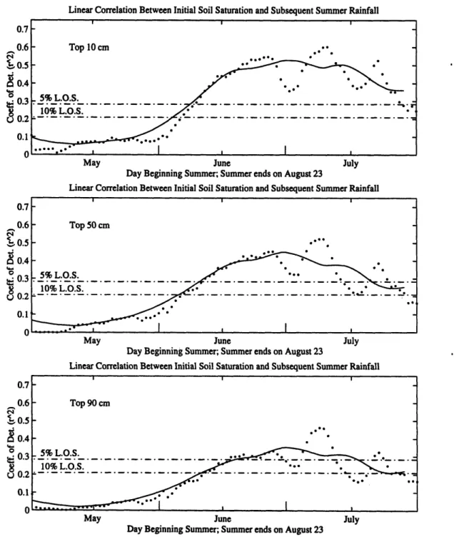
windows (solid line from Figure 3.6) and of the linear correlation between soil saturation and subsequent precipitation (dashed lines from Figures 3.5a-c). ... 41 Figure 3.9: Linear correlation between initial soil saturation and precipitation in the rest of the
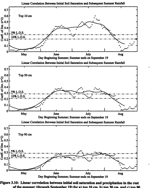
summer (through August 23) for a) top 10 cm, b) top 50 cm, and c) top 90 cm. Solid line is 21-day moving average. Level of significance lines refer to the daily values (not the sm oothed lines) ... ... 43 Figure 3.10: Linear correlation between initial soil saturation and precipitation in the rest of the
summer (through September 19) for a) top 10 cm, b) top 30 cm, and c) top 90 cm. Solid line is 21-day moving average. Level of significance lines refer to the daily values (not the smoothed lines)... 44 Figure 3.11: Average Initial soil saturation on June 25 for a given year versus summer (July 1 to
August 23) precipitation for each year. Numbers beside each data point indicate sample year. Dotted lines are means of the 14 years ± one standard deviation, separating data into low, normal, and high categories of soil saturation and summer precipitation ... 45 Figure 4.1: Locations of ISWS soil moisture stations and NCDC Surface Airways Hourly Dataset
Figure 4.2: Soil saturation (SS) and maximum daily temperature (7) for days during July, during the years 1981 to 1995; a) scatter plot of all data pairs; b) probability density functions (PDFs) for three subsets of the data based on the degree of soil saturation; c) first
moments of the PDFs in 4.2b; d) cumulative distribution functions (CDFs) for the PDFs in
4.2b ... 50
Figure 4.3: First moments and Cumulative Distribution Functions (CDFs) of 21-day mean of maximum relative humidity (f), given that soil saturation (SS) on the day prior to the averaging window is low, medium, or high. Note that April, May and September plots are on one scale, while June, July and August plots are on a different scale: a) April, b) May, c) June, d) July, e) August, f) September ... 54
Figure 4.4: As in Figure 4.3, but for mixing ratio (w); a) April, b) May, c) June, d) July, e) August, f) September. ... ... 57
Figure 4.5: As for Figure 4.3 but for air temperature (T); a) April, b) May, c) June, d) July, e) August, f) September. ... ... 59
Figure 4.6: As for Figure 4.3 but for wet-bulb temperature (Tw); a) April, b) May, c) June, d) July, e) August, f) September ... 63
Figure 4.7: As for Figure 4.3 but for wet-bulb depression (Tdp,); a) April, b) May, c) June, d) July, e) August, f) September ... 66
Figure 4.8: As for Figure 4.3 but for temperature of the lifting condensation level (TIc1); a) April, b) May, c) June, d) July, e) August, f) September ... 69
Figure 4.9: As for Figure 4.3 but for pressure depth to the lifting condensation level (P1,c -P,); a) April, b) May, c) June, d) July, e) August, f) September ... 72
Figure 4.10: As for Figure 4.3 but for equivalent potential temperature (OE); a) April, b) May, c) June, d) July, e) August, f) September ... ... 75
Figure 4.11: As for Figure 4.3 but for wet-bulb potential temperature (0w); a) April, b) May, c) June, d) July, e) August, f) September ... 77
Figure 4.12: Linear correlation between initial soil saturation (SS) and average (a) minimum daily, (b) mean daily, and (c) maximum daily relative humidity (f) in the subsequent 21 ' days, as measured by the coefficient of determination (2). Solid line is 21 day moving average. "LOS" lines are 5 and 10% level of significance lines for the r2 variable (not the sm oothed line). ... ... 81
Figure 4.13: As for Figure 4.12, but for wet-bulb depression (Tdr). ... 82
Figure 4.14: As for Figure 4.12c but for maximum daily mixing ratio (w) ... 83
Figure 4.15: As for Figure 4.12c but for maximum daily air temperature (7) ... 83
Figure 4.16: As for Figure 4.12c but for maximum daily wet-bulb temperature (Tw). ... 83
Figure 4.17: As for Figure 4.12c but for maximum daily temperature of the lifting condensation level (TLCL) ... ... 84
Figure 4.18: As for Figure 4.12c but for maximum daily pressure depth to the lifting condensation
level (PL L -Ps) ... ...84
Figure 4.19: As for Figure 4.12c but for maximum daily equivalent potential temperature (OE)...85
Figure 4.20: As for Figure 4.12c but for maximum daily wet-bulb potential temperature (w)...85 Figure 4.21: As for Figure 4.12c but for initial soil saturation in the top 50 cm and average
maximum daily wet-bulb depression (Td,,) in the subsequent 21 days ... 86 Figure 4.22: As for Figure 4.12c but for initial soil saturation in the top 90 cm and average
maximum daily wet-bulb depression (Td,,) in the subsequent 21 days ... 86 Figure 5.1: Locations of the NCDC Hourly Rainfall Stations (*) and the NCDC Surface Airways
Stations (o). Solid line is the Illinois state boundary... ... 91 Figure 5.2: The diurnal cycle of rainfall depth, storm duration, and probability of initiation for
April and May; June and July; August and September...94 Figure 5.3: Correlations between hourly pressure (P) and rainfall during April and May; June and July; August and September... 98 Figure 5.4: Correlations between hourly relative humidity (f) and rainfall during April and May;
June and July; August and September ... 102 Figure 5.5: Correlations between hourly mixing ratio (w) and subsequent rainfall during April and
May; June and July; August and September ... 105 Figure 5.6: Correlations between hourly wet-bulb temperature (Tw) and rainfall during April and
May; June and July; August and September ... 111 Figure 5.7: Correlations between hourly wet-bulb potential temperature (G0) and subsequent
rainfall during April and May; June and July; August and September ... 114 Figure 5.8: Correlations between hourly wet-bulb depression (Tdp,,) and subsequent rainfall
during April and May; June and July; August and September... 117 Figure 5.9: Correlations between hourly temperature of the lifting condensation level (TLcL) and
subsequent rainfall during April and May; June and July; August and September. ... 120 Figure 5.10: Correlations between hourly pressure depth to the LCL (P~L -P,) and rainfall
during April and May; June and July; August and September... 123 Figure 5.11: Correlations between hourly equivalent potential temperature (OE) and rainfall
during April and May; June and July; August and September... 126 Figure 5.12: Correlations between hourly air temperature (7) and subsequent rainfall during April and May; June and July; August and September. ... 129
Chapter 1: Introduction
It has long been recognized that soil moisture plays an important role in regional climate systems through its effect on the partitioning between sensible and latent heat fluxes and on the albedo of the surface. Early work by Namias (1952, 1960, 1962) showed that spring precipitation and soil moisture can impact summer precipitation in the interiors of continents. More recently, many researchers have noted the negative correlation between soil moisture states and mean and maximum temperatures (Karl, 1986; Georgakakos et al., 1995; Huang et al., 1996), and stressed the potential increase in surface heating and decrease in local evaporative contributions to
atmospheric humidity that anomalously low soil moisture states can affect (Rind, 1982; Trenberth, 1988; Oglesby, 1991). Recent work by Williams and Renno (1993) and Eltahir and Pal (1996) suggests a link between rainfall and surface wet bulb temperature during convective rainfall storms in the tropics. Wet bulb temperature is an indicator of surface conditions, including, among other variables, soil moisture. Afternoon storms during the summer months in the
Midwestern United States are thought to be of a similar convective nature as tropical storms. As stated in early work by Carlson and Ludlam (1966), during the summer "the tropical
cumulonimbus convection and its own nearly-neutral stratification tend to advance into higher latitudes."
Many recent studies involving General Circulation Models (GCMs) have offered support to Namias' hypothesis, showing that changes in the soil moisture regime at the end of
spring/beginning of summer can significantly impact summer precipitation over continental land masses (Shukla and Mintz, 1982; Rowntree and Bolton, 1983; Rind, 1982; Yeh et al., 1984; Oglesby and Erickson, 1989; Oglesby, 1991; Fennessy and Shukla, 1996). These GCMs, however, have all been rather broad-brush, making global or continental-scale soil moisture changes. Regional climate studies (Pan et al., 1995; Georgakakos et al., 1995; Huang et al.,
1996; Pal and Eltahir, 1997, for example) have also been used to test this hypothesis regarding the feedback from soil moisture to the atmosphere. The FIFE experiment in Kansas provided some short-term real data with which to test the soil moisture-rainfall feedback. Both Betts et al. (1996) and Eltahir (1997) find a positive feedback relationship between soil moisture and
boundary layer conditions. However, due to a lack of adequate long-term data on soil moisture, no models have been tested against any directly observed, long-term soil moisture data sets.
This study attempts to fill this gap by analyzing the relationship between precipitation and soil moisture using the Illinois Climate Network (ICN) data set: a record of soil moisture values measured bi-weekly at 19 stations across the state of Illinois since 1981 (Hollinger and Isard,
1994). Though this data set is somewhat limited in both temporal and spatial extent, it is the largest available data set of its kind and its analysis should prove worthwhile. If, as many GCM and regional studies results suggest, spring soil moisture does indeed affect summer precipitation, the data should support this hypothesis.
To make this data analysis comparable to modeling studies, the framework for the analysis is posed as an initial value problem. We are interested in how precipitation responds to an initial soil moisture condition. In contrast to a computer model, it is difficult to isolate these two variables when dealing with real data. Nevertheless, the 14 years of data (1981-1994) are more
than has previously been available for this kind of analysis, and could provide some insight into the coupled land-atmosphere system. Furthermore, this analysis, based on actual observations, should provide a testing framework for future numerical experiments involving soil water and precipitation.
After a more detailed discussion of the literature on these processes and on previous data , analyses and modeling experiments, this hypothesis will be tested in Chapter 3 by analyzing 14 years of data on soil moisture and subsequent rainfall in Illinois. As predicted by the theory herein, a positive but weak correlation was found during the summer months. This correlation' prompted the investigation of the correlations between soil moisture and subsequent boundary layer conditions in Chapter 4, where we expected to see evidence of increased soil moisture being followed by increase BLE. This expectation was not met. It is not clear if this is due to
limitations of the data or of the theory. Though this soil moisture-BLE link was not observed, there was evidence that high soil moisture is likely to be followed by low wet-bulb depression,
Tdpr, particularly during the summer.
The next phase of analyses, presented in Chapter 5, focused on the link between boundary layer conditions and rainfall using hourly data. Indeed, a link between high MSE and high rainfall was noted for much of the range of MSE during the summer months, and a link between low Tdpr and high rainfall was evident for all of the months analyzed (April through September). These analyses, then, suggest that the significant but weak correlation between soil moisture and rainfall during Illinois summers is due not to soil moisture controls on the boundary layer entropy, but rather to soil moisture controls on the wet-bulb depression of near-surface air.
Chapter 2: The Role of Soil Moisture in the Climate
System
A.
Background and Theory
Atmospheric dynamics over oceans are quite different from those over land. Water has a much larger heat capacity than soil, and the oceans act as a reservoir for heat and energy. As a result, the diurnal temperature fluctuations that can be enormous over dry land masses like deserts are reduced to just a few degrees over oceans. Similarly, seasonal shifts in mean temperature are much reduced over oceans as compared to lands.
Evaporative processes at the surface of oceans are also quite different from those over land. Evaporation occurs when three things are available: 1) moisture, 2) energy to convert liquid water to water vapor, and 3) a transport mechanism to carry saturated air away from the moisture source. Over open water, moisture is never in short supply, while over land it can often be the limitation on evaporation. When evaporation is limited, regardless of the controlling mechanism, incoming energy is dissipated by the less efficient mechanism of sensible heat flux, which leads to a rise in air temperature. Indeed, it is this difference between the oceanic and land surface ratios of sensible to latent (evaporative) heat flux which is responsible for the larger temperature fluctuations over land. Parched ground has no moisture available for evaporation, so all of the available energy goes to sensible heating of the air, and the air temperature quickly rises. Over a body of water, on the other extreme, evaporation, E, occurs at the potential rate (a function of the
other two limiting factors, energy and transport mechanisms), and much less energy is available for sensible heat transfer.
The amount of moisture in the soil controls where the energy balance of the surface lies in relation to these desert and ocean extremes. This is quantified by the Bowen ratio, P, which is
defined as the ratio of sensible heat flux, H, to latent heat flux, AE, where A is the latent heat of vaporization. Both terms have units of energy flux (W/m2 in S.I. units). Typical values of
3
are on the order of 0.07 over open oceans, where the sea surface temperature responds little to the diurnal cycle of solar forcing (Betts et al., 1996), to many hundreds over dry land surfaces, where all of the energy transfer occurs as sensible heating (e.g. dry lake bed example in Wallace and Hobbs, 1977, p. 345). During the night over land, both H and AE are very small because the land responds quite quickly to the disappearance of solar forcing. The sensible heat flux is often directed downward at night when a temperature inversion is present, so the Bowen ratio may be negative in sign.The comparison of land surface and oceanic controls on atmospheric dynamics is an extreme example of the potential role that soil moisture could play in effecting local weather and climate. An increase in soil moisture increases the heat capacity and thermal conductivity of the
land surface, thereby increasing its thermal stability (McCorcle, 1988). Furthermore, if water availability is the limitation on evaporative exchange, then an increase in soil moisture would allow for an increase in the production of latent heat and a decrease in the production of sensible heat. This mechanism is important in dry to normal conditions, but above some threshold of moisture availability, energy input or transport of saturated air away from the moisture source become the controlling factors on evaporation. Increasing soil moisture beyond this point will not
affect the Bowen ratio. Since this threshold moisture level is variable due to the variability of winds (the transport mechanism) and incoming solar radiation (the energy source), it generally appears in data only as decreased sensitivity, rather than a clear cut-off level, of the Bowen ratio
to moisture availability at high moisture contents.
Another important aspect of the influence of soil moisture on land-atmosphere interactions are the time scales of the many components of the land-atmosphere system. Because the thermal mass of water is so large, oceans respond slowly-with lags on the order of a season-to changes in radiative or other forcing, and they only respond to the low frequency variability. Similarly, soil moisture acts like a reservoir of water which damps out high frequency fluctuations and increases the memory of the land surface system (Entekhabi et al., 1996). This memory bank is an
important aspect of the feedback loop between the land surface and the atmosphere.
Theories abound on the role that soil moisture plays in the moisture and energy budgets of the boundary layer (e.g., Betts et al., 1996; Entekhabi et al., 1996; Eltahir, 1997). They all agree that soil moisture is an important component of the system, but there is disagreement on the relative strengths of the many different ways which soil moisture can effect the boundary layer. These differences will be discussed in the next section. In this section, we will simply sketch the broad outline of the soil moisture-rainfall feedback.
When a stove-top pot is heated from below, energy is added to the lowest levels of the fluid. This begins to generate turbulence and turbulent heat flux away from the heat source, and to create an instability where relatively cold, dense, low energy fluids are overlying relatively warm, less dense, high energy fluids. Turbulence acts to mix these fluids and create uniform profiles of temperature and energy throughout the range of the turbulent activity. As more heat is
added to the system, the strength of the turbulence grows and the depth of the mixed layer grows until the whole pot is boiling and well mixed.
Since the atmosphere is largely transparent to solar radiation, the main heat source for tropospheric air is the land surface. The system acts much like a pot on a stove, with the added complication of the heat associated with phase changes of water (heat is consumed by evaporation and released by condensation). During the day, the temperature of the land surface increases in response to solar forcing, and the corresponding flux of terrestrial radiation increases (this flux is proportional to the fourth power of ground temperature). Net radiation at the surface, R,, is the sum of incoming short wave solar radiation, outgoing long wave terrestrial radiation (negative in sign), and incoming long wave radiation returned to the surface by backscattering off of molecules in the atmosphere, particularly condensed water in clouds. Some of this net radiation is consumed as heat flux into the ground, G, (usually on the order of 15% or less, [Betts et al., 1996]). The remainder, and typically the greater percentage, of R,, is transferred to the air, partly as sensible
heat, and partly as latent heat: R,et -G = H + AE. Both the turbulent sensible and latent heat
fluxes increase the moist static energy (MSE) of the boundary layer (Betts et al., 1996; Carlson and Ludlam, 1966), and mix the lower levels of troposphere so that quantities like mixing ratio and potential temperature are nearly constant throughout this mixed layer. MSE is very closely related to the entropy variable equivalent potential temperature, OE (Emanuel, 1994), and the terms moist static energy and boundary layer entropy (BLE) are used almost interchangeably. Temperature, T, is not constant in the mixed layer because the pressure, P, decreases nearly hydrostatically with increasing height. Potential temperature, 0, accounts for the P dependence of
T: it is defined as the temperature a parcel of air would acquire if it were taken dry adiabatically to
levels up past their level of free convection (LFC), where they are neutrally buoyant with respect to environmental air. Above the LFC, a parcel is positively buoyant and will rise freely until it reaches the level of neutral buoyancy (LNB), cooling and, after reaching saturation, condensing out water vapor as it goes. Initial saturation occurs at the lifting condensation level (LCL), which is often below the LFC. The LCL is usually the cloud base level, while the LNB is approximately the cloud top. If convection is strong enough, and if enough vapor condenses out, precipitation occurs. Since the primary energy source for the boundary layer growth described here is surface fluxes, which are forced by incoming solar radiation, the convective boundary layer is only present during daylight hours (Wallace and Hobbs, 1977).
Soil moisture plays a role in this process by its effect on the Bowen ratio: i.e., by its effect on the partitioning of sensible and latent heat fluxes. Sensible heat flux is largely responsible for the turbulent mixing of near-surface air, so when sensible heat flux increases the boundary layer grows more rapidly. Since the increase of the moist static energy (MSE) in this mixed layer is proportional to the sum of the latent and sensible heat fluxes, the contribution of MSE from the land surface is not dependent on the Bowen ratio. For a given amount of available energy, R,t
-G, a larger Bowen ratio means more sensible heating of the air, a deeper boundary layer, and
therefore, less MSE per unit depth. Wet soils should lead to a smaller Bowen ratio and, by the same reasoning, more MSE per unit depth.
An additional level of complexity in this soil moisture-moist static energy relationship is suggested by Eltahir (1997). Since soil moisture affects the albedo,
x,
of the surface, for a given level of incoming solar radiation, wet soils will decrease the surface albedo, thereby increasing thewet soils decrease the outgoing terrestrial radiation. In addition, wet soils should lead to
increased water vapor content of the air, so more of this terrestrial radiation should be scattered
back towards the surface (greenhouse effect). Each of these three factors, increased Rner, solar,decreased Rooing terre,,strial, and increased Rincong terrestrial, leads to an increase in net radiation: Ret, = Rnet, so,ar - Rougoing terrestrial + Rmncoming terrestrial. Wet soils, then, should not only increase the moist
static energy per unit depth of boundary layer by their impact on the boundary layer depth, they should also increase the contribution of moist static energy from the surface fluxes of sensible and latent heat by increasing net radiation at the surface.
This basic sketch of the processes leading to convective rainfall suggests that increased soil moisture should lead to increased moist static energy in the mixed layer, which should then lead to increased precipitation. However, the style of convection outlined here is not the only mechanism of rainfall production, particularly in the mid-latitudes. In much of the tropics, local convection is responsible for the majority of rainfall throughout the year. In mid-latitudes, on the other hand, synoptic systems play a highly significant part in rainfall production, particularly during the winter. The convective rainfall discussed here is expected to be important in latitude regimes, such as the state of Illinois, only during the summer months. Even in the mid-latitude summers, the impact of soil moisture anomalies is reduced when synoptic winds are strong (Carlson and Ludlam, 1966; Entekhabi et al., 1996).
B.
Previous Data Analyses
The works of Eltahir (1997), Entekhabi et al. (1996), Betts et al. (1996), Betts and Ball (1995), Williams and Renno (1993), and Carlson and Ludlam (1966), among others, have
contributed greatly to the theoretical understanding of the soil moisture-rainfall feedback. Some of the details of these studies will be discussed here.
As discussed above, the partitioning of available surface energy has many effects on the mixed layer. Dry soil leads to increased sensible heating, which leads to increased air
temperatures and greater parcel buoyancy. This increases the depth of the boundary layer, and parcels must rise higher before reaching saturation at their Lifting Condensation Level (LCL). In addition, the turbulent energy associated with the parcel is increased, so there is more entrainment of air from above the mixed layer. This overlying air tends to have lower entropy, so, as pointed out by Betts et al. (1996), greater turbulence leads to reduction of the rate of entropy increase of the mixed layer. Carlson and Ludlam (1966) highlight the difference the depth of the mixed layer has on the wet-bulb potential temperature, 0w, of the layer. The 0, increases during the normal course of the morning and afternoon through both the increased air temperature from sensible heating and the increased water vapor content from evaporation of water from the land surface. When the ground is dry, the available surface energy, Re,t - G, goes into warming and humidifying a deeper boundary layer. The increase of 08, then, is reduced over dry areas as compared to wet areas. Over moist areas, 60 in a convective layer about 150 mb deep rises by about 2.5 °C per day; over arid regions, the convective layer is usually on the order of 400 to 500 mb deep, and the average daily rise in ,, is on the order of only 0.5 *C per day (Carlson and Ludlam, 1966).
The wet-bulb potential temperature is an important measure which is closely related to convection and precipitation: it is conserved in pseudo-adiabatic transformations, and it defines
the path of a parcel lifted from the surface after it reaches saturation. The wet-bulb potential
temperature, 06, is defined as the temperature of a parcel taken moist adiabatically from itswet-bulb temperature, Tw, to a reference pressure of 1000 mb. Tw and ., are very closely related and are, by definition, on the same pseudo-adiabat. Eltahir and Pal (1996) describe the role of wet-bulb temperature in triggering moist convection. The work of Williams and Renno (1993) shows a linear relationship between wet-bulb potential temperature and the convective available potential energy (CAPE) of surface air parcels, using surface and upper air data from many tropical
locations. They found a zero-CAPE intercept at approximately 22-23 *C. The results of Eltahir and Pal (1996) show a similar linear relationship between wet-bulb temperature and the
probability of afternoon rain in the Amazon, with a zero-probability of rainfall intercept at 22 °C. Ludlam (1980) showed that a 0, of at least 20 OC is required for the buildup of substantial CAPE in western Europe. Dessens (1995) used daily minimum temperature, which generally occurs in the early morning, as an approximation of the Ow in following afternoon. He states that there is a strong correlation between these two variables, and shows that 0, is a good predictor of damage from severe hail storms in France. Zawadzki and Ro (1978) and Zawadzki et al. (1981) used vertical soundings from the Toronto area in summer to show that the mean and maximum precipitation rate are well correlated with parcel convective energy.
Betts et al. (1996) performed much of their analyses in terms of the equivalent potential temperature, OE, of the boundary layer. This variable is related to the entropy of the layer throtigh
the equation (cpd + r, ct) In OE s + Rd ln Po, where Cpd is the heat capacity of dry air at constant
pressure, ci is the heat capacity of liquid water, r, is the total water mixing ratio, Rd is the gas constant of dry air, po is a reference pressure of 1000 mb, and s is the specific entropy, or moist entropy (Emanuel, 1994, p. 120). Both s and OE are conserved in reversible moist adiabatic processes. During daylight hours, OE increases due to the surface flux of both sensible heat and
latent heat. Betts et al. (1996) stress that "this surface flux of GE is proportional to the sum of the [sensible heat flux + latent heat flux], and it is not affected by the Bowen ratio" (p. 7214). The contribution of low GE from above the boundary layer, however, tends to reduce 0E in the layer. The degree to which this entrainment occurs is closely linked to the sensible heat flux from the
surface and the associated deepening of the boundary layer: "if the surface [Bowen ratio] is large, although the surface 0E flux may be unchanged, the large [sensible heat] flux drives more
entrainment, produces a deeper [boundary layer], and the diurnal rise of GE is reduced" (p. 7214).
Using data from the FIFE site in Kansas, Betts et al. (1996) showed that, on days during July and August 1987 which were not substantially affected by precipitation or advection of cold
air, higher soil moisture content was associated with higher mixing ratio, q, throughout the day, lower mean temperature, lower maximum temperature, and higher maximum GE. They state that "some of this shift of GE is associated with the sift of the entire diurnal path to higher q with higher soil moisture, but about half is the result of reduced entrainment of dry low GE into the boundary
layer" (p. 7215).
Earlier work by Betts and Ball (1995) focused on subsets of the FIFE data, determined by rainfall and net radiation. Two of their many analyses are particularly relevant to this study. The first compared all days from June to September, 1987 to "wet" days and to "dry" days. "Wet" days were defined to be those with "significant rainfall during the daytime" (p. 25,682), and constituted 29 days. "Dry" days were "days for which the daytime diurnal cycle was not
disturbed by rain or heavy overcast." (p. 25,682) They defined "overcast" as days with a 3-hour average near-noontime net radiation below a threshold: 450 W/m2 for June, July, and August, and 400 W/m2for September. There were 94 "dry" days in the data set. With these classifications,
they found that increased wetness led to higher maximum OE, higher maximum q, smaller diurnal range in T, and, as expected from their definition of the classifications, lower Ret. These
classifications, however, are not determined from the soil moisture observations, and are therefore quite different from the wet, normal, and dry classifications used in this study.
A subsequent analysis in the Betts and Ball work did partition the data by soil moisture, but they only used the 94 days in the "dry" category described above. This is a critical difference between their study and this work. Within subcategories of the dry data, they found that the Bowen ratio and the pressure depth to the Lifting Condensation Level (LCL) were highly
dependent on soil moisture: larger pressure depths and larger Bowen ratios were associated with drier soils. This was especially true between the two driest categories.
Eltahir (1997) stresses the importance of the control that soil saturation has on the albedo of the surface, in addition to the aforementioned Bowen ratio controls. Since water absorbs more solar radiation than dry soil, the albedo of a land surface is negatively correlated with soil
saturation, particularly in the top 10 cm. This effect then propagates into the surface radiation budget: increased soil moisture should decrease the albedo, which then increases the net solar radiation at the surface. Eltahir showed that increased soil saturation should also increase the net terrestrial radiation by increasing the water content of the atmosphere, which will cause more longwave radiation to be directed back towards the surface, and by decreasing the surface temperature, which will result in a decreased radiation away from the surface. All else remaining equal, then, increased soil moisture should lead to an increase in available energy at the surface. This effect, like that discussed above in connection with the work of Betts et al. (1996), should lead to a positive relationship between soil saturation and the entropy of the boundary layer, by
increasing the surface flux of the sum of latent and sensible heats. Eltahir (1997) showed that FIFE data exhibits a positive relationship between soil saturation and wet-bulb temperature.
C.
GCM Results
In addition to theoretical work and small-scale analyses of observations, much insight into the soil moisture-rainfall feedback has been gained from Global Climate Modeling studies. Shukla and Mintz (1982), tested two global scenarios: a wet-soil case, where evapotranspiration is at all times equal to the potential evapotranspiration, and a dry-soil case, where there is no evapotranspiration. Over almost the entire globe, precipitation in the dry-soil case was much less than precipitation in the wet-soil case; while surface temperatures in the dry-soil case were much higher than in the wet-soil case. They concluded that "surface evapotranspiration, which requires moisture in the soil, is a necessary (though not sufficient) condition for extratropical summer precipitation" (p. 1500).
The importance of the timing of soil moisture anomalies in their affect on other climatic variables is stressed by Oglesby's 1991 study of North American droughts. Reduced soil moisture profiles are introduced into two model runs, one beginning on March 1, and one beginning on May 1. In the May 1 run, most of the initial soil moisture anomaly is maintained throughout the summer, except along the east coast of the continent, showing that "through positive feedbacks, reduced soil moisture can be a self-perpetuating condition" (p. 893). The March 1 run, however, shows that the anomalous condition can, in fact, correct itself. The anomaly is apparent at 20 days only over the central United States, and at 50 days, virtually all of North America is at a normal, moist state. He explains these different behaviors by noting that during winter or early spring, when the March 1 anomaly is introduced, solar insolation is generally less than in late
spring and summer. The two primary direct effects of reduced soil moisture content-reduced local evaporation and increased surface heating-are, thus, expected to be less important in this earlier season, and the anomalous condition can be corrected prior to the onset of the new climatic regime.
Rind (1982) finds similar results in his GCM study of North America. By comparing runs which have initially reduced soil moisture levels across the entire United States to control runs, which have normal soil moisture levels on June 1, Rind found significant temperature increases and precipitation decreases across most of the U.S. The effects were most noticeable in June and least noticeable in August, and most consistent in the interior of the continent, where the oceans had the least influence.
Yeh et. al. (1984) conducted a series of numerical experiments which tested, among other things, the importance of the latitude of soil moisture anomalies. In each of the three latitudinal bands studied, namely 300N-60°N, 0-30*N, and 15OS-15°N, initial saturation of the soil caused
both an increase in local precipitation and cooling of the surface due to increased evaporation. Each of the simulations was run during the driest period for the latitudinal band: 1 July to 30 November for the northernmost region, and 1 January to 31 May for the other two.
The studies of Rowntree and Bolton (1983) and Fennessy and Shukla (1996) both found a positive feedback between soil moisture and precipitation. They determined that the strength of the impact is dependent on the size of the soil moisture anomaly region. Other important factors include the solar forcing and the strength of the background winds and regional circulation. Rowntree and Bolton work in terms of a vertically integrated relative humidity, defined as Q/Qsa, where
Q
is the vertically integrated atmospheric water vapor (in g/cm2), and Qsat is thecorresponding saturation vapor content. This quantity is increased by an increase in
Q,
which can occur when evapotranspiration exceeds precipitation, and it is decreased by a rise in temperature, which leads to an increase in Q,.t. They found that an initial soil moisture anomaly over Central Europe affected the partitioning of turbulent heat fluxes at the ground, which in turn affected the modeled temperature, humidity and rainfall during the following 50 days. The atmospheric humidity was found to be much higher in wet soil cases than in dry soil cases, and "the likelihood of precipitation [was] much increased by the wet surface" (p. 503). Model runs with increased winds and circulation strength showed less response to the soil moisture anomaly.Several studies have focused on the causes of the 1988 U.S. summer drought, studying both sea surface temperatures (SSTs) and soil moisture states. Trenberth et al. (1988) found that large-scale circulation patterns caused by SSTs in the Pacific were the likely primary cause, but' that the low soil moisture conditions at the beginning of and throughout the season probably contributed to the severity and persistence of the drought. Atlas et al. (1993), on the other hand, found that tropical SST anomalies reduced the precipitation in the Great Plains, but did not significantly increase the surface temperatures. Simulations with reduced soil moisture levels, however, both increased surface temperatures and decreased precipitation, accurately
approximating the actual 1988 scenario. Oglesby and Erickson (1989) used the NCAR CCM1 general circulation model to demonstrate that reduced spring soil moisture, like that of 1988, can "amplify or prolong summertime drought over North America" (p. 1375).
D.
Results of Regional Climate Studies
Perhaps of more relevance to this analysis of data from Illinois are results from regional scale climate and/or hydrologic models. Pan et al. (1995) focused their study on the flood of
1993 as well as the drought of 1988. They tested the hypothesis that surface moisture availability provides an additional feedback mechanism, helping to maintain extreme wet or dry conditions. Models of a portion of the Midwestern U.S. showed that when all other climatic variables were simulated as observed in each of the two years of interest, extreme changes in the surface moisture conditions (i.e., 99% of saturation simulated with the temperature, wind, and other boundary conditions observed in 1988; 1% of saturation with the boundary conditions of 1993) significantly altered the total summer precipitation.
However, the study of Giorgi et al. (1996) led to the opposite conclusion. They found that local recycling effects were not important in the development of extreme climatic regimes, and, contrary to the aforementioned studies, that a dry soil initial condition provides for increased sensible heat flux, which contributes greater buoyancy to the air, enhancing convective systems and producing more precipitation. This cycle, then, supports a negative feedback mechanism between initial soil condition and precipitation.
In their regional modeling study of the 1988 and 1993 events over the Midwestern US, Pal and Eltahir (1997) found that the sensitivity of the model to soil moisture initialization was
extremely dependent on the convection scheme used in the model. One convection scheme led to results which were highly dependent on the initial local soil moisture conditions, while a different scheme led to quick equilibration of soil moisture anomalies and showed little precipitation difference between wet and dry model runs.
Similar to the Giorgi et al. (1996) study, Georgakakos et al. (1996) found no evidence of soil water feedback to local precipitation in their study of two 2000 km2 basins in Iowa and
accurately simulate observed daily discharge over a 40 year period in each of the basins. One of the primary forcings to the river discharge was an estimated soil moisture time series: the accuracy of their streamflow series (correlation with observations better than 0.8) suggests that their soil moisture series is good. Though soil moisture was not shown to affect precipitation, there were significant cross-correlations between upper soil water leading daily maximum temperature, especially during periods of extreme (high or low) soil water content.
Huang et al. (1996) created a 62 year (1931-1993) time series of monthly soil moisture data for the entire US using a one-layer soil moisture model. They found that soil moisture is a better predictor of future monthly temperature than is antecedent precipitation, particularly in the interior of the continent during summer.
On the smaller end of the spatial and temporal scales, Chang and Wetzel (1991) were able to model the effects of the spatial variability of vegetation and soil moisture on the development of individual storm events. Given the absence of real soil data, they estimated soil moisture from
an antecedent precipitation index. The Illinois data set is not of high enough spatial or temporal resolution to be adequately compared to the results of Chang and Wetzel.
Each of the works mentioned above help to establish and/or substantiate the theory of why we expect to see a positive feedback between soil saturation and rainfall. The studies mentioned in Sections C and D highlight many attempts to discern the impact of soil water conditions on future climate through the use of numerical models. Analyses of small-scale sites such as FIFE
have provided some real-world applications of these theories. In the following three chapters, we will test the theories presented here by looking at directly observed soil moisture, near-surface air,
and rainfall data from the state of Illinois, and see what these data can tell us about the soil moisture-rainfall feedback. We begin by analyzing soil moisture and rainfall data in Chapter 3. Chapters 4 and 5 will include analyses of the relationships between soil moisture and boundary layer conditions, and boundary layer conditions and rainfall, respectively.
Chapter 3: The Relationships Between Soil Saturation
and Subsequent Rainfall
A.
Soil Moisture Data
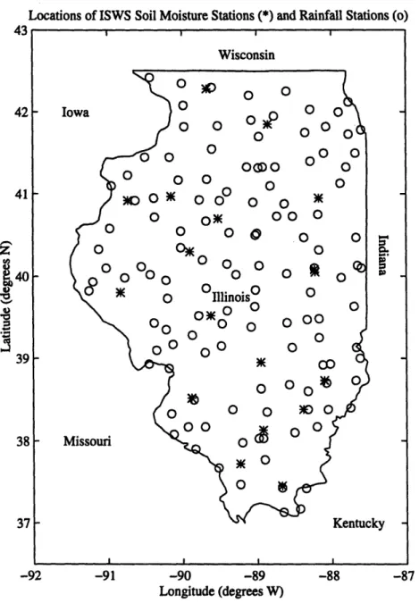
Though each of the studies described in the previous chapter provides analyses of the links between summer rainfall and spring soil moisture, all of them used indirect means to quantify soil moisture. Since 1981, scientists from the Illinois State Water Survey have been taking direct soil moisture measurements with a neutron probe at 8 grass-covered sites around their state (Hollinger and Isard, 1994). Seven additional sites were added in 1982, two more were on-line by 1986, and by 1992, the total was up to 19. Station locations are shown in Figure 3.1. Bi-weekly
measurements were taken in the top 10 cm, in 20 cm intervals between 10 and 190 cm (10-30 cm,
30-50 cm, etc.), and in the 10 cm interval between 1.9 and 2 meters below the surface.
Many researchers (Owe and Chang, 1988; Shukla and Mintz, 1982) have noted the difficulty in obtaining a parameter that represents the soil moisture condition over a whole, large area. Though this data set is a very extensive collection, both temporally and spatially, we must consider the relevance of the parameter measured to this study. According to the hypothesis presented here, the initial soil water condition can provide some positive feedback to the convective regime during the summer months in Illinois. The parameter of interest, then, is the
amount of soil water available for evapotranspiration. The rate at which soil water can be removed is a property of the unsaturated hydraulic conductivity of the soil. Eagleson (1978)
Locations of ISWS Soil Moisture Stations (*) and Rainfall Stations (o) 42 41 39 38 37 -92 -91 -90 -89 -88 -87 Longitude (degrees W)
Figure 3.1: Locations of Illinois State Water Survey (ISWS) soil moisture stations and rainfall stations. Solid line is the Illinois state boundary.
stresses that in exfiltration processes (interstorm drying of the soil as well as extraction by plant roots) it is not the moisture content, q, but rather the soil saturation, q/n, where n is porosity, that is the controlling parameter. Therefore, soil saturation is used as an indicator of the overall soil water condition at each site. Note that this is used as a qualitative indicator of the soil condition, not as an exact measure of the mass of water in the soil: the data are by no means complete
Wisconsin k.. | nl .... . n --- I -v
F
&entucry
enough to offer that level of detail. The soil moisture data, then, were first converted to soil saturations by dividing by the porosity (measurements were made at each of the 19 sites).
Though the sampling frequency (approximately every two weeks) is much greater than for most soil moisture field studies, 14 days is significantly longer than a normal wetting and drying cycle during a Midwestern summer. However, in this study we are not interested in the ability to predict a storm event or exactly describe the soil water condition at every moment in time. Rather, we are concerned with the mean climatic behavior over monthly or seasonal time scales rather than the predictability of erratic weather systems. It is also important to note that the sampling schedule was not set in response to particular storm or drought events (Hollinger, personal communication, 1996). The samples obtained, then, are like random realizations of the ensemble of soil moisture condition at all times throughout the entire state. The assumption implicit in this analysis is that there are enough observations distributed in time and space to give an adequate representation of the trends of the mean soil water condition in the state. An ideal data set for this analysis would have soil moisture sampled multiple times per day at many sites all over the state. Though this data set is not, by this standard, ideal, it is far more complete than any other data set known to date, and much useful information can be gleaned from it.
Simple linear interpolation was used to develop a daily time series of soil saturation for each depth interval at each site. Though each of the site-specific time series may miss important events, given no better knowledge of the soil conditions between observations, linear interpolation makes the most of the directly observed information that is available. Furthermore, since it is the large-scale soil saturation that is of interest-the soil moisture that can contribute to atmospheric humidity within the region--the state-wide average soil saturation was determined by averaging all
the station-specific values for each day within this 14 year time series. Relative to other data sets of soil moisture, 19 is a large number of stations.
An important consideration in any study related to soil moisture is the relevant depth of soil to analyze. The root zone depth is dependent on vegetation type and health, and can be extremely variable. Estimates for root zone depth usually are in the range of 10 cm to a few meters. Because the depth of soil from which moisture is available for evaporation is not
constant, the analysis was initially performed for average saturations in all of the available surface soil layers: 0-10 cm, 0-30 cm, 0-50 cm, 0-70 cm, 0-90 cm, 0-110 cm, 0-130 cm, 0-150 cm, 0-170 cm, 0-190 cm, and the top 2 meters. The average saturation for the layer of interest was
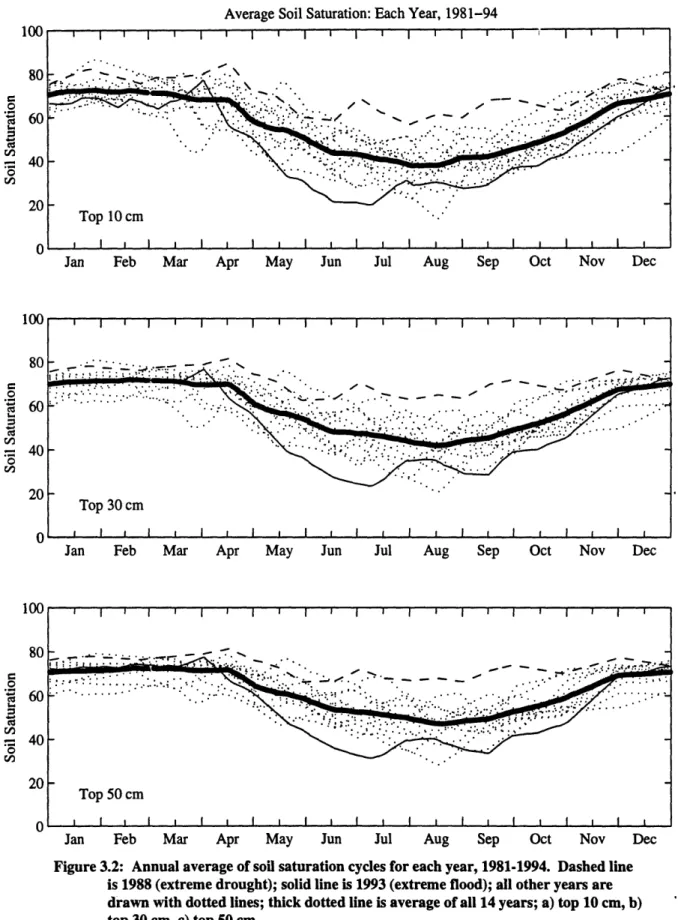
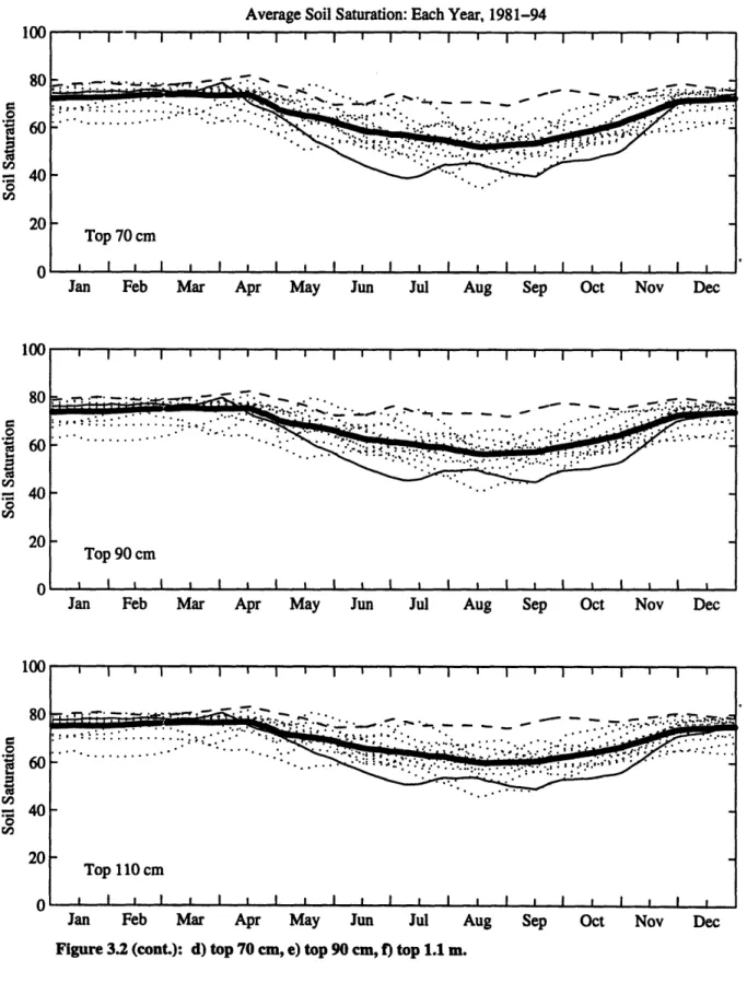
calculated by an appropriately weighted average of saturation within each 10 or 20 cm sample interval. Figures 3.2a-f show the average soil saturation for each of the 14 years for the top six surface layers, each highlighting 1988, a substantial drought year, and 1993, a substantial flood year. Figures 3.3a-d show seasonal average profiles of soil saturation, also highlighting 1988 and
1993. The summertime average (JJA) shows that during both of these extreme conditions, in the top meter of the profile 1988 is the driest of all the years and 1993 is the wettest of all the years. The effect of even the well-known drought of 1988 did not reach below this top meter of the soil: the soil between one and two meters was wetter than average during 1988. This is an indication that, in Illinois, effects of atmospheric phenomena do not reach below the top meter of the soil.' This is consistent with the fact that most of the state is covered with crops, which tend to have a rooting depth of close to one meter.
Average Soil Saturation: Each Year, 1981-94
Jan Feb Mar Apr May Jun Jul Aug Sep Oct Nov Dec
I 1 1 1 I I g I I ' I 11'
-
....
...
cTop 30 cm
I I I I i 1 i I1 I I I lI I i lI
Feb Mar Apr May Jun Jul Aug Sep Oct Nov Dec
Jan Feb Mar Apr May Jun Jul Aug Sep Oct Nov Dec Figure 3.2: Annual average of soil saturation cycles for each year, 1981-1994. Dashed line
is 1988 (extreme drought); solid line is 1993 (extreme flood); all other years are drawn with dotted lines; thick dotted line is average of all 14 years; a) top 10 cm, b) top 30 cm, c) top 50 cm. 100 80 40 20 0 100 80 Jan
Average Soil Saturation: Each Year, 1981-94 100 80 60 40 20 0 100 80 60 40 20 0 100 80 60 40 20 0
Jan Feb Mar Apr May Jun Jul Aug Sep Oct Nov Dec
Jan Feb Mar Apr May Jun Jul Aug Sep Oct Nov Dec Figure 3.2 (cont.): d) top 70 cm, e) top 90 cm, f) top 1.1 m.
MAM Soil Moisture Profile
S.
.. : : .. 2.4 . 0 . °··' c 0 50 100io
r 150 200 0 S50 S100 S150 200 50 100 15U 200. 50 100 150 200 0w o 0. 0. 0. 0. 0.2 0.4 0.6 0.8 Soil SaturationSON Soil Moisture Profile
B.
Daily Precipitation
Data
Measures of daily precipitation were available from the Illinois State Water Survey at 129 stations within the state. Their locations are shown in Figure 3.1. In Kunkel et al. (1990), data from these stations were bulked into 9 crop reporting zones: here, however, we have determined the state-wide average daily precipitation by averaging daily values at all 129 stations. This time series of the state-wide average daily rainfall was used in all the analyses discussed below. Figure
) 0.2 0.4 0.6 0.8
Soil Saturation
JJA Soil Moisture Profile
•~ ". .."".:.... .'."" .'.. _ .· .. :... . . :.... .. . • : 0 Figure I
i
t .. . . ....
IS
...
I IDJF Soil Moisture Profile
0.2 0.4 0.6 0.8 1 0 0.2 0.4 0.6 0.8
Soil Saturation Soil Saturation
3.3: Seasonal average soil saturation profiles: a) December-February (DJF), b)
March-May (MAM), c) June-August (JJA), d) September-November (SON). Left-most solid line is 1988 (extreme drought); right-Left-most solid line is 1993 (extreme flood); all other years are drawn with dotted lines; dashed line is average of all 14 years. · • ° I
...
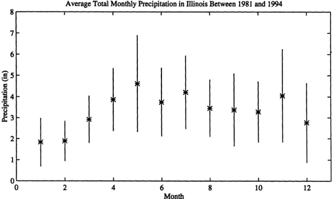
"' .e·· ··3.4 shows the average total monthly rainfall during the 14 years for which we have soil moisture observations (1981-1994).
Average Total Monthly Precipitation in Illinois Between 1981 and 1994
7- 6-5 5-0. 2-1 0 2 4 6 8 10 12 Month
Figure 3.4: Average total monthly precipitation over Illinois, 1981-1994. Stars indicate
means of the 14 years; lines extend to plus or minus one standard deviation.
C.
Results and Discussion: The Interplay Between Soil Saturation and
Subsequent Precipitation Throughout the Year
To relate this data analysis with the modeling discussed in the first chapter, we compared an initial soil condition to subsequent precipitation, much like a modeler would test for
precipitation sensitivity to soil water. For a given day, say April 1, we looked at the average soil saturation within the state for each of the available 14 years. We then calculated the total
precipitation in the subsequent 21 days for each of the 14 years, in this case, April 2 through April 23. Twenty-one days is time enough for the system to go through a few wetting and drying soil cycles, and a few convective storm cycles, so our results will be indicative not of a single weather event, but of a short climatic period. A linear regression was then performed on these two 14
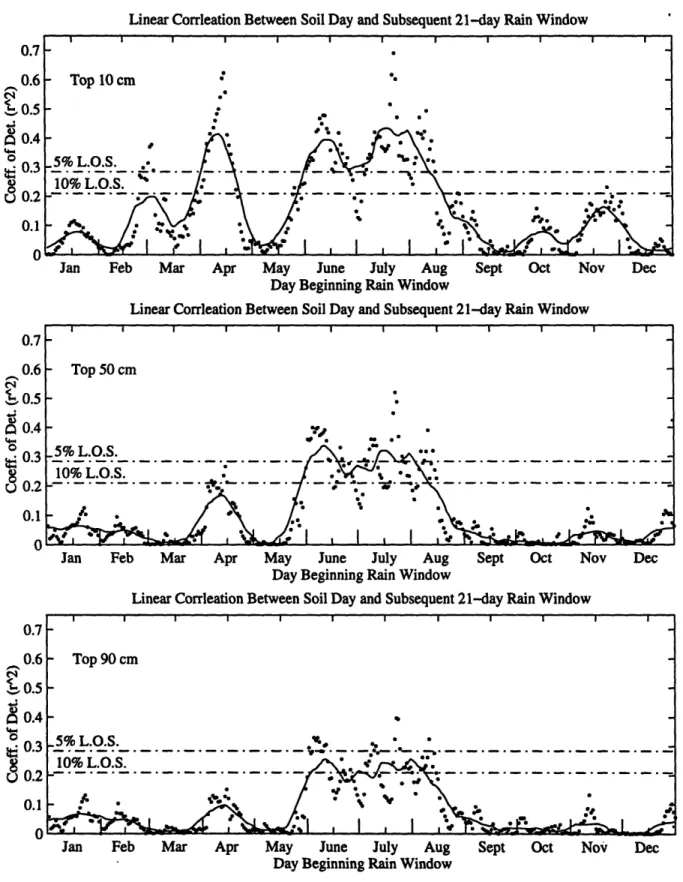
year series, and the coefficient of determination, r, was recorded as an indicator of the percentage of rainfall variability that can be explained by the soil water initial condition. This analysis was performed for all 365 days of the year. The dots in Figure 3.5 show that the ? values reach as high as 0.7 for the top 10 cm. Even after a 21 day smoothing, more than 40% of the variability in rainfall can be explained by a simple linear correlation between initial soil saturation and
subsequent rainfall. This correlation was damped at greater depths, but was still significant during the summer down to a depth of 90 cm.
The level of significance lines of Figure 3.5 are computed using an F-distribution for the r2. (The 5% level of significance line for an F distribution with 1 and 12 degrees of freedom in the numerator and denominator, respectively, is 4.75. This yields an r2 of 0.2836. The 10% line is at F(1,12) = 3.18, which yields an r2 of 0.2095. See Johnston (1984) for details.) These lines apply to the daily measurements, not to the smoothed lines. The significance lines for the smoothed data will be lower since the variability will go down as the inverse of the length of the averaging window. All Figures 3.5a-c show the daily ? is stronger during the summer than the rest of the year, though there is also a local peak during April, as well. At the shallower depths, the linear correlation stays above the 10% level of significance line from the end of May to early August, and for much of April. During the rest of the year, the correlation between soil moisture and subsequent precipitation is not significant. We find three possible explanations for these results showing that there is a significant linear relation between soil saturation and subsequent
Linear Corrleation Between Soil Day and Subsequent 21-day Rain Window
Jan Feb Mar Apr May June July Aug Sept Oct Nov Dec Day Beginning Rain Window
Linear Corrleation Between Soil Day and Subsequent 21-day Rain Window
Jan Febb Mar Apr May June July Aug Sept Oct Nov Dec Day Beginning Rain Window
Linear Corrleation Between Soil Day and Subsequent 21-day Rain Window
Jan Feb Mar Apr May June July Aug Sept Oct Nov Dec Day Beginning Rain Window
Figure 3.5: Linear correlation between Initial soil saturation and precipitation in the
subsequent 21 days for a) top 10 cm, b) top 50 cm, and c) top 90 cm. Solid line is
21-day moving average. Level of significance lines refer to the daily values (not the smoothed line). 0. 0. S0.0.. 0. 0. 4-0 4-0. 0. ' 0. 0. v