Biosphere-atmosphere interaction in a one-dimensional climate model of the tropics

(1)

Biosphere-Atmosphere

Interaction in a

One-Dimensional

Climate Model of the Tropics

by

Julie E. Kiang

Submitted to the Department

of Civil and Environmental

Engineering

in partial fulfillment of the requirements for the degree of

Master of Science in Civil and Environmental

Engineering

at the

MASSACHUSETTS

INSTITUTE

OF TECHNOLOGY

January

1999

[ Fe6YV1

ell/I

U) /9!Jj]

@

Massachusetts

Institute

of TecHnology 1999. All rights reserved.

Author...

.

DwaI/tment

of Civil and EnvironmeIitat'Engineering

January

15, 1999

Certified by ....

Elfatih A.B. Eltahir

Associate Professor

Thesis Supervisor

Accepted by

'~ ..~

"

.

Andrew J. Whittle

Chairman, Department

Committee on Graduate

Students

MASSACHUSETTS INSTITUTE

OF TECHNOLOGY

(2)

(3)

Biosphere-Atmosphere Interaction in a One-Dimensional

Climate Model of the Tropics

by

Julie E. Kiang

Submitted to the Department of Civil and Environmental Engineering

on January 15, 1999, in partial fulfillment of the

requirements for the degree of

Master of Science in Civil and Environmental Engineering

Abstract

In this study, we develop a one-dimensional model of the tropics which includes

two-way interaction between the biosphere and the atmosphere. The model integrates

a radiative-convective equlibrium model of the atmosphere, a land surface model

including plant growth and competition and a monsoon circulation model which

allows for the exchange of heat and moisture between the one-dimensional column

and its surroundings. The model is applied to two domains in West Africa to test the

sensitivity of the system's equilibrium to perturbations to initial vegetation.

In the coastal domain, the model simulates a stable forest equilibrium. The

equilibrium climate and vegetation show reasonable similarity to observations for

the same region. The same equilibrium is reached in both our control simulation

and our experimental simulation, in which deforestation is simulated by initializing

the model with grassland. Modifications to parameters of the empirical monsoon

circulation model show that the climate and vegetation in our model domain are

sensitive to the strength of the monsoon circulation and also to climatic conditions

in adjacent regions. In particular, changes in the monsoon which allowed hot and

dry air to penetrate into the model domain from the north strongly affected the

equilibrium climate and vegetation. These sensitivity studies indicated that the

existence of multiple equilibria in the biosphere-atmosphere system depends not only

on the magnitude of the vegetation-induced climate perturbation, but also on whether

or not the perturbation extends across a threshold controlling competition between

trees and grasses.

In the inland domain, the model simulates a stable grassland equilibrium in both

the control simulation and an afforestation experiment. While vegetation conditions

in the inland domain strongly affected the energy balance, primarily through c~anges

in surface albedo, they had little effect on precipitation and moisture availability.

Thesis Supervisor: Elfatih A.B. Eltahir

(4)

Acknowledgments

This research was funded in part by NASA Agreement NAGW-5201. In addition,

I was fortunate to be supported by an NSF Graduate Research Fellowship, an NSF

Traineeship in the Hydrological Sciences, a Ralph M. Parsons Fellowship and a Global

Clirnate Modelling Initiative Fellowship. I am grateful to all the organizations which

provided financial support for this research.

Some components of the model developed in this study were provided courtesy of

Nilton Renno, now at the University of Arizona, and Jonathan Foley and his group

at the University of Wisconsin, Madison. Their advice and patience while I was

farniliarizing myself with their models is much appreciated. Dave Pollard at NCAR

was also helpful during this process.

NIy research advisor, Elfatih Eltahir, continually challenged me to incorporate

new ideas into my work and to strive to be as comprehensive as possible during all

phases of the research. My thanks also to the members of my research group, whose

friendship, support, and sharing of knowledge were invaluable to the completion of

this thesis. Special thanks to Guiling Wang, for many hours of discussion on modeling

techniques and simulation results, to Kirsten Findell, for her unflagging support, and

to Jeremy Pal, for help during various stages of this work.

NIy experience at MIT would have been far less enjoyable without the close

friendships which I've developed over the past few years. Thanks to all of you for

rnaking the East Coast a fun place to live and work, especially Sue and Erica, for

helping me to forge a home in the big city, Karen P., for helping to bridge the past

and the present, and Jon, for new adventures. Thanks also to my friends and family

back home in California and scattered around the world, whose silent cheering have

(5)

Introduction

23

2 Biosphere - Atmosphere Interactions

29

2.1 Climatic controls on vegetation 29

2.1.1 Theory... 29

2.1.2 Previous modeling studies 31

2.2 Land surface / vegetation controls on climate 33

2.2.1 Theory... 33

2.2.2 Observational studies . 38

2.3 Two-way feedbacks 42

2.3.1 Theory... 42

2.4 Monsoon circulations and their sensitivity to land surface conditions. 45

2.4.1 Theory of monsoon circulations . . . 45

2.4.2 Modeling studies of monsoon - vegetation interaction 49

3 Climatology and Ecology of West Africa

51

3.1 Climate of West Africa . . 51

3.2 Vegetation of West Africa 56

3.2.1 Tropical forest. . . 63

3.2.2 Savanna and grassland 64

(6)

4

Model Description

67

4.1 Atmospheric Component: Radiative-Convective Equilibrium Model 68

4.2 Land Surface Component: Integrated Biosphere Simulator (IBIS) 71

4.3 lVIonsoon Circulation Model 80

4.4 Coupled Model . . . 88

5

Coastal Domain: Experimental Simulations

89

5.1 Control Simulations 91

5.1.1 Control simulation: Fixed circulation 91

5.1.2 Control simulation: Interactive circulation 100

5.1.3 Sensitivity to mixed layer depth . . . 107

5.1.4 Sensitivity to modifications in land surface model 113

5.2 Deforestation Experiments: Fixed Circulation Case 115

5.2.1 Static vegetation simulations. . 116

5.2.2 Dynamic vegetation simulations 117

5.3 Deforestation experiments: Interactive Circulation Case. 125

5.4 Sensitivity of Results to Slope of Empirical Flux Relationships 126

5.5 Sensitivity of Results to Properties of the Advected Air 149

5.5.1 Static Vegetation Simulations . 151

6 Inland Domain: Experimental Simulations

165

6.1 Control Simulations. . . 166

6.1.1 Control Simulation: Fixed Circulation 167

6.1.2 Control Simulation: Interactive Circulation. 178

6.2 Afforestation Experiments: Fixed Circulation Case 184

(7)

6.2.2 Dynamic vegetation simulations .

6.3 Afforestation Experiments: Interactive Circulation Case .

6.3.1 Static Vegetation Simulations .

6.3.2 Dynamic vegetation simulations

6.4 Sensitivity of Results to Slope of Empirical Flux Relationship

6.5 Sensitivity of Results to Properties of the Advected Air

7 Conclusion

7.1 Further Research

A Biomass Initialization

A.l Coastal domain simulations

A.2 Inland domain simulations .

185

190

193

201 203

205

209

210

211

(8)

(9)

List of Figures

1-1 Components of the surface water balance.

1-2 Components of the surface energy balance.

24

25

2-1 Characteristics of vegetation which affect the surface energy balance. 35

2-2 (a) Summer (June, July, August) winds over West Africa. (b) Winter

(December, January, February) winds over West Africa. . . .. 47

2-3 A strong gradient in boundary layer entropy is associated with a strong

monsoon circulation. Conversely, a weak gradient in boundary layer

entropy is associated with a weak monsoon circulation. . . .. 48

3-1 The upper panel shows the monthly precipitation [mm/day] at 3

stations in West Africa. (Source: Rumney, 1968) The lower panel

shows the mean annual precipitation [mm/day] in West Africa as given

by the NCEP reanalysis clilnatology (1982-1994). ., . . . .. 54

3-2 Evapotranspiration [mm/day], NCEP reanalysis climatology

(1982-1994). ... . . . .. 55

3-3 Specific humidity [kg/kg], NCEP reanalysis climatology (1982-1994). 56

3-4 The upper panel shows the average monthly temperature [K] at 3

stations in West Africa. (Source: Rumney, 1968) The lower panel

shows the mean annual temperature [K] in West Africa as given by the

NCEP reanalysis climatology (1982-1994). . . .. 57

3-5 Shortwave radiative flux [W

/m

2], NCEP reanalysis climatology

(10)

3-6 Net shortwave radiation [W

1m2],

NCEP reanalysis climatology

(1982-1994). . . .. 59

3-7 Net longwave radiation

[W

1m

2], NCEP reanalysis climatology

(1982-1994). 60

3-8 Net all wave radiation

[W

1m

2

], NCEP reanalysis climatology (1982-1994). 61

3-9 Boundary layer entropy

[JIkg/K],

NCEP reanalysis climatology

(1982-1994). . . .. 62

4-1

An

illustration of our model's interaction with its surroundings. How

does this interaction and characteristics of the land surface affect the

vegetation-climate equilibrium? . . . .. 68

4-2 The function, qgfac, as a function of near surface soil saturation before

and after our modification. The modified curve is the expected value

of qgfac as a function of the expected value of the near surface soil

saturation. . . 79

4-3 The solid box shows the model domain, the dotted box shows the

associated ocean region used in developing the empirical Inonsoon

circulation model. (a) Coastal domain (b) Inland domain. . . .. 84

4-4 Coastal domain: Mass fluxes of air into the domain vs. entropy

difference between land and ocean. (a) Flux from south (across 5N).

(b) Flux from north (across ION). . . .. 85

4-5 Inland domain: Mass fluxes of air into the domain vs. entropy

difference between land and ocean. (a) Flux from south (across ION).

(b) Flux from north (across 15N). . . .. 86

4-6 Coastal domain: correlation between mass flux of air and differences in

specific humidity and temperature. (a) Specific Humidity - Flux from

south (across 5N). (b) Specific Humidity - Flux from north (across

ION). (c) Temperature - Flux from south (across 5N). (d) Temperature

(11)

5-1 Coastal domain, fixed circulation control simulation. The upper panel

shows the LAI, which is stable throughout the run. The lower panel

shows the biomass, which has not yet stabilized. . . .. 93

5-2 Coastal domain: NCEP reanalysis climatology (1982-1994), seasonal

cycle of climate. (a) Temperature (b) Precipitation (c) Specific

humidity (d) Total evapotranspiration (e) Boundary layer entropy (f)

Runoff. . . .. 96

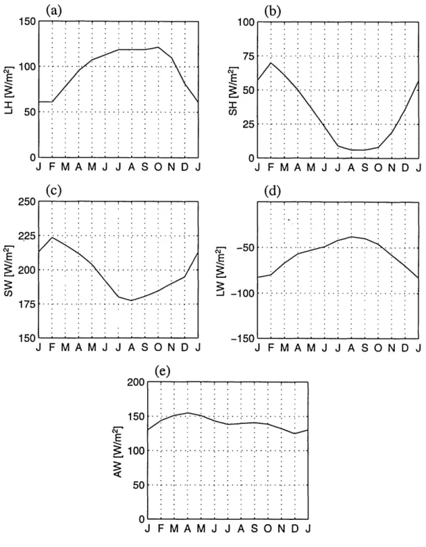
5-3 Coastal domain: NCEP reanalysis climatology (1982-1994),

land-atmosphere energy exchange. (a) Latent heat flux (b) Sensible heat

flux (c) Net shortwave radiative flux (d) Net longwave radiative flux

(e) Net allwave radiative flux 97

5-4 Coastal domain:

N CEP reanalysis climatology (1982-1994), atmospheric soundings. (a)

Absolute temperature (b) Potential temperature (c) Specific humidity

(d) Relative humidity. . . .. 98

5-5 Coastal domain: fixed circulation control simulation, seasonal cycle

of simulated climate. (a) Temperature (b) Precipitation (c) Specific

Runoff. . . .. 101

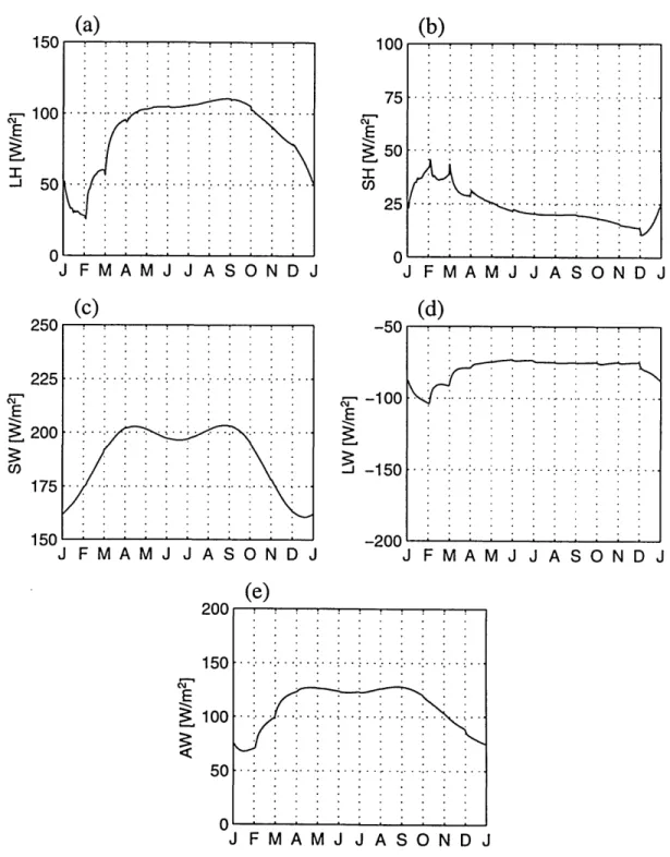
5-6 Coastal domain: fixed circulation control simulation, land-atmosphere

energy exchange. (a) Latent heat flux (b) Sensible heat flux (c) Net

shortwave radiative flux (d) Net longwave radiative flux (e) Net allwave

radiative flux . . . .. 102

5-7 Coastal domain: fixed circulation control simulation, monsoon

circulation. (a) Heat advection (b) Moisture advection (c) Lowest level

wind across southern boundary (d) Lowest level wind across northern

boundary (e) Entropy difference between model domain and ocean

(12)

5-8 Coastal domain: fixed circulation control simulation, atmospheric

soundings. (a) Absolute temperature (b) Potential temperature (c)

Specific humidity (d) Relative humidity 104

5-9 Coastal domain, fixed circulation control simulation. The upper panel

shows the LAI, which is stable throughout the run. The lower panel

shows the biomass, which has not yet stabilized. . . .. 108

5-10 Coastal domain: interactive circulation control simulation, seasonal

cycle of simulated climate. (a) Temperature (b) Precipitation (c)

Specific humidity (d) Total evapotranspiration (e) Boundary layer

entropy (f) Runoff . . . .. 109

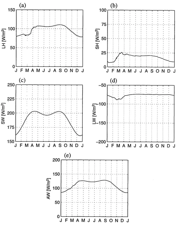
5-11 Coastal domain: interactive circulation control simulation,

flux (c) Net shortwave radiative flux (d) Net-Iongwave radiative flux

5-12 Coastal domain: interactive circulation control simulation, monsoon

region (f) Precipitable water . . . .. III

5-13 Coastal domain: interactive circulation

control simulation, atmospheric soundings. (a) Absolute temperature

(b) Potential temperature (c) Specific humidity (d) Relative humidity 112

5-14 Coastal domain: fixed circulation fixed grass simulation, seasonal cycle

Runoff. . . 118

5-15 Coastal domain: fixed circulation fixed grass simulation,

(13)

5-16 Coastal domain: fixed circulation fixed grass simulation, monsoon

region (f) Precipitable water . . . .. 120

5-17 Coastal domain: fixed circulation fixed grass simulation, atmospheric

5-18 Coastal domain, fixed circulation simulations. Vegetation is initialized

as either deciduous forest or grassland. The equilibrium vegetation

LAI is the same in either case. . . .. 123

5-19 Coastal domain, fixed circulation simulations. The equilibrium

biomass approaches the same value whether the simulation is initialized

as deciduous forest or grassland. . . .. 124

5-20 Coastal domain: interactive circulation fixed grass simulation, seasonal

cycle of simulated climate. (a) Temperature (b) Precipitation (c)

Specific humidity (d) Total evapotranspiration (e) Boundary layer

entropy (f) Runoff ... . . . .. 127

5-21 Coastal domain: interactive circulation fixed grass simulation,

(e) Net allwave radiative flux . . . .. 128

monsoon circulation. (a) Heat advection (b) Moisture advection

(c) Lowest level wind across southern boundary (d) Lowest level

wind across northern boundary (e) Entropy difference between model

domain and ocean region (f) Precipitable water . . . .. 129

atmospheric soundings. (a) Absolute temperature (b) Potential

(14)

5-24 Coastal domain: Whether the initial vegetation is forest or grassland,

the model simulates the same equilibrium vegetation and climate

(evergreen forest), here represented by the leaf area index (LAI). . .. 131

5-25 Coastal domain: The equilibrium biomass approaches the same value

whether the simulation is initialized as forest or grassland. . . .. 132

5-26 Coastal domain: SouthX2, seasonal cycle of simulated climate.

(a) Temperature (b) Precipitation (c) Specific humidity (d) Total

evapotranspiration (e) Boundary layer entropy (f) Runoff 135

5-27 Coastal domain: SouthX2: Land-atmosphere energy exchange (a)

Latent heat flux (b) Sensible heat flux (c) Net shortwave radiative

flux (d) Net longwave radiative flux (e) Net all wave radiative flux .. 136

5-28 Coastal domain: SouthX2, Monsoon circulation. (a) Heat advection

(b) Moisture advection (c) Lowest level wind across southern boundary

(d) Lowest level wind across northern boundary (e) Entropy difference

between model domain and ocean region (f) Precipitable water. . .. 137

5-29 Coastal domain: NorthX2, seasonal cycle of simulated climate.

5-30 Coastal Domain: NorthX2, Land-atmosphere energy exchange. (a)

Latent heat flux (b) Sensible heat flux (c) Net shortwave radiative flux

(d) Net longwave radiative flux (e) Net allwave radiative flux ... 139

5-31 Coastal domain: NorthX2, Monsoon circulation. (a) Heat advection

5-32 Coastal domain: SouthX2 with fixed grass, seasonal cycle of simulated

climate. (a) Temperature (b) Precipitation (c) Specific humidity (d)

(15)

5-33 Coastal domain: SouthX2 with fixed grass, land-atmosphere energy

exchange. (a) Latent heat flux (b) Sensible heat flux (c) Net shortwave

radiative flux (d) Net longwave radiative flux (e) Net allwave radiative

flux. . . .. 144

5-34 Coastal domain: SouthX2 with fixed grass, monsoon circulation. (a)

Heat advection (b) Moisture advection (c) Lowest level wind across

southern boundary (d) Lowest level wind across northern boundary

(e) Entropy difference between model domain and ocean region (f)

Precipitable water. . . .. 145

5-35 Coastal domain: NorthX2 with fixed grass, seasonal cycle of simulated

Total evapotranspiration (e) Boundary layer entropy (f) Runoff ... 146

5-36 Coastal domain: NorthX2 with fixed grass, land-atmosphere energy

~xchange. (a) Latent heat flux (b) Sensible heat flux (c) Net shortwave

radiative flux (d) Net longwave radiative flux (e) Net allwave radiative

flux. . . .. 147

5-37 Coastal domain: NorthX2 with fixed grass, monsoon circulation. (a)

Heat advection (b) Moisture advection (c) Lowest level wind across

southern boundary (d) Lowest level wind across northern boundary

(e) Entropy difference between model domain and ocean region (f)

Precipitable water. . . .. 148

5-38 Coastal domain: Advect15, seasonal cycle of simulated climate.

5-39 Coastal domain: Advect15, land-atmosphere energy exchange. (a)

Latent heat flux (b) Sensible heat flux (c) Net shortwave radiative

(16)

5-40 Coastal domain: Advect15, monsoon circulation. (a) Heat advection

5-41 Coastal domain: Advect15, atmospheric soundings. (a) Absolute

temperature (b) Potential temperature (c) Specific humidity (d)

Relative humidity 155

5-42 Coastal domain: Advect15 with grass initialization, seasonal cycle

Runoff. . . .. 156

5-43 Coastal domain: Advect15 with grass initialization, land-atmosphere

shortwave radiative flux (d) Net longwave radiative flux (e) Net allwave

radiative flux . . . .. 157

5-44 Coastal domain: Advect15 with grass initialization, monsoon

circulation. (a) Heat advection (b) lVIoisture advection (c) Lowest level

5-45 Coastal domain: Advect15 with grass initialization, atmospheric

5-46 Coastal domain: Advect15, the equilibrium vegetation, here described

by LAI, is different when the simulation is initialized with forest versus

grassland. . . .. 162

5-47 Coastal domain: Advect15, the equilibrium vegetation, here described

by biomass, is different when the simulation is initialized with forest

(17)

6-1 Inland domain: Fixed circulation simulations. At equilibrium,

grassland is dominant in terms of both LAI and biomass for the control

simulation, initialized with grassland. . . .. 168

6-2 Inland domain: NCEP reanalysis climatology (1982-1994), seasonal

cycle of climate. (a) Temperature (b) Precipitation (c) Specific

Runoff. . . .. 169

6-3 Inland domain: N CEP reanalysis climatology (1982-1994),

6-4 Inland domain:

NCEP reanalysis climatology (1982-1994), atmospheric soundings. (a)

Absolute temperature (b) Potential temperature (c) Specific humidity

(d) Relative humidity 171

6-5 Inland domain: fixed circulation control simulation, mean annual

Total evapotranspiration (e) Boundary layer entropy (f) Runoff . .. 174

6-6 Inland domain: fixed circulation control simulation, land-atmosphere

shortwave radiative flux (d) Net longwave radiative flux (e) Net all wave

radiative flux .. . . .. 175

6-7 Inland domain: fixed circulation control simulation, monsoon

6-8 Inland domain: fixed circulation control simulation, atmospheric

(18)

6-9 Inland domain: Interactive circulation simulations. At equilibrium,

grassland is dominant in terms of both LAI and biomass for the control

simulation, initialized with grassland. . . .. 179

6-10 Inland domain: interactive circulation control simulation, mean annual

Total evapotranspiration (e) Boundary layer entropy (f) Runoff . .. 180

6-11 Inland domain: interactive circulation control simulation,

(e) Net all wave radiative flux 181

6-12 Inland domain: interactive circulation control simulation, monsoon

6-13 Inland domain: interactive circulation control simulation, atmospheric

6-14 Inland domain: fixed circulation control simulation, mean annual

climate, fixed deciduous forest. (a) Temperature (b) Precipitation

(c) Specific humidity (d) Total evapotranspiration (e) Boundary layer

entropy (f) Runoff . . . .. 186

6-15 Inland domain: fixed circulation control simulation, land-atmosphere

energy exchange, fixed deciduous forest. (a) Latent heat flux (b)

Sensible heat flux (c) Net shortwave radiative flux (d) Net longwave

(19)

6-16 Inland domain: fixed circulation control simulation, monsoon

circulation, fixed deciduous forest. (a) Heat advection (b) Moisture

advection (c) Lowest level wind across southern boundary (d) Lowest

level wind across northern boundary (e) Entropy difference between

model domain and ocean region (f) Precipitable water. . . .. 188

6-17 Inland domain: fixed circulation control simulation, atmospheric

soundings, fixed deciduous forest. (a) Absolute temperature (b)

Potential temperature (c) Specific humidity (d) Relative humidity .. 189

grassland is dominant with the same LAI, regardless of the initial

vegetation conditions. . . .. 191

grassland is dominant with the same biomass, regardless of the initial

vegetation conditions. . . .. 192

6-20 Inland domain: interactive circulation control simulation, mean annual

climate, fixed deciduous forest. (a) Temperature (b) Precipitation

(c) Specific humidity (d) Total evapotranspiration (e) Boundary layer

entropy (f) Runoff ... . . 194

6-21 Inland domain: interactive circulation control simulation,

land-atmosphere energy exchange, fixed deciduous forest. (a) Latent heat

flux (b) Sensible heat flux (c) Net shortwave radiative flux (d) Net

longwave radiative flux (e) Net allwave radiative flux . . . .. 195

6-22 Inland domain: interactive circulation control simulation, monsoon

circulation, fixed deciduous forest. (a) Heat advection (b) Moisture

advection (c) Lowest level wind across southern boundary (d) Lowest

level wind across northern boundary (e) Entropy difference between

model domain and ocean region (f) Precipitable water. . . .. 196

6-23 Inland domain: interactive circulation control simulation, atmospheric

soundings, fixed deciduous forest. (a) Absolute temperature (b)

(20)

grassland is dominant with the same LAI, regardless of the initial

vegetation conditions.. . . 198

grassland is dominant with the same biomass, regardless of the initial

vegetation conditions. . . 199

A-I Coastal domain, fixed circulation simulation, deciduous forest

initialization. Both the LAI (upper panel) and the biomass (lower

panel) show that evergreen forest is beginning to grow at the end of

this simulation, in which the biomass is initialized at 15 kg-C/m2• •. 212

A-2 Coastal domain, fixed circulation simulation, deciduous forest

initialization. Both the LAI (upper panel) and the biomass (lower

panel) show that the deciduous forest is giving way to evergreen forest

at the end of this simulation, in which the biomass is initialized at 15

kg-C

1m

2

• • • • • • • • • • • • • • • • . . . • • . . . • • . . • .. 213

A-3 Inland domain, interactive circulation simulation, deciduous forest

initialization. The upper panel shows the sudden drop in LAI at the

beginning of the simulation due to the negative NPP. The lower panel

(21)

List of Tables

2.1 Results from Modeling Studies of Amazonian Deforestation. . . . .. 39

3.1 Typical values of NPP, biomass and LAI for tropical ecosystems. . .. 66

4.1 IBIS standalone run with climatological forcing. Location: 6E, 8N .. 75

4.2 IBIS standalone run for fixed evergreen forest with and without

modifications for subgrid variability in interception storage and bare

soil evaporation. . . .. 76

4.3 IBIS standalone run for fixed grassland with and without modifications

for subgrid variability in interception storage and bare soil evaporation. 76

5.1 Coastal Domain Control Runs - Simulated Mean Annual Climate with

Comparison to NCEP Climatology . . . .. 94

5.2 Coastal Domain: Sensitivity to Mixed Layer Depth 113

5.3 Fixed evergreen forest with and without modifications for subgrid

variability in interception storage and bare soil evaporation. ... 114

5.4 Fixed grassland with and without modifications for subgrid variability

in interception storage and bare soil evaporation. 115

(22)

5.6 Coastal Domain: Modelled Forest vs. Grassland, Compared to

Previous Modeling Studies of Amazonian Deforestation. While strict

comparisons should not be made due to the different locations of these

studies, we can note that in almost all cases the sign of the changes

in the listed variables are the same in our experiments and in the

Amazonian deforestation experiments. 122

5.7 Coastal Domain: Sensitivity of forested domain to the slope of the

empirical flux relationships. 134

5.8 Coastal Domain: Modelled Forest vs. Grassland, with modified

monsoon circulation (Experiments SouthX2 and South+2 . . . .. 141

5.9 Coastal Domain: Modelled Forest vs. Grassland, with modified

monsoon circulation (Experiments NorthX2 and North+2 . 142

5.10 Coastal Domain: Summary of equilibrium vegetation. . . . 149

5.11 Coastal Domain: Modelled Forest vs. Grassland, with modified profile

of advected air (Experiment Advect15) . . . .. 160

6.1 Inland Domain Control Run - Simulated Mean Annual Climate with

Comparison to NCEP Climatology . . . 173

6.2 Inland Domain: Modelled Forest vs. Grassland. 185

6.3 Inland Domain: Modelled Forest vs. Grassland, with modified

monsoon circulation. . . 200

6.4 Inland Domain: Modelled Forest vs. Grassland, with modified

horizontal air fluxes and advection. . . 201

6.5 Inland Domain: Summary of equilibrium vegetation. 202

7.1 Coastal Domain: Summary of equilibrium vegetation.

7.2 Inland Domain: Summary of equilibrium vegetation.

207 208

(23)

Chapter

1 Introduction

Since prehistoric times, humans have been altering the earth's environment to make

it more hospita:ble for daily life, to obtain necessary food and shelter, and rnore

recently, to extract economic gain from its vast resources. Over the past few

centuries, and particularly within the previous few decades, rapid population growth

and technological advances have encouraged swifter and more dramatic changes to

natural conditions. These human-wrought changes to the earth have become the

subject of great controversy, and to some, cause for great alarm. In particular,

numerous studies have suggested that rapid deforestation in the tropics may be

significantly impacting both regional and global climate. In the face of this concern, a

thorough understanding of the interplay between land surface conditions and climate

is warranted, as it can allow us to better manage the earth's resources for future as

well as current generations.

The earth's vegetation contributes significantly to the global carbon cycle,

acting as a storage reservoir which allows active exchange of carbon with the

atmosphere. Vegetation thus has a significant influence on atmospheric carbon

dioxide concentrations worldwide. Carbon dioxide is an important greenhouse

gas, and changes in vegetation cover affecting carbon dioxide concentrations can

influence climate worldwide. While vegetation's role in the carbon cycle has

received widespread media coverage, vegetation also affects local or regional climate

(24)

Atmosphere

Land Surface evapotranspiration

~ runoff

---I

drainage

Figure 1-1: Components of the surface water balance.

atmosphere. In fact, these fluxes may have a greater influence on climate than changes

in atmospheric carbon dioxide concentrations, especially at a local or regional scale.

The effects of vegetation on the fluxes of water and energy between the biosphere and

the atmosphere are the focus of this study. Figure 1-1 and Figure 1-2 depict the fluxes

comprising the water balance and the energy balance at the biosphere - atmosphere

interface. Vegetation affects the strength of these fluxes and the partitioning between

them and in this way influences atmospheric and climatic conditions. In turn, local

climate affects the types of vegetation which exist in a particular location as different

plants have different tolerances for heat, moisture, and light availability, and different

strategies for competition when these resources are scarce. This two-way interaction

between vegetation and climate determines the equilibrium state of vegetation and

climate for a given region.

Speculations on the importance of interactions between the land surface and

the atmosphere began centuries ago. It is said that Christopher Columbus noted

(25)

downwards1longwave

A

tin os

ph

ere

radiation

~~d S;rf;c~- -

t

';p;;"dsloyw-;;;e ...diation

latent heat flux

reflected solar radiation

Figure 1-2: Components of the surface energy balance.

the originally high rainfall to the existence of forests on the islands (Meher-Homji

1988). More recently, scientific research has led to improved understanding of

the role of vegetation in determining atmospheric conditions. Significant research

activity has been undertaken to predict the response of global and regional climate to

deforestation. These studies have shown that the control plants exert over moisture

and heat fluxes between the land surface and the atmosphere can have significant

impacts on atmospheric conditions. Numerous modeling studies of Amazonian

deforestation, for example, have consistently shown that large scale deforestation

results in a warmer and drier climate in the deforested tropical region (e.g., Lean and

Warrilow, 1989; Shukla et aI, 1990; Eltahir and Bras, 1994; Sud et aI, 1996). However,

all of these studies have considered only a one way interaction between vegetation

and the climate system. Each of these studies treats vegetation as a static property

of the land surface, examining the differences between climate simulated when either

(26)

into forests, or vice-versa, despite climatic conditions which may favor one dominant

vegetation type or the other.

In this study, we address this problem by developing a one-dimensional climate

model which allows two way interaction between the biosphere's vegetation and the

overlying atmosphere. Plant life responds to changes in climatic conditions, which

are in turn influenced by vegetation conditions at the land surface. These changes in

climatic conditions can then further influence vegetation at the land surface, and so

on in a potential feedback loop. Whether or not inclusion of these two-way feedbacks

is important in determining the final equilibrium between vegetation and climate is

the subject of this study. If the two-way interaction is indeed important, different

initial conditions may result in different equilibrium states. Our model is used to

explore the response of the system to perturbations to vegetation at the land surface

(e.g., deforestation). Our experiments investigate the possibility of multiple equilibria

between vegetation and climate when perturbations to the system are made. Rather

than being a predictive tool, our model is intended to elucidate the processes and the

constraints which may encourage or inhibit the development of multiple equilibria.

A one-dimensional model was selected for its simplicity and for its ability to isolate

local effects from the effects of large scale circulations. The one-dimensional column

does, however, have limited interaction with its surroundings. An empirical model,

based upon theories of monsoon circulations, is developed to describe the exchange

of heat and moisture between the single column and surrounding regions.

The model describes the atmosphere as a one-dimensional column of air whose

state is determined by the interplay between radiative forcing, convection, boundary

conditions at the land surface, and heat and moisture transport arising from the

simulated monsoon circulation.

It

is suitable for use in tropical areas where the

climatic regime is dominated by convection rather than baroclinic frontal systems.

Such a condition is characteristic of the tropics, and to some extent, summer

in the mid-latitudes. In this study, we confine our work to the tropics, and in

particular, West Africa, where the zonal symmetry and clear circulation patterns

(27)

the surroundings.

Following this introduction, Chapter 2 provides background on the modes of

interaction between the biosphere and the atmosphere and briefly reviews previous

studies on the subject. Chapter 3 outlines some of the important climatological

and vegetal characteristics of the tropics, with particular attention to West Africa.

Chapter 4 describes our biosphere-atmosphere model, including each of the model's

subcomponents. Chapter 5 and Chapter 6 describe the setup of the experimental

runs and detail the results of the experiments conducted in two dOlnains, one along

the coast of West Africa, and one further inland. Finally, Chapter 7 summarizes the

(28)

(29)

Chapter 2 Biosphere - Atmosphere

Interactions

This chapter provides a discussion of theories of biosphere-atmosphere interaction as

well as an overview of previous modeling work dealing with biosphere-atmosphere

interactions. The effects of atmospheric conditions on vegetation at the land surface

are described, along with the role vegetation plays in affecting the atmosphere and

climate.

This two-way interaction creates the possibility of complicated feedbacks

between the biosphere and the atmosphere. The chapter concludes with a discussion

of these feedbacks and the potential impacts of land surface changes on monsoon

circulations.

2.1 Climatic controls on vegetation

2.1.1 Theory

Global maps of vegetation and climate show a marked correlation between vegetation

type and climate.

Similar vegetation is found in areas which experience similar

climatic regimes. This is not surprising, as plant growth and survival are dependent

upon many factors which are related to climate.

These factors include (Crawley

(30)

• Temperature maxima, minima and averages (daily and annual)

• Temperature ranges (daily and annual)

• Water availability and atmospheric humidity

• Light intensity

• Length of day

• Length of growing season

*

Soil type and depth

*

Availability of nutrients

*

Mechanical factors (e.g., the frequency of fire and wind damage and the amount

of grazing by animals)

Climate has a direct effect on the first six of these factors, and indirectly affects the

remaining three. Combinations of these factors produce environments in which some

plants and not others are able to survive.

While a particular plant may be able to survive in a wide range of climatic

conditions, the ability of a plant to thrive in a particular climate is influenced not

only by its absolute tolerances to various climatic variables, but also by its ability to

compete successfully against other plants vying for the same resources. Laboratory

experiments have shown that a plant's "physiological optimum" , the conditions under

which it is able to maximize growth when there is no competition from other plants,

is rarely the same as a plant's "ecological optimum", the conditions under which it is

able to maximize growth in the face of competition from other plants (Crawley 1986a).

In nature, plants are found where local conditions match their ecological optimum.

Typically, a plant is capable of existing in a far greater range of environments than it

is actually found to exist in nature, and is limited to the smaller observed range by

competition from other plant types.

Some important considerations in assessing the competitiveness of a plant species

(31)

• Ability to access resources (light, water, nutrients, soil/space)

• Need for these resources

• Growth and mortality rates

• Differences in seedling needs and established plant needs

The competitiveness of different tropical plant types in various environments are

discussed further in Chapter 3.

2.1.2 Previous modeling studies

Existing models which simulate the response of vegetation to climate have ranged from

simple models which predict global vegetation patterns, to models including detailed

descriptions of individual plants. Two categories of these models are described briefly

below.

Equilibrium vegetation models.

These types of models predict the equilibrium

vegetation for a region given the local climatology. They are typically used at large

scales. For example, this type of model is suitable for predicting vegetation cover using

the climate produced by a GCM. Because of the large scale at which these models are

applied, individual plants and plant species are not modeled. Rather, groupings

of plants which share similar climate tolerances, growth and mortality patterns,

and physical attributes are lumped together in what are often referred to as plant

functional types (Smith et al. 1993). Examples of common plant functional types for

the tropics are tropical evergreen trees, tropical raingreen (drought deciduous) trees,

C3 grasses and C4 grasses (Foley et al. 1996).

The simplest equilibrium vegetation models are based on correlations between

observed global patterns of vegetation and climate. These models often describe

vegetation as ecosystems such as tropical forest or tropical savanna, foregoing the use

of plant functional types in favor of an even more general description (Prentice et al.

(32)

Other equilibrium vegetation models are more mechanistic. For example, the

BlOME model (Prentice et al. 1992) determines equilibrium vegetation by first

determining what plant functional types can be expected to be able to survive in

a particular climatic regime. This is accomplished by defining physiological limits, or

tolerances, of quantities such as maximum and minimum temperature and moisture

availability for each plant functional type. After determining which plant functional

types could reasonably be expected to survive in a location, competition between the

plant functional types is treated indirectly by use of a dominance hierarchy. Certain

plant functional types will be excluded from a location by the presence of other plant

functional types which are known to compete more successfully for necessary resources

(Claussen 1997).

While equilibrium vegetation models have been used to model observed global

vegetation patterns, they are designed to predict equilibrium vegetation and are thus

unable to model the transient behavior of vegetation (Prentice et al. 1993). However,

in considering interactions between vegetation and climate, the transient behavior

may be quite important, especially if climatic change outpaces the response time of

vegetation. Interactions between vegetation and the climate may preclude transitions

from one state to another, thereby influencing the equilibrium state of the system.

Forest stand models/gap models.

This class of models provides representation

of individual trees and has been used to model the successional behavior of small

forest patches. The height, diameter, and other characteristics of individual trees

can be predicted. However, these models are suited for scales on the order of

1000 m2 _(Prentice _{et al. 1993), much smaller than is practical} _{for climate modeling.}

While useful in forestry, the detailed description of individual trees is not suited for

large scales, where the overall canopy structure is a more suitable descriptor of the

vegetation.

For integration with climate modeling, there is clearly a need for models which are

intermediate in complexity between the two classes of models described above. The

(33)

models which explicitly represents competition between plants in response to weather

conditions experienced during a particular year, but at a scale which is appropriate for

use in modeling regional climate. The level of detail in the description of vegetation

is similar to that of Surface- Vegetation-Atmosphere Transfer (SVAT) schemes such as

the Biosphere-Atmosphere Transfer Scheme (BATS) (Dickinson et al. 1986) and the

Simple Biosphere Model (SiB) (Sellers et al. 1986). Like SVAT's, IBIS is designed to

provide an atmospheric model with surface energy and moisture fluxes. IBIS is used

as the land surface component of our one-dimensional climate model, and is described

more fully in Chapter 4.

2.2 Land surface / vegetation

controls on climate

2.2.1 Theory

Linkages between the land surface and the atmosphere are evident when one considers

both the water and the energy balance at the land surface. Vegetation affects the

exchange of both heat and moisture between the land surface and the atmosphere,

and can thus play an important role in determining the state of the atmosphere.

When these effects are integrated over many weeks, months, or years, it can be seen

that vegetation also affects a region's climate.

Figure 1-1 showed the fluxes affecting the water balance at the land surface.

Water received at the land surface as precipitation is either returned to the

atmosphere through evaporation, removed from the immediate area by surface runoff,

or made inaccessible by drainage into deep soil layers and groundwater aquifers. At

equilibrium, changes in accessible soil moisture storage (near the surface and within

the root zone) are zero. Vegetation affects the partitioning of precipitation into

evaporation, runoff, and drainage.

Before precipitation even reaches the ground, a plant's leaves and stems catch, or

intercept, some of this water, where it re-evaporates directly to the atmosphere. This

(34)

measures the number of layers of leaves which overlie a unit area of the ground. While

leaf shape and orientation also affect interception loss, in general, the greater the LAI,

the greater the magnitude of interception loss.

Precipitation

which penetrates

below the vegetation

canopy is known as

throughfall.

At the ground surface some of this water infiltrates into the soil, and

some may become surface runoff. Plant roots can provide preferential channels for

infiltration, and leaf litter or other ground debris attributed

to vegetation can slow

surface flows, allowing more time for infiltration of water into the soil. The water

which infiltrates into the soil slowly drains into deeper soil layers and groundwater

aquifers. The uptake of water stored in the soils by roots during plant transpiration

is a source of moisture to the atmosphere.

A plant's root structure determines its

ability to extract water from shallow or deep soil layers.

Generally, the existence of vegetation rather than bare soil results in more

infiltration, more interception and transpiration, and less surface runoff for the same

quantity of precipitation.

The specific characteristics of the vegetation affect the

degree to which infiltration, runoff and evapotranspiration

are affected.

In addition to affecting the water balance, vegetation also affects the energy

balance at the land surface.

The important

fluxes of energy between land and

atmosphere were shown in Figure 1-2. Downwards solar (shortwave) radiation and

downwards terrestrial

(longwave) radiation supply the land surface with energy.

Assuming that the downwards ground heat flux is small and that the system is in

equilibrium (zero change in heat storage by the land/vegetation),

the absorbed energy

is returned to the atmosphere by upwelling longwave radiation and by fluxes of latent

heat and sensible heat.

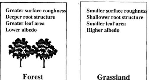
Some of the important characteristics of vegetation affecting energy fluxes are its

surface roughness, root structure/rooting

depth, leaf area, and albedo. Figure 2-1

summarizes the different characteristics of forest and grassland and the effects of

these differences on local climate are discussed below using the example of large scale

deforestation.

(35)

Greater surface roughness Deeper root structure Greater leaf area Lower albedo

Forest

Smaller surface roughnes~ Shallower root structure Smaller leaf area

Higher albedo

Grassland

Figure 2-1: Characteristics of vegetation which affect the surface energy balance.

amount of solar radiation which is absorbed at the surface. Forests, which typically

have lower albedos than grasslands, absorb more solar radiation. Forest albedos are

in the range 12% - 14% while grassland albedos are in the range 16% - 19% (Culf et al.

1995, Bastable et al. 1993). Following deforestation, then, the land surface absorbs

significantly less solar radiation.

The cooling effect of the reduction in net solar radiation is counteracted by a

decrease in evaporative cooling following deforestation. Vegetation strongly affects

the partitioning of energy between latent and sensible heat fluxes. Because of their

greater leaf area index, more interception loss takes place from forests than from

grasslands. In addition to greater leaf area, trees also have deeper root structures

and are able to access deeper soil moisture or groundwater. Thus, transpiration

from forest can also exceed that from grassland. Also, because of the greater overall

height and variability in height of vegetation in a forest versus grassland, the surface

roughness is greater over forests than over grasslands. For all these reasons, total

evapotranspiration is usually greater from a forest than from a grassland, and over

forest the heat exchange between the land surface and the atmosphere is more strongly

dominated by latent heat fluxes than by sensible heat fluxes. Following deforestation,

(36)

of the deforested region as compared to the original forest.

The increased temperatures following deforestation results in increased outgoing

longwave radiation. In addition, decreased evapotranspiration implies a smaller

atmospheric water vapor content which will tend to diminish the greenhouse effect and

result in a smaller downwards longwave radiative flux. These two effects combine to

produce a smaller net longwave radiative flux following deforestation. This reduction

is combined with the reduction in net solar radiation and results in a reduction in the

net allwave radiation. As noted by Eltahir (1996), since the net all wave radiation is

the sum of the inputs of energy into the surface, the net allwave radiation must be

balanced by fluxes of sensible and latent heat which expel energy into the atmosphere.

As already noted, deforestation induces a reduction in latent heat fluxes. Higher

temperatures following deforestation imply an increase in the sensible heat flux and

the depth of the boundary layer. Thus, a smaller amount of energy is spread over

a larger depth of the boundary layer following deforestation and we can expect that

over grassland the moist static energy, or boundary layer entropy is smaller than over

forest. This reduces the likelihood of local convective precipitation.

The change in evapotranspiration also affects the movement of moisture from the

land surface to the atmosphere, which has important implications for atmospheric

dynamics. Decreased atmospheric moisture and diminished convective activity

suggest that cloudiness will also decrease following deforestation. Decreased

cloudiness would increase the downwards shortwave radiative flux at the surface

but decrease the downwards longwave radiative flux at the surface. Numerical

modeling studies of large scale Amazonian deforestation (e.g., Dickinson and Kennedy

(1991) and Lean and Rowntree (1993)) support this view. The actual consequence

of deforestation on cloudiness, however, is likely to depend upon the scale of the

deforested region. Observational studies have indicated that reduced vegetative cover

at smaller scales may actually increase shallow cumulus cloud cover. For example,

Cut rim et al. (1995) presented data showing an increase in dry-season afternoon

fair-weather cumulus clouds over deforested regions in Amazonia. Rabin and Martin

(37)

lightly vegetated versus heavily vegetated landscapes during a drought year in the

midwestern United States.

It

should be noted that the increase in cloud cover in both

these studies were observed during dry periods. Again, the scale of the vegetation

change is an important consideration, and at the large scales considered in this study,

deforestation is expected to result in diminished cloud cover.

In summary then, deforestation results in increased surface albedo and reduced

absorbed solar radiation (cooling trend), decreased net longwave radiation (cooling

trend), and decreased evapotranspiration (heating trend). The effects of deforestation

on cloudiness depend upon the scale of deforestation. The balance of these competing

effects have been studied in numerous modeling studies of large scale Amazonian

deforestation. These studies generally agree that the net effect of deforestation is a

warming of the near surface climate and a decrease in precipitation (e.g., Lean and

\Varrilow, 1989; Shukla and Sellers, 1990; Dickinson and Kennedy, 1992;

Henderson-Sellers et aI, 1993; Eltahir and Bras, 1994; and Lean and Rowntree, 1997). The

reduction in precipitation can be attributed to a reduction in atmospheric moisture

convergence and a reduction in evaporation leading to reduced precipitation recycling.

Different studies have shown varying contributions

of these two mechanisms to

reduced precipitation. This is discussed further in Section 2.2.3.

At long time scales, vegetation has other indirect effects on climate. For example,

because vegetation serves as a large carbon storage reservoir, changes in vegetation

affect the global carbon balance. If less carbon is stored in vegetation and storage in

other reservoirs such as the ocean do not change, decreased vegetation implies that

carbon dioxide concentrations in the atmosphere will increase. As carbon dioxide is

an important greenhouse gas, changes in atmospheric carbon dioxide concentrations

can have important implications for global climate.

Vegetation and climate also both affect nutrient cycling in the soils. Vegetation

is dependent on the availability of nutrients in the soil. Nutrient availability is in

turn influenced by rates of decay and rates of microbial activity which may change

with climatic factors such as temperature and humidity. Hence, interactions between

vegetation, climate and nutrient cycling may be important.

(38)

Vegetation and climate both also affect soil erosion. Dense vegetation stabilizes

the soil matrix, helping to prevent excessive erosion. Characteristics of climate such

as the intensity and duration of rainfall events also affect erosion. For example, the

high intensity rain events in tropical areas could result in severe erosion if protective

vegetation cover is removed. Soil erosion can inhibit the reestablishment of vegetation,

and so the interaction between vegetation, climate, and soil erosion may also play an

important role in the biosphere-atmosphere system.

While these indirect effects may be quite important in determining the interaction

between vegetation and climate, they are beyond the scope of this study.

2.2.2 Observational studies

Observational studies have been conducted at paired forest and grassland sites

in the Amazon forest as part of the Amazon Region Micrometeorological

Experiment (ARME) and the Anglo-Brazilian Amazonian Climate Observation Study

(ABRACOS). A brief overview of some of the results of these studies in the context

of forest climate versus grassland climate is given here. These observations showed

that net allwave radiation (including both net longwave radiation and net shortwave

radiation) was smaller at the cleared sites, in accordance with the theory described

above. On average, the net allwave radiation was about 11% less at pasture sites

than at forest sites. However, there was no appreciable difference in mean annual

temperature and humidity between the forest and pasture sites (Culf et al. 1996).

Wright et al. (1992) observed a substantial decrease in evaporation (approximately

45% reduction) during the transition from the wet season to the dry season at a

ranchland site in central Amazonia. Based on these observations, they postulated

that the dry season evaporation at cleared sites is likely to differ significantly

from dry season evaporation over undisturbed forest. Indeed, Shuttleworth (1988) 's

observations of evaporation at a nearby forest site exhibited much less seasonality.

While the observed climatological differences over forest and grassland do not

match all of the expectations based on theory and modeling studies, this may be due

(39)

Table 2.1: Results from Modeling Studies of Amazonian Deforestation

Study

Lean and Warrilow (1989) Shukla et al. (1990)

Dickinson and Kennedy (1992)

Henderson-Sellers et al. (1993)

EI tahir and Bras (1994)

Lean and Rowntree (1997)

~T

[K]

+2.0 +2.5

+0.6

+0.7

+2.3

~p

[mm/day]

-1.3

-1.8

-1.4

-1.6

-0.4 -0.3

~E

[mm/day]

-0.6

-1.4 -0.1

-0.6

-0.8 ~Rn

[W/m2]

n/a -26 n/a n/a -13 n/a

and ABRACOS included both an extensive forest location and an extensive grassland

location. At the two other paired locations, one vegetation type was dominant in the

area. In such a scenario, development of separate boundary layers over forest and

grassland may not have taken place and there may have been significant horizontal

mixing of air over the contrasting vegetation types.

2.2.3 Previous modeling studies

As noted in Section 2.2.1, deforestation in the Amazon River basin has been the

subject of numerous modeling studies. Using regional climate models or global

atmospheric general circulation models (AGCM's), researchers have consistently

demonstrated that deforestation of the Amazon is likely to have significant impacts

on the regional climate. Most studies agree that large scale deforestation results

in less precipitation, less evaporation, and higher surface temperatures (e.g., Lean

and Warrilow, 1989; Shukla, Nobre and Sellers, 1990; Dickinson and Kennedy, 1992;

Henderson-Sellers et aI, 1993; Eltahir and Bras, 1994; and Lean and Rowntree, 1997),

as predicted by the theory discussed in the previous section. Table 2.1 summarizes

the key results of some of these studies.

However, there is some question as to whether deforestation will increase or

decrease moisture convergence, with differing results from different studies, as pointed

(40)

deduced from the change in the quantity (precipitation - evaporation).

Four of

the six studies listed in Table 2.1 show a larger decrease in precipitation than in

evaporation, implying a decrease in moisture convergence.

In contrast, the other

two show greater sensitivity of evaporation than precipitation to deforestation. This

implies that increased moisture convergence partly compensates for the reduction in

evaporation.

It

is unclear why these different studies predicted opposing responses in moisture

convergence.

The conflicting results may be due to differences in the details of

the representation of land surface characteristics and topography as discussed by

Lean and Rowntree (1997). Eltahir and Bras (1993b) point out that the change in

moisture convergence reflects changes in the large scale circulation of the region. The

circulation responds to two different processes - changes in precipitation and changes

in surface temperature.

The complexity of resolving these conflicting responses may

contribute to the differing signs in the predicted change in moisture convergence. As

the long term mean annual moisture convergence corresponds to the long term mean

annual runoff, the change in moisture convergence is an important quantity which

bears further study.

A number of studies have also investigated the effects of vegetation on climate in

the West Africa region. Xue et al. (1990) used a 2-D zonally averaged model to test

the response of climate in West Africa to removal and expansion of the Sahara Desert

during the monsoon season. An expansion of the desert to ION resulted in changes to

the July climate which included an average decrease in precipitation of 13% for their

entire model domain.

The largest changes were seen in the desertification region.

In this region, precipitation decreased by 1.5 mm/day, evaporation decreased by 1.7

mm/ day, and cloud cover decreased by 7%. In addition, the surface temperature

increased by about

lK.

When the desert was removed, i.e., vegetation was enhanced

in the Sahara region, precipitation increased by an average of 25% over the whole

model domain.

Over the Sahara region, the change was more dramatic, with an

increase in precipitation upwards of 300%. In this experiment, a dipole pattern in the

precipitaton change was seen, and south of the Sahara there was actually a decrease

(41)

in rainfall. Surface temperature decreased with the enhanced vegetation.

Xue and Shukla (1993) used a general circulation model to study the effects of

desertification on the summertime climate of West Africa. Again, rainfall was reduced

in the desertification area during the summer monsoon. In addition, a dipole pattern

was also seen, in which the reduction in rainfall in the north was accompanied by an

increase in rainfall to the south.

Zheng and

EI

tahir (1998) used a two-dimensional zonally symmetric model to

study the role of vegetation in the the dynamics of the West African monsoon. Their

model used a very simple scheme for representation of the land surface, using the

Budyko dryness index as an indicator of vegetation type. In a perpetual summer

experiment simulating deforestation from 5N - 15N, they found that August rainfall

in that region' was severely impacted by deforestation. The rainfall maximum at

12N was decreased by about one half and the moisture convergence was only about

one-third of the value in the control case, indicating a strong effect of vegetation on

the monsoon circulation. The location of the imposed vegetation change was seen to

strongly affect the magnitude of the climatic change. A desertification experiment

showed a smaller response of the summer monsoon to vegetation change in the region

north of 15N.

Other modeling studies have tested the sensitivity of climate to land surface

changes in extratropical regions. Bonan (1997) used the NCAR Community Climate

Model version 2 (CCM2) coupled to NCAR's Land Surface Model (LSM) to study the

climatic impact of the replacement of natural vegetation in the United States with

agriculture. Agriculture has generally replaced broadleaf deciduous trees, needleleaf

evergreen trees and grasses with crop vegetation, although there are exceptions such

as in the case of managed forest. Changes from forest to crop generally result

in reduced roughness length and reduced leaf and stem area index. While these

effects would tend to reduce evapotranspiration, agricultural crops typically have

lower stomatal resistances than other plant types. The net result is often to increase

evapotranspiration. Shifts to agriculture have had varying effects on surface albedo,

(42)

in the eastern United States may have resulted in a cooler springtime climate, due largely to increased latent heat flux and higher surface albedo. These two effects may

also have been responsible for a cooler summer over much of the United States in

his agricultural U.S. versus natural U.S. simulations. His model also showed changes

in precipitation and near-surface atmospheric moisture as a consequence of land use

changes.

2.3 Two-way feedbacks

2.3.1 Theory

Because vegetation both influences and is influenced by climate, there is the potential

for feedback loops in the vegetation-climate system. A shift in climate may encourage

the growth of a particular type of vegetation. If this vegetation type further enhances

the climate shift, the system may enter into a positive feedback loop. Conversely, the

change in vegetation may trigger a negative feedback, tending to bring the climate

(and eventually vegetation) back to its original state.

Charney (1975) 's classic paper on desertification provides an example of a possible

feedback between vegetation and climate. Relative to its surroundings, a desert

absorbs less solar radiation because of its high albedo. In addition, high surface

temperatures result in a large loss of longwave radiative energy. Consequently, a

desert is a radiative sink of energy relative to its surroundings. In order to maintain

thermal equilibrium, air must descend, resulting in adiabatic warming, over these

desert regions. This subsidence further suppresses precipitation, further discouraging

the growth of vegetation, in a positive feedback loop. Charney demonstrated this

phenomenon in a simple zonal model of the atmosphere.

Over rainforest, the opposite effect encourages precipitation and vegetation

growth. Relative to its surroundings, the rainforest is a source of energy, owing to its

low albedo and low surface temperature. This creates conditions favoring convection

Biosphere-atmosphere interaction in a one-dimensional climate model of the tropics

Biosphere-Atmosphere

Interaction in a

One-Dimensional

Climate Model of the Tropics

by

Julie E. Kiang

Submitted to the Department

of Civil and Environmental

Engineering

in partial fulfillment of the requirements for the degree of

Master of Science in Civil and Environmental

Engineering

at the

MASSACHUSETTS

INSTITUTE

OF TECHNOLOGY

January

1999

[ Fe6YV1

U) /9!Jj]

@

Massachusetts

Institute

of TecHnology 1999. All rights reserved.

Author...

.

.

DwaI/tment

of Civil and EnvironmeIitat'Engineering

January

15, 1999

Certified by ....

Elfatih A.B. Eltahir

Associate Professor

Thesis Supervisor

Accepted by

'~ ..~

"

.

Andrew J. Whittle

Chairman, Department

Committee on Graduate

Students

Biosphere-Atmosphere Interaction in a One-Dimensional

Climate Model of the Tropics

by

Julie E. Kiang

Abstract

Acknowledgments

Contents

Introduction

2 Biosphere - Atmosphere Interactions

29

3

Climatology and Ecology of West Africa

51

Model Description

Coastal Domain: Experimental Simulations

89

6 Inland Domain: Experimental Simulations

165

7

Conclusion

A Biomass Initialization

185

190

190

193

205

210

211

List of Figures

/m

1m2],

[W

1m

[W

1m

[JIkg/K],