Automatic detection of code-switching in Arabic dialects

Automatic Detection of Code-switching in Arabic

Dialects

by

Gabrielle Cristina Rivera

Submitted to the Department of Electrical Engineering and Computer

Science

in partial fulfillment of the requirements for the degree of

Master of Engineering in Electrical Engineering and Computer Science

at the

MASSACHUSETTS INSTITUTE OF TECHNOLOGY

June 2019

c

Massachusetts Institute of Technology 2019. All rights reserved.

Author . . . .

Department of Electrical Engineering and Computer Science

June 7, 2019

Certified by . . . .

James Glass

Senior Research Scientist

Thesis Supervisor

Certified by . . . .

Suwon Shon

Research Scientist

Thesis Supervisor

Accepted by . . . .

Katrina LaCurts

Chair, Master of Engineering Thesis Committee

Automatic Detection of Code-switching in Arabic Dialects

by

Gabrielle Cristina Rivera

Submitted to the Department of Electrical Engineering and Computer Science on June 7, 2019, in partial fulfillment of the

requirements for the degree of

Master of Engineering in Electrical Engineering and Computer Science

Abstract

Multilingual and multidialectal speakers commonly switch between languages and di-alects while speaking, leading to the linguistic phenomenon known as code-switching. Most acoustic systems, such as automatic speech recognition systems, are unable to robustly handle input with unexpected language or dialect switching. Generally, this results from both a lack of available corpora and an increase in the difficulty of the task when applied to code-switching data.

This thesis focuses on constructing an acoustic-based model to gather code-switching information from utterances containing Modern Standard Arabic and dialectal Ara-bic. We utilize the multidialectal GALE Arabic dataset to classify the code-switching style of an utterance and later to detect the location of code-switching within an ut-terance. We discuss the failed classification schemes and detection methods, providing analysis for why these approaches were unsuccessful. We also present an alignment-free classification scheme which is able to detect locations within an utterance where dialectal Arabic is likely being spoken. This method presents a marked improvement over the proposed baseline in average detection miss rate. By utilizing this informa-tion, Arabic acoustic systems will be more robust to dialectal shifts within a given input.

Thesis Supervisor: James Glass Title: Senior Research Scientist Thesis Supervisor: Suwon Shon Title: Research Scientist

Acknowledgments

First, I would like to thank my thesis advisors, Jim Glass and Suwon Shon. They provided me with invaluable guidance, advice, and ideas over the past year. I con-sider myself very lucky to have been able to work with and learn from them. I would also like to thank the entire Spoken Language Systems group for cultivating an environment of collaboration and making my Meng experience both enjoyable and educational. Furthermore, the work detailed in this thesis could not have been com-pleted without the help of our colleagues at the Qatar Computing Research Institute. A special thank you to Ahmed Ali for quick answers to all my questions, despite the seven-hour time difference.

I owe a big thank you to my parents for always being only one phone call away. They have always believed in me and their support means the world to me. I also want to thank my little sister and wish her luck as she begins the journey I am now concluding. Lexi, you are strong and wise and I am very proud of you. I have taught you everything I know, and you have become a far greater Jedi than I could ever hope to be.

Lastly, but most importantly, I would like to thank my dog, Gracee, for her infectious happiness and unconditional love.

Contents

2.1.1 Non-Computational and Linguistic Work . . . 19

2.1.2 Natural Language Processing Work . . . 20

2.1.3 Acoustic Work . . . 22

2.2 Speech-based Work . . . 23

2.2.1 Modeling Unsegmented Data . . . 23

2.2.2 Spoken Term Detection . . . 24

2.2.3 Language and Dialect Identification . . . 24

3 Code-switching Speech Data 27 3.1 GALE Dataset . . . 28

3.1.1 The Full Dataset . . . 29

3.1.2 The Reduced Dataset . . . 29

4 Preliminary Experiments 33 4.1 Code-Mixing Index . . . 33

4.1.1 Data Processing . . . 33

4.1.2 Classifiers . . . 35

4.1.3 Evaluation and Results . . . 37

4.1.4 Conclusions . . . 40

4.2 Binary Classification . . . 42

4.2.1 Data Processing . . . 42

4.2.2 Neural Network Classifier . . . 43

4.2.3 Evaluation and Results . . . 44

4.2.4 Conclusions . . . 45

5 Alignment-Free Code-switching Detection System 47 5.1 Data Processing . . . 47

5.1.1 Feature Extraction . . . 48

5.1.2 Classification . . . 48

5.2 Bi-LSTM + Attention Classifier . . . 48

5.2.1 Bi-LSTM . . . 48

5.2.2 Attention Module . . . 49

5.3 Alignment-Free Training . . . 50

5.4 Further Processing and Peak Detection . . . 51

5.5 Evaluation . . . 53

5.5.1 Metrics . . . 53

5.5.2 Results . . . 54

5.5.3 Attention Module Analysis . . . 55

5.6 Conclusions . . . 57

6 Conclusions 59 6.1 Summary of Contributions and Findings . . . 59

List of Figures

4-1 General architecture of the model proposed in (Yu et al., 2018), where T represents the time dimension, X represents the size of the input features, and H represents the size of the hidden states. Final Log-Softmax activation is not shown. . . 37 4-2 Architectures of the three attention module variations tested in this

preliminary experiment. The leftmost branch displays the model with no added attention, the center branch displays the single-level attention module, and the rightmost branch displays the multi-level attention module. Final LogSoftmax activation is not shown. Input labels to the attention modules correspond to labels in Figure 4-1. . . 38 4-3 Frame-level binary label extraction process. Word-level labels were

generated using the transcripts as well as the timestamp and duration information provided by the forced word alignment file. Frames were then mapped to word-level labels based on the start of the frame. . . 43 4-4 NN classifier architecture. The convolutional layer utilizes a kernel size

of 25. Final LogSoftmax activation is not shown. . . 44 4-5 Two examples of DA class probability outputs from different

utter-ances as well as their associated ground truth labelings. A value of 1.0 represents the DA class and a value of 0.0 represents the MSA class. . 46

5-1 Bi-LSTM + Attention architecture. In implementation, the hidden dimension of the bi-LSTM layer, H, is of size 100. Final LogSoftmax activation is not shown. . . 49

5-2 Example DA probability estimates for a single utterance. . . 52 5-3 Filtered DA probability estimates for the same utterance shown in

Figure 5-2. Detected peaks are marked in red. . . 52 5-4 Two examples of filtered DA probability estimates and detected peaks

as well as ground truth labelings. . . 55 5-5 Two examples of attention vector values and the associated ground

truth labelings for the utterance. Downward spikes in the attention vector tend to occur at the beginning or end of DA segments. . . 57

List of Tables

2.1 An example sentence containing code-switching that adheres to the equivalence constraint proposed in Poplack’s Model. The switch occurs in a location within the utterance where the grammatical structures of both English and Spanish align. The example is translated to both English and Spanish below the original utterance for clarity. . . 21

2.2 An example sentence containing code-switching that adheres to the Matrix language-frame model. In this instance English represents ma-trix language and Spanish represents the embedded language. Two Spanish phrases, “por favor” and “las floras” are inserted into the English-dominated utterance. The example is translated to both En-glish and Spanish below the original utterance for clarity. . . 21

3.1 Size and code-switching statistics for the full dataset. The discrepancy between Total Size and the breakdown of Total Size by dialect is due to the use of the forced word alignments in the calculation of Total MSA Size and Total DA Size. The forced word alignments cut out time containing silence in an utterance. The Total Size takes into account time due to silence. . . 29

3.2 Total DA size breakdown by dialect for the full dataset. The Levantine dialect data consists of broadcasts from Jordan, Lebanon, and Syria; the Gulf dialect data consists of broadcasts from Iraq, Kuwait, Oman, Qatar, Saudi Arabia, and the UAE; the Egyptian dialect consists of only broadcasts from Egypt; the other category contains broadcasts collected from the non-Arabic speaking countries of Iran and the US. 30

3.3 Size and code-switching statistics for the reduced dataset. The discrep-ancy between Total Size and the breakdown of Total Size by dialect is due to the use of the forced word alignments in the calculation of Total MSA Size and Total DA Size. The forced word alignments cut out time containing silence in an utterance. The Total Size takes into account time due to silence. . . 31

3.4 Total DA size breakdown by dialect for the reduced dataset. The Lev-antine dialect data consists of broadcasts from Jordan, Lebanon, and Syria; the Gulf dialect data consists of broadcasts from Iraq, Kuwait, Oman, Qatar, Saudi Arabia, and the UAE; the Egyptian dialect con-sists of only broadcasts from Egypt; the other category contains broad-casts collected from the non-Arabic speaking countries of Iran and the US. . . 31

4.1 CMI values and size by CMI classes for the full dataset. . . 35

4.2 Baseline results for the Code-Mixing Index experiment. Results were obtained by classifying each utterance as CMI1, the majority class. Overall accuracy and precision, recall, F1 scores by CMI class are dis-played. Calculated using the full dataset test set. . . 38

4.3 Overall accuracy and precision, recall, F1 scores by CMI class. Cal-culated at the utterance-level using the GMM-UBM classifier and the full dataset test set. . . 39

4.4 Results for the NN model with no added attention, trained on utterance-level dialect embeddings and phoneme frequency embeddings. Overall accuracy and precision, recall, F1 scores by CMI class are displayed. Calculated at the utterance-level using the full dataset test set. . . 39 4.5 Results for the NN model with no added attention, trained on 250

ms interval dialect embeddings and phoneme frequency embeddings. Overall accuracy and precision, recall, F1 scores by CMI class are dis-played. Calculated at the utterance-level using the full dataset test set. . . 40 4.6 Results for the NN model with the multi-level attention module, trained

on 250 ms interval dialect embeddings. Overall accuracy and preci-sion, recall, F1 scores by CMI class are displayed. Calculated at the utterance-level using the full dataset test set. . . 40 4.7 Baseline results for the binary classification experiment. Results were

obtained by labeling each frame as MSA, the majority class. Overall accuracy and precision, recall, F1 scores by dialect class are displayed. Calculated at the frame-level using the reduced dataset test set. . . . 44 4.8 Results for the CNN model using the classification threshold described

in (4.2). Overall accuracy and precision, recall, F1 scores by dialect class are displayed. Calculated at the frame-level using the reduced dataset test set. . . 45

5.1 Baseline results for the metrics used to evaluate the alignment-free code-switching detection system. Results were obtained by labeling each word as MSA or DA based on the class distribution of the reduced dataset training set. FAR, MR, and PHR were calculated for each utterance and then averaged. . . 54 5.2 Results of the alignment-free code-switching detection system

calcu-lated for N = 0, 10, 25. FAR, MR, and PHR were calcucalcu-lated for each utterance in the reduced dataset test set and then averaged. . . 54

5.3 Results of the binary classifier, described in Section 4.2, calculated for N = 0, 10, 25. FAR, MR, and PHR were calculated for each utterance in the reduced dataset test set and then averaged. . . 55 5.4 Results of the alignment-free code-switching detection system with the

attention module removed. Calculated for N = 0, 10, 25. FAR, MR, and PHR were calculated for each utterance in the reduced dataset test set and then averaged. . . 56

Chapter 1

Introduction

1.1

Code-switching

Code-switching is a linguistic phenomenon in which a speaker shifts between two or more languages or dialects while speaking. This type of speech is commonly found in multilingual societies and areas where dialectal variations of a language are frequently used, such as India and many Arabic-speaking nations. Switching between codes in a single conversation can occur for a variety of reasons. Speakers may switch to a new code due to lexical need or in order to compensate for shortcomings of the previously used language or dialect. The tone or topic of a conversation may also shift, provoking a change to a code which better fits the new direction of the dialogue. In all cases, code-switching is dependent on many situational variables, making it difficult to speculate when and where it may arise. In recent years, code-switching has become increasingly more common due to globalization and the widespread use of social media. These and many other factors have brought about the integration of lingua francas into native languages, as well as normalized the mixing of colloquial dialects with standard language.

Language or dialect shifts in day-to-day speech can be grouped into three pri-mary categories: inter-sentential, code-switching between utterances; intra-sentential, code-switching within a single utterance; or intra-word, code-switching within a sin-gle word. Most studies on code-switching focus on intra-sentential switching, due to

the interesting linguistic elements which commonly emerge during the speech. Ex-amples of this include alternations, the alternation and combination of two separate grammars, and insertions, insertion of features from one code into another.

1.2

Code-switching in Arabic

Code-switching is especially common in Arabic-speaking countries. The reasons for this trace back over a thousand years to the birth of Islam in the 7th century CE. The spread of Islam led to the unification of many previously divided nations within the Middle East. Tribes from the Arabian Peninsula headed conquests across the area, propagating religious teachings to local peoples and causing sweeping political changes. Linguistically, these conquests introduced an early form of Arabic, known as Classical Arabic, to many new peoples. The caliphs of the Arab dynasty estab-lished schools to teach Classical Arabic and Islam by means of the Quran, the central religious text of Islam written in Classical Arabic. By the 8th _{century CE, the}

stan-dardization of Classical Arabic had reached completion and knowledge of the language became essential for academics and individuals of the Arab world who wished to im-prove or maintain high societal positions. However, in everyday life, it was common for individuals to continue speaking languages native to their nation or combine their first languages with Classical Arabic, creating a variety of colloquial Arabic dialects. Roughly a thousand years later, colonization of the Arab world by European countries further influenced the linguistic history of the area. During the era of colonization, French and English were often used in schools, rather than Arabic. The knowledge of such European languages was seen as a badge of sophistication and necessary for educated individuals. Many countries previously under colonial occupation still formally learn the languages of their earlier colonial rulers. These centuries of European influence have brought about the borrowing and integration of western languages into local Arabic dialects.

Unlike many modern languages, which while containing dialects tend to be more universally defined, Arabic is more akin to a lingua franca of the Arab World.

Tech-nically, Arabic is classified as a macrolanguage, encompassing 30 modern varieties as well as Modern Standard Arabic (MSA). Many of these varieties or dialects are mu-tually unintelligible and considered completely separate languages by some linguists. MSA is widely utilized in schools, formal situations, written media, and as a lingua franca to help speakers of different dialects communicate. Consequently, Arabic has emerged as a prime example of the linguistic phenomenon diglossia: the normal use of two separate varieties of a language, typically used in different social situations. Individuals commonly need to switch between their native dialect and MSA in order to communicate with speakers of different dialects.

The rise of Islam and subsequent era of western colonization has produced a unique linguistic situation in the area. Code-switching is a frequent and necessary phenomenon; making Arabic an excellent language choice for work in this linguistic area.

1.3

The Problem

In the past decade, the use of acoustic systems, such as Text to Speech (TTS) and Automatic Speech Recognition (ASR) systems, has greatly increased. Similarly, code-switching is quickly becoming more widely used and accepted in modes of communica-tion other than informal speech. Many of the acoustic systems previously mencommunica-tioned are trained using data from a single language or dialect. Monolingual and monodi-alectal speech data is the most widely available and therefore the most commonly used. However, this leads to the creation and use of acoustic systems which cannot robustly handle input with unexpected language or dialect switching.

The work in this thesis focuses on constructing an acoustic-based model to gather code-switching information. Specifically, the model will aim to gather information pertaining to the location of code-switching points within utterances containing MSA and various Arabic dialects. The model will be limited to using only features which can be easily extracted from acoustic data. Ultimately, the information obtained from this model will be available for use by other acoustic systems in order to improve

performance on code-switching input data.

1.4

Thesis Outline

The contributions of this work are centered around exploring what type of informa-tion about code-switching can be automatically gathered by a model, when provided with only an acoustic representation of an utterance. Although focused on switch-ing between MSA and dialectal Arabic (DA), the findswitch-ings of this research should be applicable to intra-sentential code-switching in different languages and dialects.

The remainder of this thesis is organized as follows: Chapter 2 discusses the background and related work utilized while conducting this research. Chapter 3 introduces the GALE dataset. Chapter 4 discusses preliminary experiments and their important findings. Chapter 5 describes the implementation of the current system and provides an evaluation of said system. Chapter 6 offers concluding remarks and possible future avenues for this work.

Chapter 2

Related Work

There has been very little research conducted on acoustic code-switching data and the potential to integrate this data into other types of acoustic systems. Due to this, the previous work used for reference in this thesis consists mainly of code-switching work done in other fields as well as speech-based research which closely relates or can somehow be applied to this task.

2.1

Code-switching Work

2.1.1

Non-Computational and Linguistic Work

The first recorded observations of code-switching by linguists occurred in the early 20th century. Jules Ronjat, a French linguist, is credited with making the earliest recorded observation in 1913 (Ronjat, 1913). Ronjat conducted a case study on his own son during his early years of life. The goal of the study was to successfully teach the boy French and German simultaneously, as first languages. At the time learning two languages from infancy was thought to distort the absorption of one or both of the languages. Ronjat created a technique referred to as one person, one language. For this technique he only spoke French to his son and his wife only spoke German. Ronjat strictly adhered to this practice. According to the study, code-switching between the two languages naturally arose in his son’s speech. However,

Ronjat and his wife refused to acknowledge any utterance which included mixing of the two languages, due to the stigma around dual language absorption.

In the following decades linguists continued to neglect code-switching as an inter-esting, potential area of work. Seeing it instead as a substandard use of language and the result of imperfect second language learning. Most scholars at the time did not believe a discernible pattern or logic could be applied to the phenomenon.

In the 1970s the scientific perspective on code-switching began to change. (Blom, 1972) published a survey in which they studied a Norwegian village that spoke two different dialects. The inhabitants of this village switched between the two dialects based on the social context of the conversation. After publication of this research, academic interest in code-switching began to grow. Scholars began searching for sys-tematic patterns and trying to create accurate models to predict when code-switching might occur and how language grammars mix.

Two popular models emerged from this early linguistic work. Poplack’s Model (Poplack, 1978) and the Matrix language-frame model (Myers-Scotton, 1997). Poplack’s model proposed the equivalence constraint, a rule stating that code-switching occurs only at points where the structures of the two codes coincide. In other words, where the general grammar or sentence element ordering match, leading to a smooth transi-tion between the codes. Figure 2.1 provides an example of this form of code-switching. The Matrix language-frame model presents the idea of a matrix language (ML) and an embedded language (EL). In this model the ML represents the dominant language. The grammar of the sentence adheres to that of the ML and elements of the EL are inserted into the ML. Figure 2.2 provides an example of this form of code-switching.

2.1.2

Natural Language Processing Work

The first computational approach to code-switching is attributed to (Joshi, 1982). (Joshi, 1982) developed a grammar-based system focusing on parsing and generating code-switched data in English and Marathi. Many recent approaches to processing code-switching data continue to use linguistic features to improve model performance. New research in computational approaches to detecting and utilizing code-switching

Language Type Example

Code-switching I like to read porque quiero ser un escritor. English I like to read because I want to be a writer. Spanish Me gusta leer porque quiero ser un escritor.

Table 2.1: An example sentence containing code-switching that adheres to the equiva-lence constraint proposed in Poplack’s Model. The switch occurs in a location within the utterance where the grammatical structures of both English and Spanish align. The example is translated to both English and Spanish below the original utterance for clarity.

Language Type Example

Code-switching Por favor, remember to buy las floras for Lexi’s graduation. English Please, remember to buy flowers for Lexi’s graduation. Spanish Por Favor, recuerda comprar las floras para la graduaci´on de Lexi. Table 2.2: An example sentence containing code-switching that adheres to the Matrix language-frame model. In this instance English represents matrix language and Span-ish represents the embedded language. Two SpanSpan-ish phrases, “por favor” and “las floras” are inserted into the English-dominated utterance. The example is translated to both English and Spanish below the original utterance for clarity.

data began to surface in the late 2000s. (Sinha and Thakur, 2005) proposed a system for machine translation of the commonly occurring Hinglish, code-switching between Hindi and English, to pure Hindi and pure English. (Solorio and Liu, 2008) published one of the first approaches to statistical detection of code-switching points for use in a part-of-speech tagger.

Severe lack of code-switching data and heightened interest in the phenomenon ul-timately led to the First Workshop on Computational Approaches to Code Switching in 2014 (Solorio et al., 2014). Team approaches were wide ranging; from a rule-based system that utilized character n-grams (Shrestha, 2014) to early attempts at inte-grating machine learning techniques, such as extended Markov Models (King et al., 2014) and support vector machines (Bar and Dershowitz, 2014).

In the past few years artificial neural networks (NNs) have emerged as the standard model of choice for natural language processing work. Specifically, the bidirectional long short-term memory network (bi-LSTM) has become one of the most popular

and successful NN architectures. During the Third Workshop on Computational Ap-proaches to Linguistic Code-switching (Aguilar et al., 2018), (Trivedi et al., 2018) obtained character representations via a convolutional neural network (CNN) and simultaneously generated word representations using a bi-LSTM. These representa-tions were passed to a dense conditional random field (CRF), which provided the final output prediction. (Wang et al., 2018) created a system for name entity recognition in code-switching data. They utilized a joint CRF-LSTM model with attention at the embedding layer. This system performed particularly well on noisy dialectical Arabic data.

2.1.3

Acoustic Work

There is currently a severe lack of code-switching data, especially for speech-based corpora. Despite the lack of speech data, code-switching has presented itself as an im-portant aspect of language to consider when creating acoustic systems, such as TTS and ASR systems. (Liang et al., 2007) proposed a bilingual TTS system that utilized a single speaker and a shared phone set to increase the quality of mixed-language synthesis. (Modipa et al., 2013) discussed the challenges of frequent Sepedi-English code-switching, in South Africa, on the accuracy of ASR systems. Code-switching data is especially challenging for speech systems to handle as acoustic models, pro-nunciation models, and language models may need to be redesigned in order to ac-commodate words from different codes. One common way to avoid this obstacle is to detect the locations of code-switch points and apply the correct models based on the detected switch points. (Chan et al., 2004) produced a system that utilized bi-phone probabilities to detect language boundaries between Cantonese and English. Similarly, (Lyu and Lyu, 2008) made use of acoustic, prosodic, and phonetic cues to detect language boundaries in Mandarin-Taiwanese code-switching speech.

More recently, (Yılmaz et al., 2016) utilized the FAME! corpus (Yilmaz et al., 2016) to engineer an ASR system for Frisian-Dutch code-switched speech. They initially trained a deep neural network (DNN) on Frisian, Dutch, and English mono-lingual data. After, they retrained the hidden layers of the DNN on a small amount

of monolingual Frisian data and a large amount of monolingual Dutch data. The code-switching data was only used for testing purposes, not in training. (Amazouz et al., 2019) conducted studies on the FACST corpus (Bougrine et al., 2017), con-taining French and Algerian Arabic code-switching speech. The majority of the work was focused on linguistic analysis of the data, followed by an initial attempt to locate code-switch points using word posteriors from an ASR system trained on the corpus. (Rallabandi et al., 2018) published one of the few experiments that utilized both code-switching data and DNN features in order to classify the “style” of code-code-switching within an utterance.

2.2

Speech-based Work

Although there is a lack of prior work in acoustic code-switching, there are similarities between other common tasks in speech-based research and code-switching.

2.2.1

Modeling Unsegmented Data

Many tasks containing sequential, unsegmented data necessitate the prediction of a se-quence of segmented labels. Common examples of this type of task include handwrit-ing recognition, optical action labelhandwrit-ing, and ASR. In both ASR and code-switchhandwrit-ing detection, unsegmented, acoustic data is provided to a system that is expected to parse this data into a sequence of distinct words or code labelings, respectively. These are difficult problems because they combine both the task of recognition and the task of segmentation.

In 2006, (Graves et al., 2006) published the Connectionist Temporal Classification (CTC) Algorithm. A loss function for training recurrent neural networks (RNNs) to predict sequences of labels with unsegmented input data. Graves tested his new algorithm on the temporal classification problem of phonetic labeling. The model, trained using CTC loss, was able to outperform the baseline as well as a similar model trained using traditional techniques. Since its initial publication, CTC loss has been utilized successfully in many unsegmented data tasks.

2.2.2

Spoken Term Detection

Automated code-switching detection, when viewed through the lens of the Matrix language-frame model, can be regarded as a spoken term detection task. Words or segments of the utterance from the EL represent the terms to be detected. Recently, (Ao and Lee, 2018) utilized an LSTM followed by an attention mechanism to deter-mine if a specific spoken term query exists in an audio segment. The LSTM was used as an acoustic encoder, while the attention mechanism was used to place attention on areas of the audio segment similar to the query. This model was able to outperform the same network without attention as well as the conventional dynamic time warping based approach.

2.2.3

Language and Dialect Identification

Many similarities can be drawn between code-switching tasks and language/dialect recognition tasks. These recognition tasks are popular in the field and have made effective use of deep learning systems.

Two main approaches to building NN-based systems for language and dialect identification have emerged over the past few years. The first utilizes a DNN to extract features from speech data, followed by a separate language or dialect classifier. (Jiang et al., 2014) created acoustic features, for use in language identification, by extracting “bottleneck” hidden layers of two separate monolingual-trained DNNs. The system constructed with these features was able to outperform the baseline. The second commonly used approach to deep learning systems utilizes a DNN to directly classify language or dialect. (Richardson et al., 2015) similarly experimented with mixing classical features/classifiers (Mel-frequency cepstral coefficients and Gaussian mixture models respectively) and NN-based features/classifiers (bottleneck features and DNN respectively) to predict the language of an audio segment from six possible tags.

Specialized DNNs have also proven to be very successful in language and di-alect identification. (Snyder et al., 2018) constructed a DNN, with a short temporal

context, for use in mapping acoustic features to fixed-dimension embeddings. The embeddings, referred to as x-vectors, were tested on identification of 14 different languages. They achieved good results, outperforming the state-of-the-art i-vector systems when using the same backend classifier. (Shon et al., 2018) built an end-to-end dialect identification system for Arabic dialects. They utilized four CNN layers followed by two fully-connected (FC) layers to create a language embedding vector. This vector was shown to successfully encode similarities between utterances of the same dialect and differences between utterances of different dialects. The end-to-end system outperformed i-vectors paired with cosine distance and Gaussian backend-to-end classifiers.

Chapter 3

Code-switching Speech Data

There are very few code-switching datasets available for use in acoustic systems. Moreover, the datasets that are available tend to contain small amounts of usable code-switching examples. This is partially due to the challenges that arise in the collection of this type of data. The number of potential speakers for use in data extraction is much smaller than for standard speech datasets, as code-switching only occurs in certain geographic areas and with certain multilingual or multidialectal speakers. Additionally, true code-switching speech must occur naturally; speakers cannot simply be given a transcript or story to read. The switch must be brought about by a naturally occurring event, such as the need for word in a different code or a shift in topic. Furthermore, code-switching still does not commonly occur in formal situations, making it difficult to quickly scrape the Internet for common speech sources, such as broadcast data. Some well-known code-switching datasets include the Miami Bangor corpus (Deuchar et al., 2014), the Mandarin-English Code-switching in South-East Asia corpus (Lyu et al., 2010), and the Frisian Audio Mining Enterprise corpus (Yilmaz et al., 2016). The work described in this paper focuses on code-switching between MSA and DA and makes use of the largest dataset available for this task: the GALE dataset (Walker et al., 2013a) (Walker et al., 2013b) (Walker et al., 2014).

3.1

GALE Dataset

The GALE Arabic dataset was collected over the course of two years, 2006-2007, as part of the DARPA GALE (Global Autonomous Language Exploitation) Program. The dataset contains transcribed acoustic broadcast data, featuring code-switching between MSA and various Arabic dialects. The data consist of a variety of differ-ent types of broadcast recordings, including interviews, listener call-ins, roundtable discussions, and report-style speech. Arabic-speaking countries represented in the dataset include Qatar, Jordan, Lebanon, Egypt, Oman, Saudi Arabia, Syria, the United Arab Emirates (UAE), Iraq, and Kuwait. Data was also collected from Ara-bic broadcasts originating in Iran and the United States (US).

The provided data includes audio recordings, presented in flac compressed Wave-form Audio File Wave-format (.flac) 16000 Hz single-channel 16-bit PCM, and transcripts. Transcript entries are made at the utterance level and were audited by a native speaker. Entries include the audio file containing the utterance, the start and stop time of the utterance within the audio file, speaker demographic information, segment type (e.g. report, conversational, etc.), and the transcription itself. The transcrip-tions are provided in Arabic script with DA segments marked using the start tag <non-MSA> and the end tag </non-MSA>.

In total 416 hours of broadcast data are included in the dataset. Of these 416 hours approximately 358 hours are comprised of utterances containing only MSA and no DA. An initial data cleaning was conducted by colleagues of the Spoken Language Systems group at the Qatar Computing Research Institute (QCRI). QCRI started by removing the 358 hours of MSA-only utterances from the dataset. Next, they created Buckwalter transliteration transcripts, forced word alignments, and phoneme alignments for the remaining utterances. Utilizing these additional resources provided by QCRI, we further separated the GALE dataset into two subsets: the full dataset and the reduced dataset. The full dataset contains all utterances from the GALE dataset after the initial MSA-only extraction done by QCRI (i.e. all utterances that are DA-only or contain code-switching). The reduced dataset was further filtered

by removing the DA-only utterances, leaving only utterances which contain code-switching.

3.1.1

The Full Dataset

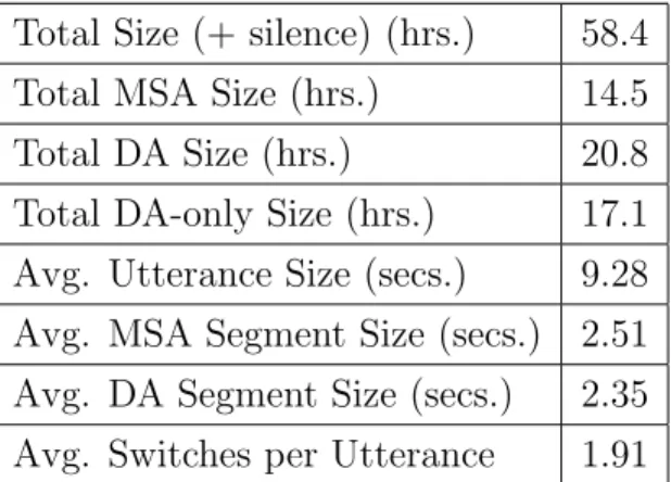
As previously mentioned, the full dataset contains all utterances in the GALE dataset other than MSA-only utterances. In total this is approximately 58.4 hours of audio data. Table 3.1 features more detailed statistics about this dataset. Interestingly, about one-third of this entire dataset consists of DA-only utterances, featuring no code-switching. The majority of DA data that appears in the dataset, about 82%, is found in these DA-only utterances. Levantine, Gulf, and Egyptian Arabic dialects appear in the data, with Levantine making up a large majority of the DA data. The size breakdown by dialect of the total spoken DA can be seen in Table 3.2. The most commonly occurring switching order of an utterance is DA-only, followed by: MSA-DA-MSA and MSA-DA-MSA-DA-MSA.

Total Size (+ silence) (hrs.) 58.4 Total MSA Size (hrs.) 14.5 Total DA Size (hrs.) 20.8 Total DA-only Size (hrs.) 17.1 Avg. Utterance Size (secs.) 9.28 Avg. MSA Segment Size (secs.) 2.51 Avg. DA Segment Size (secs.) 2.35 Avg. Switches per Utterance 1.91

Table 3.1: Size and code-switching statistics for the full dataset. The discrepancy between Total Size and the breakdown of Total Size by dialect is due to the use of the forced word alignments in the calculation of Total MSA Size and Total DA Size. The forced word alignments cut out time containing silence in an utterance. The Total Size takes into account time due to silence.

3.1.2

The Reduced Dataset

Due to the large percentage of non-code-switching data found in the full dataset, a new dataset was created by filtering out the DA-only utterance data. Thus, this subset of

Dialect Size (hrs.) Levantine 16.3 Gulf 3.16 Egyptian 0.76 Other 0.58

Table 3.2: Total DA size breakdown by dialect for the full dataset. The Levantine dialect data consists of broadcasts from Jordan, Lebanon, and Syria; the Gulf dialect data consists of broadcasts from Iraq, Kuwait, Oman, Qatar, Saudi Arabia, and the UAE; the Egyptian dialect consists of only broadcasts from Egypt; the other category contains broadcasts collected from the non-Arabic speaking countries of Iran and the US.

data represents all utterances containing code-switching from the original 416 hours of GALE data. After the removal of all monodialectal utterances, the dataset is left with approximately 37.6 hours of audio data. Table 3.3 features detailed statistics about the dataset. As expected, due to the removal of DA-only utterances, the total amount of spoken DA significantly decreased and the average number of switches per utterance increased. The average length of spoken DA segments also drastically decreased from over two seconds to about half a second; making DA segments, on average, much shorter than MSA segments. Once again, Levantine, Gulf, and Egyptian Arabic dialects appear in the data, with a Levantine majority. The size breakdown by dialect of the total spoken DA can be seen in Table 3.4. The most common utterance switching orders in the reduced dataset are: MSA-DA-MSA, MSA-DA-MSA-DA-MSA, and DA-MSA.

Total Size (+ silence) (hrs.) 37.6 Total MSA Size (hrs.) 14.5 Total DA Size (hrs.) 3.74 Avg. Utterance Size (secs.) 9.15 Avg. MSA Segment Size (secs.) 2.51 Avg. DA Segment Size (secs.) 0.56 Avg. Switches per Utterance 2.93

Table 3.3: Size and code-switching statistics for the reduced dataset. The discrepancy between Total Size and the breakdown of Total Size by dialect is due to the use of the forced word alignments in the calculation of Total MSA Size and Total DA Size. The forced word alignments cut out time containing silence in an utterance. The Total Size takes into account time due to silence.

Dialect Size (hrs.) Levantine 2.71 Gulf 0.79 Egyptian 0.12 Other 0.12

Table 3.4: Total DA size breakdown by dialect for the reduced dataset. The Levantine dialect data consists of broadcasts from Jordan, Lebanon, and Syria; the Gulf dialect data consists of broadcasts from Iraq, Kuwait, Oman, Qatar, Saudi Arabia, and the UAE; the Egyptian dialect consists of only broadcasts from Egypt; the other category contains broadcasts collected from the non-Arabic speaking countries of Iran and the US.

Chapter 4

Preliminary Experiments

4.1

Code-Mixing Index

The first approach taken in this work aimed to classify utterances from the dataset based on their code-mixing style. This classification approach was also used in the previously mentioned work (Rallabandi et al., 2018).

4.1.1

Data Processing

The code-mixing index experiment utilized the full dataset. The dataset was first divided into separate train, validation, and test sets using a 70/15/15 percentage split.

Feature Extraction

Four different types of features were extracted from the data: Mel-frequency cep-stral coefficients (MFCCs), dialect embeddings, one-hot phoneme embeddings, and phoneme frequency embeddings. The MFCCs and Mel-scaled spectrograms, used in the creation of the dialect embeddings, were obtained using the acoustic processing software Librosa1 _{(McFee et al., 2015).}

60-dimension MFCC features, including deltas and delta-deltas, were generated

1

using a 25 ms window and 10 ms stride. The dialect embedding features consisted of bottleneck features (BNFs) extracted from the end-to-end dialect identification system presented in (Shon et al., 2018). Two different sets of dialect embeddings were extracted from the data, varying in dimension. One at the utterance-level, with no time dimension, and one at intervals with 250 ms windows and 250 ms strides. For the utterance-level embeddings, a 40-dimension log Mel-scaled spectrogram was computed from the acoustic utterance data using a 32 ms window and 10 ms stride. These acoustic features were then used as input to the end-to-end model. A 600-dimension dialect embedding vector was then extracted from the second FC layer in the model. A very similar approach was used for the interval-based dialect embedding. A 40-dimension log Mel-scaled spectrogram was computed for each 250 ms interval of the utterance, using a 32 ms window and 10 ms stride. These acoustic features were passed to the model and a 600-dimension dialect embedding vector was extracted from the second FC layer of the model. The dialect embeddings for each 250 ms interval were then stacked along a time axis. After extraction both the utterance-level and interval-based dialect embeddings were normalized. Due to the nature of the end-to-end dialect identification model, it was thought these BNFs might encode useful information about the dialects present in an utterance.

The final two types of features extracted from the data were one-hot phoneme em-beddings and phoneme frequency emem-beddings. A phoneme recognizer (Schwarz, 2009) was run in order to label the data based on 60 possible phonemes. The 60-dimension one-hot phoneme embeddings were generated by simply indicating phonemes that appeared in a segment of interest. The 60-dimension frequency phoneme embeddings were generated by recording the frequency with which a phoneme appeared in a seg-ment of interest. Similar to the dialect embeddings, both types of phoneme features were extracted at the utterance-level and at 250 ms intervals.

Classification

Mirroring the recent work done by (Rallabandi et al., 2018), we utilized the Code-Mixing Index (CMI) measure, presented in (Gamb¨ack and Das, 2014), as a

classifica-tion scheme. CMI measures the amount of code-switching that occurs within a single utterance or corpus. The CMI value for an utterance, x, is defined as:

CM I(x) = 100 ∗ 0.5 ∗ (N (x) − M (x)) + 0.5 ∗ P (x)

N (x) (4.1)

where N(x) is the total number of words in the utterance, M(x) is the number of words in the most represented language or dialect, and P(x) is the number of code-switch points in the utterance.

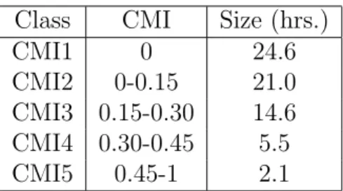
The CMI values for each utterance were calculated and then normalized to fall within the range [0, 1]. Utterances were then placed into five possible classes ranging from CMI1 to CMI5; where CMI1 represented a monodialectal utterance and CMI5 represented an utterance with frequent code-switching. Table 4.1 displays statistics for the data separated out by CMI class. As mentioned in Section 3.1.1, there is a heavy imbalance in the data. Approximately one-third of the entire dataset falls into the CMI1 class. Relative to CMI1, there are very few samples in the CMI4 and CMI5 classes.

Class CMI Size (hrs.) CMI1 0 24.6 CMI2 0-0.15 21.0 CMI3 0.15-0.30 14.6 CMI4 0.30-0.45 5.5 CMI5 0.45-1 2.1

Table 4.1: CMI values and size by CMI classes for the full dataset.

4.1.2

Classifiers

GMM-UBM Classifier

A simple GMM-UBM classifier was used to obtain a baseline result to further build from. The MFCC features described above were used as input to the model. All data from the training set was first used to fit a GMM-UBM with 512 components. Training data from each CMI class was then used for maximum a posteriori adaptation

of the GMM-UBM µ values. This resulted in five separate GMMs, one fit to each CMI class.

Neural Network Classifier

After obtaining an initial baseline result from the simple GMM-UBM classifier, ex-periments began with a more sophisticated NN model. This initial NN model was based on a previously successful acoustic model presented in (Yu et al., 2018). (Yu et al., 2018) designed a model for the weakly labelled classification problem presented by the Audio set dataset (Gemmeke et al., 2017). The objective of this task is to detect the presence or absence of 527 possible audio events within an audio clip. The general model is composed of three FC layers, which make up the embedding module, followed by an attention module (Figure 4-1). This model and all later NN models de-scribed in this thesis were created using the deep learning software PyTorch2 (Paszke et al., 2017).

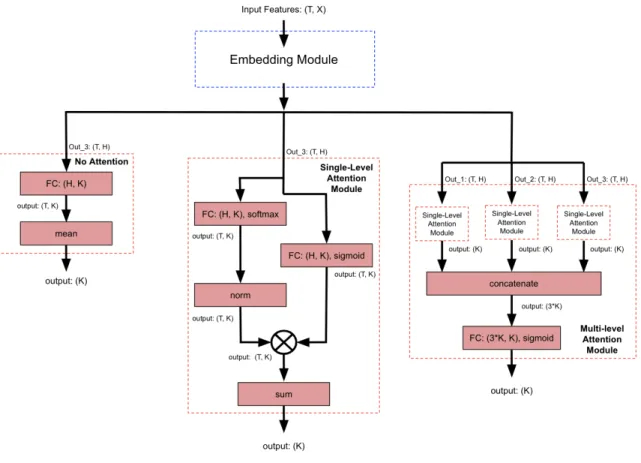
A variety of experiments were conducted using different feature inputs, variations on the NN model, and altered training procedures. The dialect embedding, one-hot phoneme, and frequency phoneme features, at both the utterance-level and 250 ms intervals, were utilized in this experiment. The performance of combinations of these features, such as utterance-level dialect embeddings concatenated with utterance-level one-hot phoneme embeddings, was also investigated. Additionally, three variations of the NN model were tested. These included the use of two different attention modules as well as the model with the attention module completely removed (Figure 4-2). The two possible attention modules included a single-level attention module and a multi-level attention module. The single-multi-level attention module is applied to the output of the embedding module. The multi-level attention module utilizes the hidden features from between the FC layers as well as the final output of the embedding module. Both attention modules were initially designed to aid the model in ignoring irrelevant segments from the audio clip, such as silence and background noise. Training was conducted using negative log likelihood (NLL) loss. Trials included varying the

learn-2

Figure 4-1: General architecture of the model proposed in (Yu et al., 2018), where T represents the time dimension, X represents the size of the input features, and H represents the size of the hidden states. Final LogSoftmax activation is not shown.

ing rate and weight decay as well as weighting the batch sampler and loss function based on the CMI class distributions in the training set.

4.1.3

Evaluation and Results

Final evaluation was conducted using the held-out test set for both classifiers. Exper-imental trial comparisons were conducted for the NN classifier using the validation set. Overall accuracy as well as class-level precision, recall, and F1 scores were calcu-lated at the utterance-level for each classifier. Naive baseline results were computed by classifying each utterance as the majority class in the dataset: CMI1. Table 4.2 contains the baseline results. The results obtained from both the GMM-UBM and NN classifier models were comparable to those found in the previous work. However, there was no significant improvement.

Figure 4-2: Architectures of the three attention module variations tested in this pre-liminary experiment. The leftmost branch displays the model with no added atten-tion, the center branch displays the single-level attention module, and the rightmost branch displays the multi-level attention module. Final LogSoftmax activation is not shown. Input labels to the attention modules correspond to labels in Figure 4-1.

Class Accuracy Precision Recall F1 CMI1 36.7% 0.367 1.0 0.537 CMI2 0.0 0.0 0.0 CMI3 0.0 0.0 0.0 CMI4 0.0 0.0 0.0 CMI5 0.0 0.0 0.0

Table 4.2: Baseline results for the Code-Mixing Index experiment. Results were obtained by classifying each utterance as CMI1, the majority class. Overall accuracy and precision, recall, F1 scores by CMI class are displayed. Calculated using the full dataset test set.

GMM-UBM Classifier

Each utterance was assigned a score for all five CMI classes based on its average frame log-likelihood for each of the adapted GMMs. The CMI class with the highest score

was then assigned as the predicted class of the utterance. The overall, utterance-level accuracy was 34.6%. Please refer to Table 4.3 for more detailed results.

Class Accuracy Precision Recall F1 CMI1 34.6% 0.567 0.428 0.488 CMI2 0.377 0.469 0.420 CMI3 0.290 0.167 0.212 CMI4 0.173 0.238 0.200 CMI5 0.147 0.314 0.200

Table 4.3: Overall accuracy and precision, recall, F1 scores by CMI class. Calculated at the utterance-level using the GMM-UBM classifier and the full dataset test set.

Neural Network Classifier

The best performing trial utilized the utterance-level dialect embedding concatenated with the utterance-level phoneme frequency embedding as input features. The model itself consisted of the embedding module with no added attention and was trained with a learning rate of 10−3, no weight decay, random batch sampling, and a weighted loss function. The overall, utterance-level accuracy was 38.9%. Please refer to Table 4.4 for more detailed results.

Class Accuracy Precision Recall F1 CMI1 38.9% 0.578 0.361 0.445 CMI2 0.474 0.522 0.497 CMI3 0.307 0.418 0.354 CMI4 0.188 0.260 0.218 CMI5 0.323 0.294 0.308

Table 4.4: Results for the NN model with no added attention, trained on utterance-level dialect embeddings and phoneme frequency embeddings. Overall accuracy and precision, recall, F1 scores by CMI class are displayed. Calculated at the utterance-level using the full dataset test set.

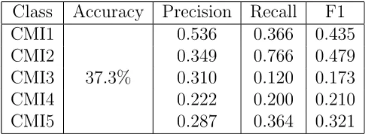
Trials which utilized the 250 ms interval-based features and two types of attention modules overall performed worse than the simpler trial described above. The overall, utterance-level accuracy of the interval-based features paired with the attention-less NN model was 37.3%; slightly worse than the best performing model. Please refer to Table 4.5 for more detailed results.

Class Accuracy Precision Recall F1 CMI1 37.3% 0.536 0.366 0.435 CMI2 0.349 0.766 0.479 CMI3 0.310 0.120 0.173 CMI4 0.222 0.200 0.210 CMI5 0.287 0.364 0.321

Table 4.5: Results for the NN model with no added attention, trained on 250 ms in-terval dialect embeddings and phoneme frequency embeddings. Overall accuracy and precision, recall, F1 scores by CMI class are displayed. Calculated at the utterance-level using the full dataset test set.

The attention modules function by applying attention to the embedded vectors in the time dimension. Thus, a trial utilizing both the utterance-level features and the attention modules could not be conducted. Trials were conducted utilizing the interval-based features and the NN model with single-level and multi-level attention. The best performing model with attention utilized the interval-based dialect embed-ding alone and the multi-level attention module. The overall, utterance-level accuracy was 43.3%. Please refer to Table 4.6 for more detailed results. Although the overall accuracy was higher than other models, the performance of this model on classes CMI4 and CMI5 was much worse.

Class Accuracy Precision Recall F1 CMI1 43.3% 0.468 0.733 0.571 CMI2 0.416 0.587 0.487 CMI3 0.304 0.152 0.203 CMI4 0.267 0.006 0.012 CMI5 0.425 0.070 0.120

Table 4.6: Results for the NN model with the multi-level attention module, trained on 250 ms interval dialect embeddings. Overall accuracy and precision, recall, F1 scores by CMI class are displayed. Calculated at the utterance-level using the full dataset test set.

4.1.4

Conclusions

The experiments conducted using the NN classifier provided interesting results that were further investigated prior to moving forward with this research. First, the slight decrease in performance between the utterance-level dialect embeddings and

the interval-based dialect embeddings was explored. In theory, the interval-based dialect embeddings should have provided the model with a finer-grained, more in-formative view of the utterance and thus, should have performed better. We closely inspected interval-based dialect embeddings that captured similar data. Embeddings of the same word or dialect should share more features than embeddings of separate dialects. However, very little correlation between theoretically similar embeddings was found. The model these embeddings were extracted from was trained to identify dialects given an entire utterance. Taking this into account, it seems likely that the embeddings are not reliable when the model is provided with a short speech segment, such as 250 ms.

The second result which was investigated was the decrease in performance when either the single-level or multi-level attention module was added. (Yu et al., 2018) designed the attention module to ignore segments of silence and background noise, while placing attention on segments with interesting noise features. However, when trained on the GALE data, the attention layer tended toward placing equal attention on each part of the audio clip. It seems likely that adding another complex layer on top of the embedding module made it difficult to train with the small amount of data available in the full dataset. These more complex models tend to perform worse on the classes with very few training samples, such as CMI4 and CMI5.

Furthermore, CMI labeling seems to be an ineffective and underspecified classi-fication scheme. For example, the class CMI2 both represents an utterance with a majority MSA and minority DA, as well as a majority DA and minority MSA. It ap-pears to be difficult for a model to consistently translate acoustic data to a CMI label, which could represent a variety of different code-switching forms and is dependent on the length of the utterance. Additionally, a CMI class output is not very helpful information for use in other acoustic systems. More granular information regarding the location of code-switching within an utterance would be more helpful to systems, such as ASR systems.

4.2

Binary Classification

4.2.1

Data Processing

This preliminary experiment used the reduced dataset. The decision move from the CMI classification scheme to a binary classification scheme brought about the creation of this dataset. The model no longer needed to be able to differentiate between utterances with no code-switching and those with frequent code-switching, instead it needed to be able to detect differences in dialect within a single utterance. For this purpose, the model was trained and tested using only data which contained code-switching. In preparation, the dataset was divided into separate train, validation, and test sets using a 70/15/15 percentage split.

Feature Extraction

39-dimension MFCC features, including deltas and delta-deltas, were extracted from the dataset using a 25 ms window and 10 ms stride.

Classification

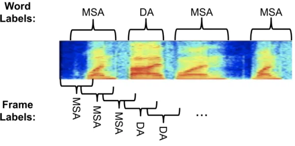
This experiment utilized a simple frame-level binary classification approach. Each MFCC feature frame was matched with a binary label based on if the frame occurred during a MSA segment or a DA segment of the utterance. This determination was made using the forced word alignments, a file which provides the starting timestamp and duration of each word in the dataset within its designated audio clip. Frames were assigned a single timestamp based on the start of the frame window. They were then mapped to a word-level binary label generated from the forced word alignments and transcripts. Figure 4-3 visualizes the frame-level label extraction process.

This classification scheme comes with a small level of error, propagated from the error in the generated forced word alignments file. Work conducted by colleagues at QCRI found that this error was largely negligible.

Figure 4-3: Frame-level binary label extraction process. Word-level labels were gen-erated using the transcripts as well as the timestamp and duration information pro-vided by the forced word alignment file. Frames were then mapped to word-level labels based on the start of the frame.

4.2.2

Neural Network Classifier

Two main considerations were taken into account when beginning the binary clas-sification experiment. First, the difficulty of training a large NN, observed in the previous experiments detailed in Section 4.1. Second, the reduced amount of training data. Keeping these factors in mind, we aimed to create a NN classifier with a rela-tively small number of trainable parameters. However, using a standard feed-forward NN to make a frame-level dialect predictions, based on only 25 ms of audio data, seemed impractical. We therefore opted to use a single layer CNN, in order to mini-mize the number of model parameters and provide a contextual window around each frame for use in final classification.

The model consisted of a single convolutional layer with kernel size 25, followed by batch normalization layer, ReLu activation, a linear layer used to map to the binary output size, and finally a LogSoftmax activation to generate class-level log probability values (Figure 4-4). The model was trained using a learning rate of 10−3, NLL loss, and an early stopping regularization technique.

Figure 4-4: NN classifier architecture. The convolutional layer utilizes a kernel size of 25. Final LogSoftmax activation is not shown.

4.2.3

Evaluation and Results

Evaluation was conducted using the held-out test set. Each frame of an utterance was given a binary label (MSA or DA) based on the model output probabilities. These labels were then compared to the ground truth labels obtained from the forced word alignments. Overall accuracy as well as class-level precision, recall, and F1 scores were then calculated at the frame-level. The baseline results were computed by labeling each frame as the majority class in the dataset: MSA. Table 4.7 contains the baseline results.

Class Accuracy Precision Recall F1 MSA

82.6% 0.826 1.0 0.905

DA 0.0 0.0 0.0

Table 4.7: Baseline results for the binary classification experiment. Results were obtained by labeling each frame as MSA, the majority class. Overall accuracy and precision, recall, F1 scores by dialect class are displayed. Calculated at the frame-level using the reduced dataset test set.

to frames, a receiver operating characteristic (ROC) curve was plotted. The DA probability threshold corresponding to the equal error rate operating point was chosen for use. For this model the threshold for classification was:

class =      DA if x ≥ 0.19 M SA otherwise (4.2)

The results using this threshold for classification can be seen in Table 4.8. Class Accuracy Precision Recall F1

MSA

69.8% 0.841 0.782 0.810 DA 0.225 0.301 0.257

Table 4.8: Results for the CNN model using the classification threshold described in (4.2). Overall accuracy and precision, recall, F1 scores by dialect class are displayed. Calculated at the frame-level using the reduced dataset test set.

Upon closer inspection of the DA class probability outputs, it became clear the model was severely biased toward MSA and did not appear to show any indication it had learned differences between MSA and DA. Figure 4-5 shows examples of DA class probability outputs from two different utterances as well as their associated ground truth labelings. As can be seen in the provided examples, the outputs lacked any discernible pattern or similarity linking them to the ground truth labelings.

4.2.4

Conclusions

It is a difficult task to train, classify, and evaluate code-switching data at the frame-level. The frame-level label, itself, does not precisely match the ground-truth tran-scription labels; as is seen in Figure 4-3. A single frame could span two words in differing dialects; however, it will only be given the label of the word that occurs at the beginning of the frame.

Even with the model’s ability to make use of a contextual window of frames for classification, at a low-level the task drifts away from code-switching detection and more closely resembles a very short-input dialect identification task. Unfortunately, without relying on manual annotations or other acoustic systems, it is impossible to

Figure 4-5: Two examples of DA class probability outputs from different utterances as well as their associated ground truth labelings. A value of 1.0 represents the DA class and a value of 0.0 represents the MSA class.

segment the raw audio data at a more natural level. Training at the word-level or di-alect segment-level would both better align with the labels provided in the transcripts and the natural division of language.

Chapter 5

Alignment-Free Code-switching

Detection System

The failures of the systems described in Chapter 4 were, in part, due to their clas-sification schemes. The CMI clasclas-sification method proved to be underspecified and reliant on factors that are difficult for a model to learn. Frame-level binary classi-fication was accompanied with a level of ambiguity and error due to the mapping from labeled word to frame. The alignment-free code-switching detection system uti-lizes word-level granularity and CTC loss to train the NN classifier on variable-timed labels, while still outputting time specific predictions.

5.1

Data Processing

Many experiments were conducted on this system utilizing both the full and reduced datasets. The results from the use of the reduced dataset are more compelling. Thus, the remainder of Chapter 5 will focus on the work completed using this dataset. As before, the dataset was split into separate train, validation, and test sets using a 70/15/15 percentage split.

5.1.1

Feature Extraction

MFCC features were extracted for use as input into this system. Trials were completed using MFCCs with various window sizes, strides, and dimensionality. Consistently the best performing features utilized standard MFCC parameters: 25 ms window, 10 ms stride, dimension 39 including deltas and delta-deltas.

5.1.2

Classification

This system was trained using CTC loss, described in Section 2.2.1. CTC loss training allows the model to output frame-level predictions, but train using a lower granular-ity target label. For this system, word-level target labels were extracted using the transcripts. Each word in the utterance was given a binary label based on if the word occurred during an MSA segment or a DA segment of the utterance. Frame-level labels were also extracted for use in evaluation. Each MFCC feature frame was matched with a binary label based on if the frame occurred during an MSA segment or a DA segment of the utterance. As previously stated, frame-level labels come with a small amount of error due to the mapping between the forced word alignments and the frames.

5.2

Bi-LSTM + Attention Classifier

The NN architecture of this system is composed of a bi-LSTM layer, an attention module, and a final linear layer/LogSoftmax activation to generate log probability values (Figure 5-1).

5.2.1

Bi-LSTM

The bi-LSTM portion of the architecture is made up of a single layer bi-LSTM with hidden dimension 100. The temporal and context-dependent nature of the data lends itself well to the use of a bi-LSTM. This specialized NN is able to utilize contextual information in both the forward and backward direction, allowing each hidden state

Figure 5-1: Bi-LSTM + Attention architecture. In implementation, the hidden di-mension of the bi-LSTM layer, H, is of size 100. Final LogSoftmax activation is not shown.

associated with a frame to take into consideration information from acoustic data occurring before and after it.

5.2.2

Attention Module

Due to the poor results obtained using an attention module in Section 4.1, experiments with a variety of different attention modules were conducted before settling on the module shown in Figure 5-1. These experiments are described in Section 5.5.3.

The addition of an attention module, with a small number of trainable parameters, to the bi-LSTM layer achieved the best results. This attention module makes use of a FC linear layer to map the sequence of hidden states, output by the bi-LSTM, to a single-dimensional attention vector. The values of the attention vector are then scaled to fall between [0, 1]. Element-wise multiplication is then used to apply the

attention vector values to the sequence of hidden states.

5.3

Alignment-Free Training

Training was conducted using CTC loss. CTC loss is useful for training variations of RNNs, such as bi-LSTMs, where the input data is sequential, but the timing of the target labels is variable. A major goal of this work was to construct a model which, after initial training, only requires an audio clip as input; no transcriptions or manual segmentation of any kind. As the model is both meant to be automatic and aid other acoustic systems, it should not rely on additional manually generated input or input from the acoustic systems it should be aiding.

The data from the reduced datset was first artificially segmented into frames, in order to extract features and feed the data into the model. However, training and evaluating at this artificial frame-level does fit the task well. Multiple frames often represent single words or dialect segments - natural forms of utterance segmentations. Due to variable timing, we were unable to partition the raw input data at these more natural segmentation points. However, by utilizing CTC loss and the transcription data at training time, the model was able to take in artificially segmented observations (frame-level) and learn using naturally segmented labels (character-level, word-level, or dialect segment-level). Thus, the model does not require any specific segmentation or transcription data after training; only raw acoustic data.

For this system we chose to train the model using word-level target labels. Character-level target labels caused the output of the model to frequently shift its probability estimates between classes within short timespans. The focus of this task is intra-sentential code-switching, not intra-word code-switching. Thus, frequent shifts in output values such as this are undesirable. Segment-level targets led to issues in the model learning the distribution of MSA and DA in the dataset. Many DA segments are very short when compared to MSA segments; on average they are a quarter of the length of MSA segments (Table 3.2). Using segment-level targets caused the model to lose this valuable information at training time. Training the model at the word-level

greatly reduced the chances of sporadic, noisy outputs as well as allowed the model to view the data at a natural level of segmentation present in any type of speech data. Despite training at the word-level, the model still provides probability estimate outputs at the frame-level.

During initial training runs, gradients often went to infinity due to the inherent numerical instability of CTC loss. Utilization of a smaller learning rate, 10−4, helped to lessen the issue. Any remaining infinite gradients were zeroed out at each back-propagation step. Early stopping regularization, based on the validation loss, was also used in the training of this system.

5.4

Further Processing and Peak Detection

The NN model used in this system outputs frame-level log probabilities for three possible classes: MSA, DA, and blank. The blank label, required for training with CTC loss, is used to represent the lack of a prediction at a time step. Although the blank is important for many tasks, such as ASR, for this task we chose to remove the blank output prediction entirely. After the removal of the blank class probabilities, the log probabilities of the MSA and DA predictions were converted to a linear scale and renormalized. Due to the binary nature of the classification, the two-channel class prediction values encoded redundant data. Thus, the MSA prediction values were discarded in favor of the DA values. This left a single prediction value for each frame. When the prediction value is close to zero the frame is likely MSA; conversely, when the prediction value is close to one the frame is likely DA.

After cleaning, the prediction values produced by this model tended toward zero, likely MSA, with occasional spike-like increases toward one, likely DA. An example output can be seen in Figure 5-2. This general prediction pattern prompted us to view the problem through the lens of the Matrix language-frame model. Slightly modifying the code-switching task to instead detect where DA words and short phrases are inserted into a mainly MSA utterance. This form of short DA segment insertions is common in the reduced dataset.

Figure 5-2: Example DA probability estimates for a single utterance.

Figure 5-3: Filtered DA probability estimates for the same utterance shown in Figure 5-2. Detected peaks are marked in red.

A post-processing methodology of filtering and peak detection, commonly seen in spoken term detection tasks, was utilized to detect likely locations of DA insertions within an utterance. A median filter with kernel size 31 was passed over the predic-tion values. This filter was used to smooth outliers and remove small spikes in the data, which commonly occurred, but did not tend to be representative of true DA detections. An example of the output from Figure 5-2 passed through the median filter can be seen in Figure 5-3.

After filtering the data, peaks in the prediction values were detected by locating local maxima. Specifically, the peak detection was done by comparing the prediction