HAL Id: hal-01779011
https://hal.archives-ouvertes.fr/hal-01779011
Submitted on 26 Apr 2018
HAL is a multi-disciplinary open access archive for the deposit and dissemination of sci-entific research documents, whether they are pub-lished or not. The documents may come from teaching and research institutions in France or abroad, or from public or private research centers.
L’archive ouverte pluridisciplinaire HAL, est destinée au dépôt et à la diffusion de documents scientifiques de niveau recherche, publiés ou non, émanant des établissements d’enseignement et de recherche français ou étrangers, des laboratoires publics ou privés.
To cite this version:
R. Koech, B. Molle, A. Pires de Camargo, P. Dimaiolo, M. Audouard, et al.. Intercomparison drip-per testing within the INITL. Flow Measurement and Instrumentation, Elsevier, 2015, 46, pp.1-11. �10.1016/j.flowmeasinst.2015.08.003�. �hal-01779011�
Intercomparison dripper testing within the INITL
Richard Koech1*, Bruno Molle², Antonio Pires de Camargo³, Pascal Dimaiolo², Mathieu Audouard², Ezequiel Saretta³, José Antônio Frizzone³, David Pezzaniti4. Gao Benhu5.
1
School of Environmental and Rural Science, University of New England, Armidale NSW 2351, Australia.
²National Research Institute of Science and Technology for Environment and Agriculture, Montpellier, France.
³National Institute of Science and Technology in Irrigation Engineering, Piracicaba-SP, Brazil.
4
Australian Irrigation and Hydraulic Technology Centre, University of South Australia, PO Box 2471, Adelaide, Australia.
5
China Institute of Water Resources and Hydropower Research. *Corresponding author, email: [email protected]
Abstract
The International Network of Irrigation Testing Laboratories (INITL) undertook a laboratory intercomparison testing exercise of three sets of drippers in the period 2013 and 2014. The four testing facilities that participated in this exercise are based in following countries: Australia, Brazil, France and China. The objective of the testing program was to compare results from different independent testing facilities to enable individual laboratories identify potential opportunities for improvement of their performances. This would also facilitate the INITL to make proposals for harmonisation of the testing methods. The maximum coefficient of variation, cv, at the manufacturer’s recommended
operating pressure of 100 kPa, was found to be 3.76 %, which was significantly smaller than the 7% recommended by ISO 9261 (2004) as the maximum allowable variation of the flow rate of the test sample. The emitter exponent was determined to be approximately 0.5 which is consistent with results obtained from past studies. At the operating pressure of 100 kPa, it was found that although the average flow rates from the participating laboratories were similar, there was a difference in the dispersion of data. Datasets for the 4 L h-1 dripper model fitted a normal distribution model, while on the other hand, some datasets for the 2 and 8 L h-1 dripper models were not normally distributed. A higher dispersion of measurements can be interpreted as a higher instability of the testing conditions. The variance for the 2 L h-1 dripper model was found to be homogeneous, while non-homogeneous for the other two models. The latter implies that at least one of the laboratories presented an uncertainty of measurement significantly different from the others. The measurement uncertainty undertaken in this study demonstrated that there were opportunities to improve the measurement process. Recommendations and suggestions for harmonisation of test procedures and improvements in individual laboratories are also identified in this paper.
Nomenclature
INITL International Network of Irrigation Testing Laboratories ISO International Standards Organisation
IEC International Electrotechnical Commission NATA National Association of Testing Australia
Cgcre General Coordination for Accreditation of the National Institute of Metrology, Quality and Technology
cv Coefficient of variation (%)
Mean of sample
sq Standard deviation of the sample
q Flow rate (L h-1)
Q Flow rate (m3 s-1)
m Mass (kg)
t Test duration (s)
ρ Density of water (kg m-3)
T Temperature of pure water (°C)
k Emitter constant
p Emitter inlet pressure (kPa)
m Emitter discharge exponent
i 1, 2, 3, ……n
n Number of measurements/observations AIHTC Australian Irrigation and Technology Centre
IWHR China Institute of Water Resources and Hydropower Research CNAS National Accreditation Service for Conformity Assessment ILAC International Laboratory Accreditation Cooperation
INCT-EI National Institute of Science and Technology in Irrigation Engineering ESALQ/USP Luiz de Queiroz College of Agriculture
IRSTEA National Research Institute of Science and Technology for Environment
V Volume of water in the collector (m3)
Cc Calibration uncertainty Cd Drift uncertainty Cr Resolution uncertainty Ct Temperature uncertainty Cp Pressure uncertainty Cs Salinity uncertainty
Cswr Stop-watch resolution uncertainty
Ctt Test time uncertainty
Ce Uncertainty in evaporation
Cb Uncertainty as a result of buoyancy effect
Ui Raw uncertainty estimate
Estimated semi-range of a component of uncertainty associated with an input estimate
ki Reducing factor associated with an input quantity
vi Degrees of freedom
u(xi) Standard uncertainty (u) of an input quantity (xi)
ci Sensitivity coefficient
uc Combined standard uncertainty
U Expanded uncertainty
kc Coverage factor
veff Effective number of degrees of freedom
1. Introduction
Agriculture is by far the largest consumer of fresh water, and contributes to approximately 70 % of all withdrawals annually on a global scale. However, with the increasing human population, it is facing competition for the scarce water resources from domestic and industrial users. There is therefore a recognised need to undertake research on efficient methods of utilising the scarce water resources. Testing and validation of irrigation equipment performance is seen as a key aspect in improving water use efficiency worldwide.
On the other hand, the world has increasingly become a global market with various commodities and equipment, including irrigation equipment, being manufactured and sometimes tested by independent bodies in one part of the world and marketed globally. To gain international recognition and acceptance in this competitive environment, there is therefore a need for testing facilities and laboratories to demonstrate competence by benchmarking their performance with their peers in the rest of the world.
The INITL is a network of 18 testing laboratories involved in testing of irrigation equipment. The laboratories are spread out in 17 countries in six continents, four of which participated in the latest round of testing drippers. The network promotes initiatives aimed at improving water management and savings through the testing and validation of the performance of irrigation products, with inter-laboratory tests being one of its flagship projects.
In the wider field of metrology, intercomparison testing exercises are commonly practised both nationally and internationally. In Australia for instance, testing facilities accredited to the National Association of Testing Australia (NATA) are required to participate in an intercomparison testing program, better known as the proficiency testing program, to maintain their accreditation or when requesting extension of their scope of accreditation. Similarly, in Brazil, the General Coordination for Accreditation of the National Institute of Metrology, Quality and Technology (Cgcre), the accreditation body recognised by the Brazilian Government, requires that laboratories with accredited tests present proficiency testing results every four years to maintain their accreditation. Proficiency testing is basically a comparison exercise of results of the same products obtained from different facilities. Through participation in proficiency testing, facilities are able to verify their methods and testing procedures, identify potential problems with their testing and generally improve the standard of their testing.
As mentioned above, with the dwindling water resources available for irrigation, a lot of emphasis has been directed towards encouraging water-efficient application methods. The drip system is widely seen as both water and labour efficient, and has consequently witnessed rapid developments and expansion in the recent past. On a global scale, the area of land under drip irrigation increased by approximately 5 million hectares between 1986 and 2006 (Reinders 2006).
In line with the worldwide expansion of the drip system, a significant number of drip systems have entered the market. This necessitated a review of the dripper testing protocols in order to keep up with the rapid changes in technology. The main objective of the first INITL dripper testing program undertaken in 2005-2007, whose results have not been published, was to collate data and information to be used for the revision of the International Standards Organisation (ISO) 9261. This also acted as a baseline worldwide survey of the performance of the leading facilities involved in testing irrigation
equipment. Between 2013 and 2014, a second dripper intercomparison testing was undertaken with the major aim of comparing dripper test results from different independent testing facilities to enable individual facilities to identify opportunities for improvement of their performances. A number of laboratories were also required to participate in the exercise for certification purposes. The two rounds of the testing exercises each involved the use of three sets of dripper specimens (of 25 drippers per set).
This paper reports the results of the second round of dripper intercomparison exercises. An uncertainty analysis was undertaken to identify potential sources of error and opportunities for improvement of the measurement process. Based on these results, recommendations on how to harmonise testing methods and improve testing performances in individual laboratories are suggested.
2. Hydraulics of drip systems
Drippers are outlets used for supplying water in small amounts to the soil for plant growth in drip (or trickle) irrigation systems. They can be categorised as either online or inline drippers. Online drippers are attached to the lateral while inline drippers are integrated into the laterals during manufacturing. Drippers can also be categorised as pressure regulating and non-pressure regulating. Pressure regulating drippers are designed to discharge at constant flow rates over a wide range of operating pressure, while flow rates vary according to pressure in non-pressure regulating drippers.
A range of factors are considered in the design of a drip irrigation system including the operating pressure, frictional losses, size and length of the lateral and water temperature. As opposed to the sprinkler and other systems of irrigation where water is spread over the entire farm, drippers supply water directly to small areas in the vicinity of the plant roots at low flow rates (typically 0.5 - 20 litres/hour). Therefore, in drip systems it is vital that all drippers are working and that water is uniformly distributed. The uniformity of flow in a drip system is affected by the hydraulic design, manufacturer’s variation in the design of emitters and emitter spacings (Wu, 1997). The significance of the influence of the manufacturer’s preciseness is attributed to the fact that emitter flow paths are small (typically less than 2 mm in diameter), and therefore a small deviation in diameter would result in relatively large deviations in discharge (Karmeli, 1977). The drip system is often seen as more water and labour-efficient as compared to other methods of irrigation.
The ISO 9261 (2004) recommends the use of the cv to determine the uniformity of flow or emission
rates of a sample (25) of drippers. This requires the determination of average flow rate ( ) and the standard deviation (sq) of the sample. The cv (%) of the sample is calculated as follows:
= 100 (1)
Emitters may also be characterised by the determination of flow rate as a function of inlet pressure and the emitter constant and exponent. Flow rate-inlet pressure curves are obtained by determining the average flow rate (of the 25 emitters) at each pressure level and plotting these against the inlet pressure. The relationship between flow rate, q, and inlet pressure in the emitter, p, can be characterised by the generalised orifice equation of the form:
= (2)
where k is a constant and m is the emitting discharge exponent. Using the values of flow rates q and their corresponding inlet pressure p, the ISO 9261 (2004) recommends the use of the least square
method to determine the coefficient k and exponent m. It is obvious from Eqn. 2 that the higher the value of exponent m, the more will the flow rate q be affected by pressure, and vice versa. The value of the exponent m for pressure and non-pressure compensating orifice and nozzle emitters is approximately 0 and 0.5, respectively (Karmeli, 1977). The constant, k, is a function of the size of opening and its characteristics.
3. The intercomparison testing exercise
3.1 INITL Testing facilities
Information about the testing laboratories that participated in the 2013-2014 dripper intercomparison tests may be accessed from their corresponding websites:
(1) AIHTC – Australia: http://www.unisa.edu.au/Research/CWMR/AIHTF/ (2) IWHR – China: http://www.iwhr.com/
(3) INCT-EI – Brazil: http://www.esalq.usp.br/inctei/ (4) IRSTEA – France: http://www.irstea.fr/
3.2 Testing procedure
Model E1000 drippers manufactured by John Deere were used in the intercomparison exercise. Three sets each of 25 online, non-pressure compensating drippers were used with the following nominal flow rates: 2, 4 and 8 L h-1 and recommended operating pressure of 100 kPa. This model of drippers had been used by some of the co-authors in a previous study (Camargo et al., 2013), and had proved to have a very good level of manufacturing cv. With three sets of drippers and nine pressure levels,
each test facility performed a total of 27 tests (no repetitions). The same online drippers were tested in France, Brazil, China and Australia.
The intercomparison tests were conducted in accordance with the International Standard ISO 9261 (2004). Among other things, this standard provides guidance on emitter test specimens and conditions, as well as test methods and requirements. The specific test procedures designed and adopted by testing facilities are required to conform to the general requirements of the standard. There were slight differences among the test procedures developed and used by each laboratory. The ISO 9261 requirements and the laboratory-specific procedures are discussed below.
3.2.1 General test requirements
The tests were conducted at ambient air temperature and a water temperature of 23 °C ± 3 °C. The standard specifies three categories of tests to be undertaken: (i) uniformity of flow rate; (ii) flow rate as a function of inlet pressure; and (iii) determination of emitter/emitting unit exponent. The uniformity of flow rate is a hydraulic test in which the flow rate of emitters is measured at a single pressure corresponding to the emitter’s operating pressure recommended by the manufacturer, which was 100 kPa in these experiments. It is worth noting that the standard neither specifies how the flow rate is to be measured nor recommendations related to the testing facility design.
To determine the relationship between the flow rate and the inlet pressure, the standard requires that the pressure be increased in steps not greater than 50 kPa, from zero up to 1.2 of the maximum pressure. The following nine pressure levels were adopted by all the testing facilities: 80, 100, 120, 140, 160, 180, 200, 220 and 240 kPa. The flow rate was measured for each emitter at these pressure levels. The data was also used to determine the emitter constant and exponent.
3.2.2 Laboratory-specific test procedures
AIHTC (Australia)
The test rig used at the AIHTC consisted of the following major components: a water reservoir, a pump, 40 mm manifold and 15 cm long pipes of 12 mm nominal diameter attached to either side of the manifold. A close mesh metal bar grating was used to cover the reservoir, which also acts as a platform on which the one-litre plastic collectors used to collect water from each emitter were placed. The drippers, spaced at 30 cm, were attached to the 12 mm nominal diameter pipes.
Generally for all the tests, the measurement system was conditioned for approximately one hour by starting the pump and running the water through the pipe network and the drippers. Testing was commenced while the pump was still running, by sequentially (after about every 5 seconds) placing a collector on the platform directly under each emitter. At the end of the each test, the same order was used in removing the collectors from the test rig. Due to the capacity of the collectors used and the drippers’ flow rate, the test duration for all tests was approximately 5 minutes.
The inlet pressure, water temperature and salinity, and ambient temperature were measured for each test. The evaporative loss was determined using a one-litre collector half-filled with water and placed in the vicinity of the test rig. The difference between the initial and the final reading (corresponding to the start and end of the each test) of the collector was assumed to be the mass of water lost due to evaporation, and was thus added to the net mass of water collected.
The mass of water in each collector was determined using a measuring scale immediately they were removed from the test rig, but after wiping the water on the outside of the collectors using a dry piece of cloth. The flow rate, Q (m3 s-1), of each emitter was determined as follows:
= (3)
where m (kg) is the mass of water in each collector, ρ (kg m-3) is the density of water and t (seconds) is the test duration. The density of water in Eqn. 3 was corrected for temperature (Fig. 11.1.1 in McCutcheon et al., 1993), pressure (NMI 2004) and salinity (Eqn. 11.1.2 in McCutcheon et al., 1993), which are the main factors affecting density of water in testing facilities.
IWHR (China)
The test bench used to undertake the tests at the IWHR was fully automated. It consisted of 25 automatic water collecting and weighing devices, corresponding to each of the 25 emitters tested. The maximum capacity of each collector was 1.5 L, and the resolution of the measuring device was 0.1 g. A motor controller was used to automatically control the operation of the water pump. The inlet pressure was measured using a pressure transducer with a range of 10 - 800 kPa and a resolution of 0.1 kPa. The water used for the test was drawn from a 800 L stainless steel tank. The water level in the tank remained constant throughout tests. The temperature of the water was automatically controlled using a heating and cooling system with a resolution of 1 °C, while the accuracy of the automatic timer used was 0.01s. The test bench was connected to a central automatic control and data processing system.
INCT-EI (Brazil)
The bench used to perform the tests has the following major components: 300 L water tank; water pump equipped with a variable-frequency drive and Proportional-Integral-Derivative (PID) controller
to set and automatically maintain the testing pressure; 4 L plastic collectors for collecting water from each of the 25 emitters monitored; precision measuring scale; stopwatch; and thermo-hygrometer. The flow rate of each emitter is determined based on the mass of water collected at the end of the test. The testing bench has a movable platform, on which the collectors are placed, that enables all the 25 collectors to be moved instantaneously at the beginning and at the end of the test. The water and air temperatures are monitored, controlled and recorded during the tests. The air humidity is also monitored and recorded. Evaporative losses are assumed to be negligible since within the laboratory there is neither wind nor insolation, the air temperature is controlled, and air humidity remains relatively high during tests (>50%). At the end of the tests, the mass in the collectors is weighed by a precision scale after wiping the external walls of the collectors with a dry piece of cloth to remove droplets of water. The flow rate of each emitter is calculated using Eqn. 3. However, in this case the water density, ρ, is corrected according to the average water temperature (T) during the test (Eqn. 4).
= −0.00361 − 0.06383 + 1000.4342 (4)
Eqn. 4 was obtained by fitting an equation to water density data at various temperatures. The duration of the tests was 30 minutes for the 2 and 4 L h-1 dripper models, and 20 minutes for the 8 L h-1dripper model.
IRSTEA (France)
The facility is supplied from a 1 m3 water tank, with the temperature controlled at 23°C and the pressure regulated by an automatic pneumatic valve. It constitutes of a series of collecting tubes of constant section. In each tube the height of the water column is measured by a pressure transducer connected to its bottom. The discharge is adjusted statistically from successive measurements of this height at 1 second time steps. The discharge is considered steady when the regression coefficient of the successive measurement overpasses 0.999. This avoids errors related to time evaluation and reduced possible variations due to the fluctuations of pressure in the supply system.
4. Evaluation of data
4.1 Statistical analysis
The study reported in this paper involved three sets of online drippers with 25 drippers per set, and tests were performed over nine pressure levels (total of 27 tests). A range of statistical analyses were undertaken on the data obtained from the participating laboratories using the software IBM SPSS Statistics (Version 22). The Kolmogorov-Smirnov’s test was used to test the normality of flow rate provided by each laboratory. All the statistical tests were performed assuming 95% confidence interval.
An evaluation was undertaken to test if the dispersion or variability of flow rate differed considerably among the participating laboratories. A statistical analysis was performed to test the homogeneity of variances in flow rates reported by the participating laboratories. The aim of this statistical procedure was to establish the similarity or otherwise of the variability of flow rates among the laboratories. Since the same drippers were tested by all the laboratories and assuming that the drippers did not suffer any change in its characteristics, the lower the variability (variance, standard deviation) of flow rate, the lower the uncertainty of the test performed by a given laboratory. The assumption effectively ignores the Mullins’ effect (Mullins, 1947; Diani et al., 2009), which suggests that the mechanical
properties of rubber-like materials (for instance drippers) may change due to some transitory elastic phenomenon.
Therefore, the statistical analysis aimed to ascertain if the four laboratories were able to provide similar results in terms of variability of flow rate. Bartlett’s and Levene’s tests were used to assess the homogeneity of variances for the variable flow rate among the four laboratories. Bartlett's test is sensitive to departures from normality, which means that the set of data from each laboratory must follow the normal distribution curve for this model to be applied. This test was used to analyse the 4 L h-1 model of drippers, whose average flow rates in all the four laboratories were found to be normally distributed. On the other hand, Levene’s test is less sensitive than the Bartlett’s test to departures from normality and can be used when the set of data from one or more laboratories do not follow the normal distribution. This test was subsequently used to analyse the 2 and 8 L h-1 dripper models.
4.2 Uncertainty analysis
The uncertainty is a parameter that characterises the dispersion of values and may be obtained by a Type A or B evaluation, but both types of evaluation are based on probability distributions, and the uncertainty components resulting from either type are quantified by variances or standard deviations (JCGM, 2008). Type A uncertainty estimates are obtained from statistical treatment of repeated measurement results and are usually associated with random errors. On the other hand, type B uncertainty estimates are obtained without the use of repeated measurements and usually are related to systematic errors. In metrological facilities, measurement uncertainties are quantified in order to understand the quality of measurement and to allow objective comparison with results from different laboratories.
Uncertainty analysis is specific to the particular test procedure applied and the set of equipment used, and hence each of the participating laboratories has its own method. However, the general metrological principles are the same. To illustrate the process and to demonstrate how it can be used to identify opportunities for improvement of the measurement process, the methodology developed by one of the participating laboratories (AIHTC) will be used. The procedure is described by Bentley (2005) and may be summarised into the following key steps: modelling of the measurement; listing of all error sources; characterisation of all error components; determination of the standard uncertainty for the measurement; determination of the combined standard uncertainty; calculation of the expanded uncertainty; and statement of the results.
In this study, the measurand was assumed to be the flow rate, Q, derived from measurements of volume of water collected in the collector, V, and the test time, t. However, the volume was not measured directly; it was inferred from the measurement of mass, m. Hence the model for the determination of the measurement uncertainty may be represented by Eqn. 3 above. Sources of error that could potentially affect the measurements are described in Section 5.3.
For an input quantity determined from n independent repeated observations, the standard uncertainty is expressed by the experimental standard deviation of the mean, !, according to Eqn. 5, and is called Type A standard uncertainty.
where " ! is the standard uncertainty of an input quantity ; is the standard deviation of n individual observations.
Type B evaluations of uncertainty require a knowledge of the probability distribution associated with the uncertainty. The most common symmetrical distributions are rectangular, normal, triangular, and bimodal (ISO 5168, 2005). In these cases, " ! is calculated according to Eqn. 6.
" ! =&'
(' (6)
Where: is the estimated semi-range of a component of uncertainty associated with an input estimate; is the reducing or coverage factor. A typical Type B evaluation occurs when the calibration certificate gives the expanded uncertainty (U) of a measurement instrument. In this situation, the value of corresponds to U and the value of also comes from the calibration certificate.
Once the standard uncertainties of the input quantities and their corresponding sensitivity coefficients have been determined from either Type A or Type B evaluations, the combined uncertainty of the output quantity, ") *!, can be determined according to Eqn. 7:
") *! = +∑ - " !./01 (7)
where: N is the number of input quantities on which the measurand depends; is the sensitivity coefficient associated to each of the input quantities. A sensitivity coefficient describes how the output estimate y varies with changes in the values of a given input quantity ( ) and it can be determined by an analytical or numerical solution, as shown in Eqn. 8 (ISO 5168, 2005).
=2423'≈∆4∆3' (8)
The combined standard uncertainty (")) factors in the standard uncertainty of each input quantity resulting in a single value that has a confidence level about 68%. Such confidence level is not enough in engineering applications that usually require uncertainty statement with 95% confidence level. The coverage factor ( )) is a numerical value used as a multiplier of the combined standard uncertainty in order to obtain the expanded uncertainty (JCGM, 2008), and it is dependent on characteristics of the error distribution. Statistically, degrees of freedom are the number of independent comparisons that can be made among the elements of a sample (Montgomery and Runger, 2011).
The number of degrees of freedom (vi) is equal to n – 1 for a single quantity estimated by the
arithmetic mean of n independent observations, and it occurs in most cases related to Type A uncertainties. For Type B uncertainties, assigning infinite degrees of freedom is realistic considering that it is a common practice to choose lower and upper limits of an input quantity ( 7 and 8, respectively) in such a way that the probability of the quantity in question lying outside the interval
7 to 8 is extremely small (JCGM, 2008). On the other hand, Bentley (2005) suggests the use of four values of vi for type B components on the basis of qualitative judgement: 3 (rough), 10
(reasonable), 30 (good) or 100 (excellent).
To determine ), the effective number of degrees of freedom, veff, for the combined standard
uncertainty (uc) has to be estimated (this uses the number of degrees of freedom vi for each component
9:;; =∑A |)'.< 4<=> '!|>/ '
'BC (9)
Using the value of veff calculated in Eqn. 9, the coverage factor kc may be obtained from ‘Student’s t’
table (Table G.2 in JCGM, 2008 or Table 2.2 in Bentley, 2005).
Finally, the combined uncertainty (")) is multiplied by a coverage factor ( )) to obtain the expanded uncertainty (D), as shown in Eqn. 10.
D = ) ") (10)
The uncertainty calculations were undertaken using Excel spreadsheets and the results summarised in Tables 5 and 6, and Fig. 6.
5. Results and discussion
5.1 Flow rate uniformity of emitters
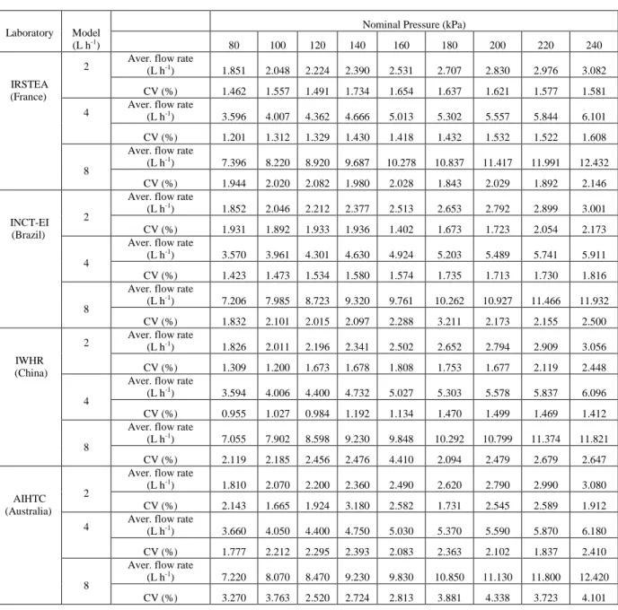
Table 1 summarises the results (average flow rates from the 25 emitters and the cv) obtained from tests
undertaken in the four laboratories that participated in the intercomparison tests. The maximum value of cv in the table is 3.18, 2.41 and 4.41% for the 2, 4 and 8 L h
-1
dripper model respectively. Overall, the cv appeared to increase with the increase in the test pressure. On average, the 4 and the 8 L h
-1
dripper model had the smallest and the largest variation respectively.
There were only minor differences between the average flow rates among the participating laboratories; the differences increasing slightly with the increase in the dripper rating. For instance, at the manufacturer’s recommended operating pressure of 100 kPa, the absolute difference between the highest and the lowest average flow rate was 0.059, 0.089 and 0.318 L h-1 for the 2, 4 and 8 L h-1 dripper model respectively.
Table 1 - Summary of results from four laboratories
Laboratory
Model (L h-1)
Nominal Pressure (kPa)
80 100 120 140 160 180 200 220 240 IRSTEA (France) 2
Aver. flow rate
(L h-1) 1.851 2.048 2.224 2.390 2.531 2.707 2.830 2.976 3.082
CV (%) 1.462 1.557 1.491 1.734 1.654 1.637 1.621 1.577 1.581 4
Aver. flow rate
(L h-1) 3.596 4.007 4.362 4.666 5.013 5.302 5.557 5.844 6.101
CV (%) 1.201 1.312 1.329 1.430 1.418 1.432 1.532 1.522 1.608
8
Aver. flow rate
(L h-1) 7.396 8.220 8.920 9.687 10.278 10.837 11.417 11.991 12.432 CV (%) 1.944 2.020 2.082 1.980 2.028 1.843 2.029 1.892 2.146 INCT-EI (Brazil) 2
Aver. flow rate
(L h-1) 1.852 2.046 2.212 2.377 2.513 2.653 2.792 2.899 3.001
CV (%) 1.931 1.892 1.933 1.936 1.402 1.673 1.723 2.054 2.173
4
Aver. flow rate
(L h-1) 3.570 3.961 4.301 4.630 4.924 5.203 5.489 5.741 5.911
CV (%) 1.423 1.473 1.534 1.580 1.574 1.735 1.713 1.730 1.816
8
Aver. flow rate
(L h-1) 7.206 7.985 8.723 9.320 9.761 10.262 10.927 11.466 11.932 CV (%) 1.832 2.101 2.015 2.097 2.288 3.211 2.173 2.155 2.500 IWHR (China) 2
Aver. flow rate
(L h-1) 1.826 2.011 2.196 2.341 2.502 2.652 2.794 2.909 3.056 CV (%) 1.309 1.200 1.673 1.678 1.808 1.753 1.677 2.119 2.448
4
Aver. flow rate
(L h-1) 3.594 4.006 4.400 4.732 5.027 5.303 5.578 5.837 6.096
CV (%) 0.955 1.027 0.984 1.192 1.134 1.470 1.499 1.469 1.412
8
Aver. flow rate
(L h-1) 7.055 7.902 8.598 9.230 9.848 10.292 10.799 11.374 11.821 CV (%) 2.119 2.185 2.456 2.476 4.410 2.094 2.479 2.679 2.647 AIHTC (Australia) 2
Aver. flow rate
(L h-1) 1.810 2.070 2.200 2.360 2.490 2.620 2.790 2.990 3.080
CV (%) 2.143 1.665 1.924 3.180 2.582 1.731 2.545 2.589 1.912 4
Aver. flow rate
(L h-1) 3.660 4.050 4.400 4.750 5.030 5.370 5.590 5.870 6.180
CV (%) 1.777 2.212 2.295 2.393 2.083 2.363 2.102 1.837 2.410
8
Aver. flow rate
(L h-1) 7.220 8.070 8.470 9.230 9.830 10.850 11.130 11.800 12.420
CV (%) 3.270 3.763 2.520 2.724 2.813 3.881 4.338 3.723 4.101
The AIHTC obtained the largest cv for both the 4 and 8 L h
-1
Models, and the second largest in the case of the 2 L h-1 Model. The IWHR recorded the smallest cv in the case of the 2 and 4 L h
-1
models. The maximum cv of 3.76% was still way below 7% which is recommended by ISO 9261 (2004) as the
maximum allowable variation of the flow rate of the test sample.
In fact, the variability of flow rate, as expressed by the cv, is accounted for by two sources. The first is
the inherent differences among sample of drippers caused by the manufacturing process. The second source is related to the instability of the control and measurement systems employed to perform the tests. For instance, if a system in charge of controlling the testing pressure presents instabilities during the test, the measured flow rates will also reproduce these variations resulting in an increase in dispersion of values and consequently an increase in cv. Theoretically, since the same emitters were
tested by the four laboratories and assuming that their characteristics did not change as the tests progressed from one laboratory to the other, the cv was expected to be similar. Therefore, for a given
sample of drippers of constant characteristics, the differences in variability in flow rate observed among the laboratories represent different degrees of instabilities (uncertainty) of the test performed by each laboratory.
The data obtained from the tests for determining the uniformity of flow rate of drippers are presented in Fig. 1. Box plots are a convenient way of graphically depicting groups of numerical data that indicate the degree of dispersion and skewness in the data, including outliers. Looking at Fig. 1, it seems that the average flow rates are similar in all tests but the dispersion of data seems to be higher in INCT-EI (Brazil) for the emitter model 2 L h-1 as well as in AIHTC (Australia) for the emitter models of 4 and 8 L h-1. Comparing data from the four laboratories, a higher dispersion of measurements can be interpreted as a higher instability of the testing conditions, assuming the drippers did not suffer any change from their initial characteristics. However, additional statistical analysis is required to ascertain if the variability in flow rates was significantly different among the laboratories.
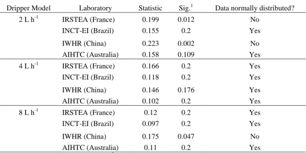
Kolmogorov-Smirnov’s test was used to verify the normality of data provided by each laboratory (Table 2). The dataset for the 4 L h-1 model (from all four laboratories) dripper were found to be normally distributed. However, for the 2 and 8 L h-1 dripper model, data from some laboratories were found not to be normally distributed.
Examples of datasets that do not follow the normal distribution pattern are mentioned by Rocha et al. (2014), who described experiments for determining head loss along polyethylene pipes and found that the operating pressure and head loss of some groups of data did not follow the normal distribution. The international standard ISO/TR 22971 (2005) which describes how to plan and analyse results of interlaboratory comparison tests, recommends that when not normally distributed data is detected, the statistical methods to analyse results must be properly chosen to avoid errors.
(L h -1 ) (L h -1 ) (L h -1) 8 L h-1 4 L h-1 2 L h-1
Fig. 1 - Uniformity of flow rate tests at the operating nominal pressure 100 kPa. [The horizontal line within the box represents the median; the star represents the average; the bottom and top of the box are the lower and upper quartiles; the whiskers represent the maximum and minimum values, excluding outliers; and the dot beyond the whiskers represents an outlier].
Table 2 - Results of Kolmogorov-Smirnov’s test used for assessing the normality of groups of data
Dripper Model Laboratory Statistic Sig.1 Data normally distributed? 2 L h-1 IRSTEA (France) 0.199 0.012 No
INCT-EI (Brazil) 0.155 0.2 Yes IWHR (China) 0.223 0.002 No AIHTC (Australia) 0.158 0.109 Yes 4 L h-1 IRSTEA (France) 0.166 0.2 Yes INCT-EI (Brazil) 0.118 0.2 Yes IWHR (China) 0.146 0.176 Yes AIHTC (Australia) 0.102 0.2 Yes 8 L h-1 IRSTEA (France) 0.12 0.2 Yes INCT-EI (Brazil) 0.097 0.2 Yes IWHR (China) 0.175 0.047 No AIHTC (Australia) 0.11 0.2 Yes
1Sig. > 0.05 for normally distributed data
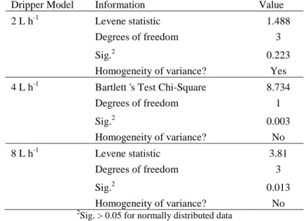
In this study, the assessment of normality is required to choose the statistical test to assess the homogeneity of variances among the datasets. Bartlett’s test was used for assessing the homogeneity of variances of 4 L h-1 drippers, whose data was found to be normally distributed among all four laboratories, while Levene’s test was employed for evaluating the other two models of drippers (Table 3).
Table 3 - Statistical results from the tests to assess the homogeneity of variances at operating pressure of 100 kPa
Dripper Model Information Value 2 L h-1 Levene statistic 1.488
Degrees of freedom 3
Sig.2 0.223
Homogeneity of variance? Yes 4 L h-1 Bartlett 's Test Chi-Square 8.734
Degrees of freedom 1 Sig.2 0.003 Homogeneity of variance? No 8 L h-1 Levene statistic 3.81 Degrees of freedom 3 Sig.2 0.013 Homogeneity of variance? No 2
Sig. > 0.05 for normally distributed data
Observing the results of the 2 L h-1 model dripper (Table 3), the variances of flow rate were statistically equal among the laboratories. That is, the facilities, testing methods, control and measurement systems were able to provide equivalent results in terms of variability of flow rate around the values of 2 L h-1 and consequently the uncertainty of measurement is probably similar among the laboratories. On the other hand, the variances of flow rate were different among the laboratories in the case of the other two models. This implies that the laboratories were not able to provide equivalent results in terms of variability of flow rate. That is, for flow rates around 4 and 8 L h-1, at least one of the laboratories presented an uncertainty of measurement significantly different from the others.
As implied above, the differences in the dispersion of data among the participating laboratories points to differences in their measurement accuracies. This is a factor of the specific measurement procedures and equipment used. Improvement in the accuracy of the measurement process can be attained by a critical analysis of all the factors that could potentially affect the measurement. This is explored further in section 5.3 of this paper.
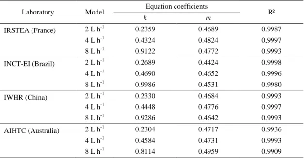
5.2 Flow-inlet pressure curves and the emitter constant and exponent
The emitter exponents (m) and constants (k) are shown in Table 4. The table shows that the emitter exponent obtained at the four laboratories was approximately 0.5 for all three sets of drippers, with a maximum absolute deviation of 0.0428 for the 8 L h-1 model. This magnitude of exponent is consistent with results reported by Karmeli (1977). The absolute deviation of the values of constant (k) for the 8 L h-1 model was 0.1872.
Table 4 - Determination of emitter constant (k) and exponent (m)
Laboratory Model Equation coefficients R²
k m IRSTEA (France) 2 L h-1 0.2359 0.4689 0.9987 4 L h-1 0.4324 0.4824 0,9997 8 L h-1 0.9122 0.4772 0.9993 INCT-EI (Brazil) 2 L h-1 0.2689 0.4424 0.9998 4 L h-1 0.4690 0.4652 0.9996 8 L h-1 0.9986 0.4531 0.9980 IWHR (China) 2 L h-1 0.2330 0.4684 0.9993 4 L h-1 0.4448 0.4776 0.9997 8 L h-1 0.9286 0.4642 0.9993 AIHTC (Australia) 2 L h-1 0.2304 0.4717 0.9936 4 L h-1 0.4584 0.4731 0.9993 8 L h-1 0.8114 0.4959 0.9909
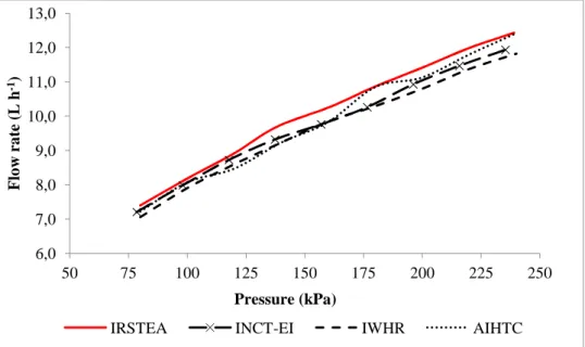
The flow rate-inlet pressure relationships are depicted in Figs. 2, 3 and 4 for the 2, 4 and 8 L h-1 dripper models respectively. The graphs show that there were only minor differences between the laboratories (particularly for the 8 L h-1 model). This further reinforces the conclusion arrived at above that the results obtained from the participating laboratories are highly comparable.
Fig. 2 - Comparison of flow rate as a function of pressure (Model 2 L h-1)
1,5 2,0 2,5 3,0 3,5 50 75 100 125 150 175 200 225 250 F lo w r a te ( L h -1) Pressure (kPa) IRSTEA INCT-EI IWHR AIHTC Puissance (AIHTC)
Fig. 3 - Comparison of flow rate as a function of pressure (Model 4 L h-1)
Fig. 4 - Comparison of flow rate as a function of pressure (model 8 L h-1)
5.3 Uncertainty budget
The results of the calculations used to determine the measurement uncertainties will now be enumerated; and Tables 5 and 6 is used to illustrate the process. The uncertainty was determined in accordance with Bentley (2005), and relate to the tests undertaken specifically by the AIHTC as explained earlier.
The sources of error that could potentially affect the measurements are: calibration, drift and resolution of the measuring scale, correction of water density for uncertainty in temperature and salinity, stop watch resolution, test time error, uncertainty in evaporation loss, correction for buoyancy (air displaced from collector) and uncertainty due to error in pressure.
y = 0,4584x0,4731 R² = 0,9993 3,0 3,5 4,0 4,5 5,0 5,5 6,0 6,5 50 75 100 125 150 175 200 225 250 F lo w r a te ( L h -1) Pressure (kPa)
IRSTEA INCT-EI IWHR
AIHTC Puissance (AIHTC)
6,0 7,0 8,0 9,0 10,0 11,0 12,0 13,0 50 75 100 125 150 175 200 225 250 F lo w r a te ( L h -1) Pressure (kPa)
Calibration of measuring scale (Cc): The latest calibration report indicated that the uncertainty due to
calibration was 0.5 g (0.0005 kg). The error distribution is normal (ki = 2) and vi = 60 obtained from
the Student’s t table (Bentley, 2005).
Drift of measuring scale (Cd): This was assumed to be half the calibration uncertainty, 0.25 g
(0.00025 kg) and normal distribution (ki = 2). vi was assumed to be 3 (rough estimate) (Bentley,
2005).
Resolution of measuring scale (Cr): The least measurement of the scale is 0.01 g, hence the resolution
is half this least measurement (0.005 g or 0.000005 kg), rectangular distribution (ki = 1.732) was
assumed; vi was assumed to be 100 (excellent estimate) (Bentley, 2005).
Correction of water density for uncertainty in temperature (Ct): Assuming a temperature
measurement accuracy of ±0.4 °C, a variation in density between 29.2°C and 30.0°C represents the maximum density variance due to temperature (variation of ± 0.8 °C assumed). At 29.2°C water density is 995.917 kg m-3 and at 30.0°C water density is 995.678 kg m-3 (calculated using the equation given in Fig. 11.1.1 in McCutcheon et al., 1993). The density difference (0.239 kg m-3) was taken as a correction of water density for uncertainty in temperature. Rectangular distribution was assumed (ki =
1.732) and vi was assumed to be 3 (rough estimate) (Bentley, 2005).
Correction of water density for uncertainty in salinity (Cs): Using data for the 8 L h
-1
dripper model, with measured salinity of 560 µS/cm and temperature of 21.5 °C, the density increase as a result of water salinity was determined to be 0.212 kg m-3 (Eqn. 11.1.2 in McCutcheon et al., 1993). The uncertainty was assumed to be 10 % of this density increase (0.0212 kg m-3). The distribution was assumed to be rectangular distribution (ki = 1.732), and vi was taken to be 3 (rough estimate) (Bentley,
2005).
Stop watch resolution (Cswr): The least reading of the stop watch was 0.01 s, hence the resolution is
0.005 s. The error distribution is rectangular (ki = 1.732). vi was assumed to be 100 (excellent).
Test time error (Ctt): The process of placement and removal of catch cans from the rig (at the start and
end of test respectively), proceeded manually. The placement and removal was undertaken at an interval of approximately 5 seconds, and the uncertainty associated with the test time was about 1 second. The error distribution is rectangular distribution (ki = 1.732) and vi was assumed to be 3
(rough estimate).
Uncertainty in evaporation loss (Ce): The maximum loss due to evaporation measured was about 1 g.
An uncertainty of 10 % was assumed, hence 0.1 g or 0.0001 kg was used in the uncertainty analysis table. Rectangular distribution (ki = 2) and vi of 3 (rough estimate) were assumed (Bentley, 2005).
Correction for buoyancy (Cb): The filling of a catch can involves displacement of air which has a
nominal density of 1.2 kg m-3. The volume of the catch can (diameter 100 mm and height 200 mm) was 0.001571 m3. Hence maximum mass of air displaced is 0.00188 kg. The maximum uncertainty due to buoyancy was assumed to be 10% of the air displaced, that is, 0.000188kg, rectangular error distribution (ki = 1.732) and vi = 3 (rough estimate).
Uncertainty due to error in pressure (cp): According to Zhao et al. (2014), the emitter flow rate
variation due to inlet pressure change, cp (L h
-1
), may be calculated as follows:
where Po is the nominal pressure (kPa); P is the test pressure; k and m are as defined earlier (Eqn. 2).
For the 8 L h-1 dripper model, k = 0.8114 and m = 0.4959 (Table 4). The resolution of the pressure gauge was 0.1 kPa. At a nominal pressure of 240 kPa (Po), the uncertainty in flow rate due to pressure
variation, cp (Eqn. 11), is 0.002 L h
-1
(5.556E-10 m3 s-1). The rectangular error distribution was assumed (ki = 1.732) and vi = 3 (rough estimate).
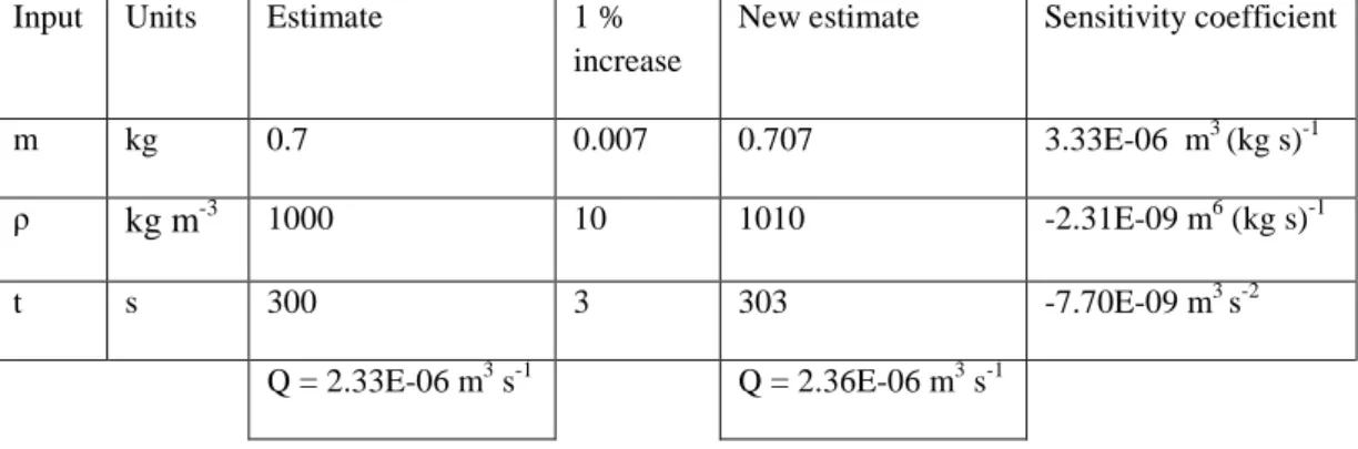
The sensitivity coefficients (Table 5) were calculated numerically using Eqn. 8. The typical data expected for the model (Eqn. 3) and the assumed small increase in the factors are also shown in Table 5.
Table 5 - Sensitivity coefficients
Input Units Estimate 1 % increase
New estimate Sensitivity coefficient
m kg 0.7 0.007 0.707 3.33E-06 m3 (kg s)-1 ρ kg m-3 1000 10 1010 -2.31E-09 m6 (kg s)-1
t s 300 3 303 -7.70E-09 m3 s-2
Q = 2.33E-06 m3 s-1 Q = 2.36E-06 m3 s-1
Table 6 - Uncertainty analysis table
Component Units Distribution Ui ki u(xi) vi ci |ciu(xi)| |ciu(xi)|2 |ciu(xi)|4/vi
Cc kg Normal 5.00E-04 2.000 2.50E-04 60 3.33E-06 8.33E-10 6.94E-19 8.04E-39
Cd kg Normal 2.50E-04 2.000 1.25E-04 3 3.33E-06 4.17E-10 1.74E-19 1.00E-38
Cr kg Rect 5.00E-06 1.732 2.89E-06 100 3.33E-06 9.62E-12 9.26E-23 8.57E-47
Ct kg m-3 Rect 2.39E-01 1.732 1.38E-01 3 -2.31E-09 3.19E-10 1.02E-19 3.44E-39
Cs kg m
-3
Rect 2.12E-02 1.732 1.22E-02 3 -2.31E-09 2.83E-11 8.00E-22 2.13E-43
Cswr s Normal 5.00E-03 1.732 2.89E-03 100 -7.70E-09 2.22E-11 4.94E-22 2.44E-45
Ctt s Rect 1.00E+00 1.732 5.77E-01 3 -7.70E-09 4.45E-09 1.98E-17 1.30E-34
Ce kg Rect 1.00E-04 1.732 5.77E-05 3 3.33E-06 1.92E-10 3.70E-20 4.57E-40
Cb kg Rect 1.88E-04 2.000 9.40E-04 50 3.33E-06 3.13E-10 9.82E-20 1.93E-40
Cp m3 s-1 Rect 5.56E-10 1.732 3.21E-10 3 1.00E+00 3.21E-10 1.03E-19 3.54E-39
Sum 2.10E-17 1.30E-34
Combined standard uncertainty 4.58E-09 Eff degrees of freedom, Veff 3 Coverage factor, k 3.18 Expanded uncertainty(m3 s-1) 1.46E-08 Expanded uncertainty (L s-1) 1.46E-05 Expanded uncertainty (L h-1) 5.25E-02
The expanded uncertainty obtained was 0.0525 L h-1 (Table 6). Hence, as a percentage of the minimum (1.851 L h-1) and maximum (12.42 L h-1) flow rate obtained, the expanded uncertainty would be 2.84 % and 0.42 % respectively. The expanded uncertainty based on average flow rates was determined to be 2.4, 1.1 and 0.6 % for the 2, 4 and 8 L h-1 dripper models respectively.
Fig. 5 (obtained from columns 1 and 9 of Table 6) shows that the uncertainty in the measurement process was dominated by test time error. As explained in the test procedure, the collectors were placed and later retrieved from the test rig manually and hence a relatively high uncertainty over the test time. If an automatic method had been used, with an assumed test time error of zero, the expanded uncertainty would have reduced from 0.0525 to 0.00793 L h-1 (Table 6).
Fig. 5 - Uncertainties in the measurement of flow rate
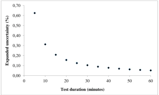
An analysis was undertaken to quantify the effect of the test duration (and therefore the test volume) on the expanded uncertainty using the measurement model assumed in this study (Eqn. 3), the typical estimates of the model shown in Table 5 and the calculated expanded uncertainty (0.0525 L h-1, Table 5). This is illustrated in Fig. 6 shows that the expanded uncertainty reduces with the increase in the duration of the test, as expected. For example, increasing the test duration from 5 to 20 minutes (test time used by INCT-EI for the 8 Lh-1 dripper model), the expanded uncertainty reduced from approximately 0.62 to 0.16 %.
0 10 20 30 40 50 60 70
Calibration of scale Calibration drift Resolution of scale Water density - temperature Water density - salinity Stop watch uncertainty Test time error Uncertainty in evaporation Uncertainty due to buoyancy Uncertainty in pressure
Fig. 6 – Effect of test duration on measurement uncertainty
6. Recommendations and conclusions
Four laboratories participated in the INITL intercomparison dripper testing program undertaken from 2013 to 2014 with the aim of comparing results obtained from similar testing facilities and identifying opportunities for improvements. The maximum cv, at the manufacturer’s recommended operating
pressure of 100 kPa, was 3.76 % which was significantly smaller than the 7% recommended by ISO 9261 (2004) as the maximum allowable variation of the flow rate of the test sample. The emitter exponent was determined to be approximately 0.5 which is consistent with results obtained from past studies.
At the manufacturer’s recommended operating pressure of 100 kPa, using the software IBM SPSS Statistics (Version 22), datasets for the 4 h-1 dripper model fitted a normal distribution model. On the other hand, some datasets for the other two dripper models were not normally distributed. A higher dispersion of measurements can be interpreted as a higher instability of the testing conditions. The variance for the 2 L h-1 dripper model was found to be homogeneous, while non-homogeneous for the other two models. The latter implies that at least one of the laboratories presented an uncertainty of measurement significantly different from the others. Further recommendations and conclusions are enumerated below:
• The reference standard for the dripper tests described in this paper, ISO 9261 (2004), does not specify the details of the method to be used to measure emitter flow rate nor the specifications of the test rig (size/length of laterals/manifold and spacing of drippers among other things). Hence different testing laboratories employ different methods and hence significant measurement uncertainties may arise. For instance, the volumes of collectors ranged from 1 to 4 L, while the test duration ranged from 5 to 30 minutes. Larger collectors and longer test times are recommended to reduce measurement uncertainties. This study has demonstrated a decrease in the expanded uncertainty from 0.62 to 0.16 % as a result of increasing the test duration from 5 to 20 minutes.
0,00 0,10 0,20 0,30 0,40 0,50 0,60 0,70 0 10 20 30 40 50 60 E x p a n d ed u n ce rt a in ty ( %)
• The generic uncertainty budget presented in this paper showed that the measurement uncertainties were dominated by the potential error in the test time. To reduce the test time error, the method involving instantaneous placement and removal of collectors at the start and end of the test respectively, is recommended. A re-calculation of the uncertainty budget, assuming a test time error of zero (expected if an automatic method is used), demonstrated a reduction of expanded uncertainty from 0.0525 to 0.00793 L h-1.
• One of the main objectives of this paper was to report the results of the dripper intercomparison exercise, which was achieved. However, the test procedure assumed that the mechanical and hydraulic characteristics of the drippers remained unchanged throughout the testing exercise, effectively ignoring the possibility of the occurrence of the ‘Mullins’ effect’. While there is apparently no published evidence suggesting that similar irrigation equipment can be affected by the phenomenon, it is worth confirming in future cross tests. This could simply be done by retesting the drippers at the laboratory that first tested them, an approach used by Tedeschi et al. (2002), who reported the intercomparison results of high pressure gas flow test facilities. It is also recommended that the conditioning time (pre-test time while the measurement system is running) be standardised.
• Some participating laboratories reported actual operating pressure while others reported nominal operating pressures. While in practice, especially in high precision accredited laboratories, there may be insignificant difference between the two, reporting the actual operating pressure is recommended. This is particularly important for non-pressure regulating drippers, whose hydraulic characteristics are directly affected by the pressure.
References
Bentley, R. (2005). Uncertainty in measurement: the ISO guide. National Measurement Institute, Commonwealth of Australia, Canberra.
Camargo, A., Molle, B., Thomas, S. & Frizzone, J. (2013). Assessment of clogging effects on lateral hydraulics: proposing a monitoring and detection protocol, Irrigation Science, DOI 10.1007/s00271-013-0423-z.
Diani, J. Fayolle, B. & Gilormini, P. (2009). A review of the Mullins’ effect. European Polymer
Journal, 601 -612.
ISO 5168 (2005). Measurement of fluid flow – Procedures for the evaluation of uncertainties.
ISO 9261 (2004). Agricultural irrigation equipment - emitters and emitting pipe – specification and
test methods.
ISO/IEC 17025 (2005). General requirements for competence of testing and calibration laboratories. ISO/TR 22971 (2005). Accuracy (trueness and precision) of measurement methods and results -
practical guidance for the use of ISO 5725 -2:1994 in designing, implementing and statistically analysing interlaboratory repeatability and reproducibility results.
JCGM (2008). Evaluation of measurement data — Guide to the expression of uncertainty in
measurement.
Karmeli, D. (1977). Classification of Flow Regime Analysis of Drippers. Journal of Agricultural
McCutcheon, S. C., Martin, J. L. and Barnwell, T.O. (1993). Water Quality, in Maidment, D.R. (ed.), Handbook of Hydrology, McGraw-Hill, New York, (pp. 11.1-11.73)
Montgomery, D. C. & Runger, G. C. (2011). Applied statistics and probability for engineers (5 ed.), John Wiley & Sons Inc., Hoboken, 768 p.
Mullins, L. (1947). Effect of stretching on the properties of rubber. Journal of Rubber Research, 16, 275-289.
NMI (2004). Determinations of Recognised-value Standards of Measurement, Recognised-value Standard of the Density of Water.
Reinders, F. B. (2006). Micro-irrigation: world view on technology and utilization. Keynote address at the opening of the 7th International Micro-Irrigation Congress in Kuala Lumpur, Malaysia.
Rocha, H. S., Camargo, A. P., Marques, P. A., Perboni, A., Lavanholi, R., Frizzone, J. A. (2014). Stability and capability index for head loss measurement process. In: II Inovagri International Meeting, II Brazilian Symposium On Salinity & II Brazilian Meeting On Irrigation Engineering, 4, Fortaleza. DOI: 10.12702/ii.inovagri.2014-a504 .
Tedeschi, M., Bosio, J., Ciok, K., Cossman, H., Damme, J., Elskamp, H., et al. (2002). Intercomparison exercise of high pressure gas flow test facilities within GERG. Flow Measurement
and Instrumentation, 12, 397-410.
Wu, I. (1997). An assessment of hydraulic design of micro-irrigation systems, Agricultural Water Management, 32(3), 275-284.
Zhao, H., Xu, D. & Gao, B. (2014). Uncertainty Assessment of Measurement in Variation Coefficient of Drip Irrigation Emitters Flow rate. IEEE Transactions on Instrumentation and Measurement, 63(4), 805-812.