HAL Id: hal-00728878
https://hal.inria.fr/hal-00728878
Submitted on 6 Sep 2012
HAL is a multi-disciplinary open access
archive for the deposit and dissemination of
sci-entific research documents, whether they are
pub-lished or not. The documents may come from
teaching and research institutions in France or
abroad, or from public or private research centers.
L’archive ouverte pluridisciplinaire HAL, est
destinée au dépôt et à la diffusion de documents
scientifiques de niveau recherche, publiés ou non,
émanant des établissements d’enseignement et de
recherche français ou étrangers, des laboratoires
publics ou privés.
Flow problems in multi-interface networks
Gianlorenzo d’Angelo, Gabriele Di Stefano, Alfredo Navarra
To cite this version:
Gianlorenzo d’Angelo, Gabriele Di Stefano, Alfredo Navarra. Flow problems in multi-interface
net-works. IEEE Transactions on Computers, Institute of Electrical and Electronics Engineers, 2012.
�hal-00728878�
Flow problems in multi-interface networks
Gianlorenzo D’Angelo, Gabriele Di Stefano, and Alfredo Navarra
Abstract—In heterogeneous networks, devices communicate by
means of multiple wired or wireless interfaces. By switching among interfaces or by combining the available ones, each device might establish several connections. A connection may be established when the devices at its endpoints share at least one active interface.
In this paper, we consider two fundamental optimization problems. In the first one (Maximum Flow in Multi-Interface
Networks, MFMI), we aim to establish the maximal bandwidth
that can be guaranteed between two given nodes of the input network. In the second problem (Minimum-Cost Flow in
Multi-Interface Networks, MCFMI), we look for activating the cheapest
set of interfaces among a network in order to guarantee a minimum bandwidth B of communication between two specified nodes. We show that MFMI is polynomially solvable while MCFMI is NP -hard even for a bounded number of different interfaces and bounded degree networks. Moreover, we provide polynomial approximation algorithms for MCFMI and exact algorithms for relevant sub-problems. Finally, we experimentally analyze the proposed approximation algorithm, showing that in practical cases it guarantees a low approximation ratio.
Index Terms—Multi-Interface Networks, Flow, Computational
complexity, Approximation algorithms, Experimental analysis
I. INTRODUCTION
The interest in heterogeneous networks has rapidly grown during the last decades. Their success is certainly due to the wide range of applications for which such networks are designed. One of the most relevant property is the variety of the devices which might interact in order to exchange data. Heterogeneous networks are, in fact, composed of devices with different characteristics like computational power, energy consumption, communication interfaces, communication pro-tocols, and so forth. In this paper, we are mainly interested in devices equipped with multiple interfaces (like Ethernet, ADSL, Bluetooth, WiFi, GPRS, etc.). A connection between two or more devices might be accomplished by means of different communication networks according to connectivity and quality of service requirements. The selection of the most suitable interface for a specific connection might depend on various factors. Such factors include: the availability of an interface in specific devices, the required communication bandwidth, the cost (in terms of energy consumption) of maintaining an active interface, the available neighbors, and so forth. While managing such connections, a lot of effort must be devoted to energy consumption issues. Devices are, in fact, G. D’Angelo is with the MASCOTTE Project, I3S(CNRS/UNSA)/INRIA, France. e-mail: gianlorenzo.d [email protected]
G. Di Stefano is with Dipartimento di Ingegneria e Scienze dell’Informazione e Matematica, Universit`a degli Studi dell’Aquila, Via Gronchi 18, I-67100, L’Aquila – Italy. e-mail: [email protected]
A. Navarra is with Dipartimento di Matematica e Informatica, Universit`a degli Studi di Perugia, Via Vanvitelli, 1 I-06123, Perugia – Italy.
e-mail: [email protected]
Preliminary results about this work have been presented in [1], [2].
usually battery powered and the network survivability might depend on their persistence in the network.
We study communication problems in heterogeneous net-works supporting multiple interfaces. In the considered model, a network is described by a graph G = (V, E), where V
represents the set of devices and E is the set of possible
connections defined according to the distance between devices and the available interfaces that they share. Each e ∈ E is
associated with a set of interfaces X(e) that are assigned to
both its endpoints. The set of all the possible available inter-faces in the network is then determined by S
e∈EX(e); we
denote the cardinality of this set byk. We say that a connection
is established when the endpoints of the corresponding edge share at least one active interface. If an interfacex is activated
at both the endpoints of some edgee = {u, v}, then nodes u
andv consume some energy c(x) for maintaining x as active,
and they provide a maximum communication bandwidthb(x)
with all their neighbors which share interface x. It follows
that a device holding interface x has both the incoming and
the outgoing bandwidths bounded by b(i). In the paper, we
assume that the connections are point-to-point. In this setting, we study two optimization problems whose aim is to guarantee a connection between two selected nodess, t ∈ V , taking into
account bandwidth constraints. First, we study the problem of finding the maximal possible bandwidth between two selected nodes s, t ∈ V . In detail, we consider all the interfaces of
the network as active, so that all the connections in E are
established. Then, we look for a suitable flow function that guarantees the maximum communication bandwidth between
s and t. Successively, we study the problem of establishing
a communication sub-network between two selected nodes
s, t ∈ V of minimum cost in terms of energy consumption,
while guaranteeing a minimum communication bandwidthB.
In other words, we look for the minimum cost set of active interfaces among the network so thats is guaranteed to transfer
data tot with a bandwidth of at least B. In general, the solution
is not a path between s and t, but a more complex graph
consisting of nodes with active interfaces might be required according to the topology and the available interfaces.
A. Related work
Multi-interface networks have recently been studied in a variety of contexts, usually focusing on the benefits of multiple interfaces available at each node. Many basic problems of standard network optimization can be reconsidered in such a setting [3], in particular, focusing on issues related to routing [4] and network connectivity [5], [6], [7]. The study of combinatorial problems on multi-interface networks has originated from [8]. That paper, as well as [5], [9], investigates the Coverage problem, where the goal is the activation of
the minimum cost set of interfaces in such a way that all the edges ofG are established. Connectivity issues have been
addressed in [5], [10], [11]. The goal becomes to activate the minimum cost set of interfaces in G in order to guarantee a
path of communication between every pair of nodes. In [11], the attention has been devoted to the Cheapest path problem. This corresponds to the well-known shortest path problem, but in the context of multi-interface networks.
A natural continuation on investigating such kind of net-works is certainly to consider also quality of service con-straints. Studies on the maximization of some network utility function (e.g., the throughput) while taking care of possible interferences between different wireless communications in multi-channel multi-radio wireless networks can be found in [12], [13], [14]. To the best of our knowledge, pure bandwidth issues have been never treated before in this context in terms of simple flow problems.
B. Our results
In this paper, we are interested in two fundamental optimiza-tion problems which take into account bandwidth constraints in the input network.
The first problem, called Maximum Flow in Multi-Interface
Networks (MFMI), aims to find the maximal communication
bandwidth that can be guaranteed between two given nodes. Such problem is similar to the classical problem of finding the maximum flow between two nodes in a network. The main difference resides in the fact that, in MFMI, the bandwidth
capacities are associated to the interfaces instead of edges. Therefore, a nodev can communicate with many other nodes
by means of a single interface i but, if v uses the whole
bandwidth ofi to transmit to (receive from, resp.) a neighbor u, it cannot use i to transmit to (receive from, resp.) another
neighborw, even if i belongs to both v and w. Therefore, we
assume that the communications are point-to-point. We show that this problem is optimally solvable in polynomial time, and we provide an algorithm to solve it.
The second problem aims to establish the cheapest way of communication between two given nodes while guaranteeing a minimum bandwidth of communication. Such problem, called
Minimum-Cost Flow in Multi-Interface Networks (MCFMI)
is similar to the better known Minimum Edge-Cost Flow [15]. Again, we do not consider costs and capacities for the edges of the network but we have to cope with interfaces at the nodes that require some costs and can manage some maximum bandwidths. In the special case where there exists a one-to-one mapping between interfaces and connections, that is, each connection can be established by means of one interface different from any other, the two problems MCFMI and
Minimum Edge-Cost Flow coincide. Hence, it is not surprising that MCFMI turns out to be NP -hard when the number k
of interfaces is unbounded. However, in practical cases it is more realistic to consider a bounded number of interfaces. Despite the expectations, we show that the problem is NP
-hard even whenk is a fixed small number. In detail, we prove
that the problem is NP -hard for any fixed k ≥ 2 and ∆ ≥ 3,
where ∆ is the maximum degree of the network, while it is
TABLE I
COMPLEXITY RESULTS ACHIEVED FORMCFMIBY VARYING ON THE MAXIMUM DEGREE∆AND THE NUMBER OF AVAILABLE INTERFACESk.
∆ k Complexity
∆ = 1 Fixed Optimally solvable in O(1) time
Unbounded NP-hard (equiv. MinKnapsack), (1 + ǫ)-apx in O(k2
ǫ)
∆ = 2 Fixed Optimally solvable in O(|V |)
Unbounded NP-hard;(2 + ǫ)-apx in O(|V |k2
ǫ) for paths Fixed ∆ ≥ 3 Fixed k≥ 2 NP-hard (from X3C) Fixed k≥ 3
Not apx within Ω(log B), or within
Ω(log log |V |)
Any k= 1 Opt. solvable in Opath) (|V | + |E|) (equiv. shortest
Any bmax
M -apx (optimal for constant bandwidth)
polynomially solvable when k = 1, or ∆ ≤ 2 and k = O(1).
Moreover, we show that the problem is not approximable withinΩ(log B) or Ω(log log |V |) for any fixed k ≥ 3, ∆ ≥ 3,
unlessP = NP . We then provide an approximation algorithm
with ratio guarantee of bmax
M , where bmax is the maximum
communication bandwidth allowed among all the available interfaces and M is the greatest common divisor among the
bandwidths allowed by the interfaces and B. Hence, when
the bandwidth is constant for all the interfaces, the optimal solution is provided. We also focus on particular cases by providing complexity results and polynomial algorithms for
∆ ≤ 2. Surprisingly, when k is unbounded and the network
reduces to a single edge the problem remainsNP -hard. Table I
summarizes the results. Finally, we experimentally analyzed the bmax
M -approximation algorithm, showing that, in practical
cases, it guarantees a low approximation ratio which allows us to use it in real-world networks.
Outline: In the next section, we give the statements of the
problems and introduce some useful notation. In Section III we give some preliminary results that will be used in the subsequent Sections IV and V. In Section IV, we study the computational complexity of the two problems by identifying the cases where they areNP -hard or solvable in polynomial
time. In Section V, we study the approximation properties of the two problems by giving inapproximability lower bounds and approximation algorithms. In Section VI, we give an experimental study on one of the approximation algorithms proposed in Section V. Finally, in Section VII, we provide some concluding remarks.
II. DEFINITIONS ANDNOTATION
Given a network, we denote by V the set of nodes. For
each pair of nodes in V , the sharing function X : V × V → 2{1,2,...,k} denotes the set of interfaces that the two nodes can
use to communicate. Function X must satisfy the following
properties: for each u in V , X(u, u) = ∅; for each u,v in V , X(u, v) = X(v, u). Function X induces a global assignment
of the interfaces to the nodes in V given in terms of an
defined as W (v) = S
u∈V X(u, v). If an interface i is in X(u, v) for some nodes u and v, then i ∈ W (u), i ∈ W (v),
andu and v are close enough to communicate via interface i. It
follows that, for eachu, v in V , X(u, v) ⊆ W (u)∩W (v). The
use of those functions represents a generalization of the model w.r.t. earlier works on the subject, including [1], [2]. Note that, the above definitions of V , X induce a graph G = (V, E)
where{u, v} ∈ E if and only if X(u, v) 6= ∅. We say that G
is induced by the sharing functionX. Unless otherwise stated,
the graphG representing the network is assumed to be
undi-rected and connected. In the remainder, we denote by ∆ the
maximum node degree inG. The cost of activating an interface i is given by the cost function c : {1, 2, . . . , k} → Z+0 and it is
denoted as c(i). The bandwidth allowed by a given interface i is defined by the bandwidth function b : {1, 2, . . . , k} → Z+0
and it is denoted as b(i). It follows that each node holding
an interface i pays the same cost c(i) and provides the
same bandwidth b(i) by activating i. However, MFMI does
not require to minimize the cost of activating interfaces and therefore in this case we assume that all the interfaces are activated.
Problems MFMI and MCFMI are formulated as follows. MFMI: Maximum Flow in Multi-Interface Networks
In: A set of nodesV , a source node s ∈ V , a target node t ∈ V , a set of interfaces I = {1, 2, . . . , k}, a sharing
functionX : V × V → 2I, and an interface bandwidth
functionb : I → Z+0.
Sol: A flow functionf : V × V × I → Z+0 such that:
1) f (u, v, i) = −f (v, u, i) ∀ u, v ∈ V , i ∈ I;
2) f (u, v, i) = 0 if X(u, v) = ∅ ∀ u, v ∈ V , i ∈ I;
3) P
v∈V :f (u,v,i)>0f (u, v, i) ≤ b(i) ∀u ∈ V , i ∈ I; P
v∈V :f (v,u,i)>0f (v, u, i) ≤ b(i) ∀u ∈ V , i ∈ I;
4) P
v∈V,i∈If (u, v, i) = 0 ∀u ∈ V \ {s, t};
Aim: Maximize the total flow from s to t, F = P
v∈V,i∈If (s, v, i) = P
v∈V,i∈If (v, t, i).
MCFMI: Minimum-Cost Flow in Multi-Interface Networks
In: A set of nodesV , a source node s ∈ V , a target node t ∈ V , a set of interfaces I = {1, 2, . . . , k}, a sharing
function X : V × V → 2I, an interface cost function c : I → Z+0, an interface bandwidth function b : I → Z+0 and a boundB ∈ Z
+ 0.
Sol: An allocation of active interfaces WA: V → 2I, WA(v) ⊆Su∈V X(u, v), ∀ v ∈ V , and a flow function f : V × V × I → Z+0 such that:
1) f (u, v, i) = −f (v, u, i) ∀ u, v ∈ V , i ∈ I;
2) f (u, v, i) = 0 if WA(u) ∩ WA(v) ∩ X(u, v) = ∅ ∀ u, v ∈ V , i ∈ I;
3) P
v∈V :f (u,v,i)>0f (u, v, i) ≤ b(i) ∀u ∈ V , i ∈ I; P
v∈V :f (v,u,i)>0f (v, u, i) ≤ b(i) ∀u ∈ V , i ∈ I;
4) P
v∈V,i∈If (u, v, i) = 0 ∀u ∈ V \ {s, t};
5) P
v∈V,i∈If (s, v, i) = P
v∈V,i∈If (v, t, i) ≥ B.
Aim: Minimize the total cost of the active interfaces,
c(WA) =Pv∈V P
i∈WA(v)c(i).
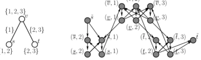
For both problems MFMI and MCFMI, we denote by G = (V, E) the graph induced by the sharing function X, also
Fig. 1. The graph G and its transformation in the direct graph G′. W(s) = {1, 2}, W (v) = 1, 2, 3, W (t) = X(v, t) = {2, 3}, and X(s, v) = {1}. v s t {2, 3} {1, 2} {1, 2, 3} {1} {2, 3} ˜t (s, 1) (t, 3) (t, 3) (s, 1) (t, 2) (t, 2) (v, 3) (v, 3) (v, 2) (v, 2) (s, 2) (s, 2) ˜ s (v, 1) (v, 1)
referred as the input graph. GraphG can be easily computed
from X in time O(|V | + |E|). Note that we can consider
two variants of theMCFMI problem: the parameter k can be
considered as part of the input (this is called the unbounded
case), or k may be a fixed constant (the bounded case). In
both cases we assumek ≥ 2, since the case k = 1 admits an
obvious solution given by a shortest path connectings to t of
maximum bandwidthb(1). The case where the cost function
is constant for each interface is called the unit cost case. III. PRELIMINARY RESULTS
The algorithms given in this paper for the general cases of
MFMI and MCFMI are both based on a transformation of
the graphG = (V, E) into a directed graph G′ = (V′, A). G′
is defined so that bandwidths and costs are associated to arcs rather than to interfaces. Informally, for each interface of each node, there is an arc which has the same cost and bandwidth of the considered interface. The head of each of such arcs is connected to the tail of another arc of the same kind if they share an interface or they represent different interfaces of the same node. As each of these arcs is associated with the cost and the bandwidth of the interface it represents, the activation of an interface is modeled with the usage of one of these arcs, preserving the bandwidth constraints and the activation costs. Moreover, although the arcs are directed, the possibility to communicate towards and from every node of the original graph is preserved (see also Fig. 1).
Formally, for each nodev ∈ V and each interface i ∈ W (v),
there are two nodes inV′ denoted as(v, i) and (v, i): V′= {(v, i), (v, i) | v ∈ V, i ∈ W (v)} ∪ {˜s, ˜t}.
The arcs are the following:
A = {((v, i), (v, i)) | v ∈ V, i ∈ W (v)} ∪ {((v, i), (v, j)) | v ∈ V, i, j ∈ W (v) s.t. i 6= j} ∪
{((u, i), (v, i))| i ∈ X(u, v)} ∪ ©(˜s, (s, i)), ((t, j), ˜t) | i ∈ W (s), j ∈ W (t)ª .
The capacity of each arc ((v, i), (v, i)) is set to b′((v, i), (v, i)) = b(i) whereas the capacity of each other arc
inA is unlimited and it is 0 for each pair in V × V \ A. The
cost c′(a) of each arc a = ((v, i), (v, i)) is set to c(i) and it
is0 for the remaining arcs.
Given a flow function f′ from s to ˜˜ t for G′, we define a
flow functionf from s to t in G as follows: f (u, v, i)=½f
′((u, i), (v, i)) − f′((v, i), (u, i)) if i ∈ X(u, v)
The allocation of active interfaces at nodeu for MCFMI is
defined as WA(u) = {i ∈ W (u) | ∃v ∈ V s.t. f (u, v, i) 6= 0}. In order to address concurrently MCFMI and MFMI, we
defineWAforMFMI as equivalent to the assignment function W induced by the sharing function X. Note that both functions f and WAcan be computed in polynomial time once function f′ is known.
The next lemma shows that, if we apply the above transfor-mation to an instanceI of MFMI or MCFMI and we compute
a flow function f and an assignment of interfaces WA for I
by using the above definition on some flow functionf′ ofG′,
thenf satisfies Properties 1–4 needed by both the definitions
of MFMI and MCFMI.
Lemma 3.1: Let f and WA be a flow function and an
assignment of interfaces defined as above, then 1) f (u, v, i) = −f (v, u, i) ∀ u, v ∈ V and i ∈ I;
2) f (u, v, i) = 0 if WA(u) ∩ WA(v) ∩ X(u, v) = ∅ ∀ u, v ∈ V and i ∈ I;
3) P
v∈V :f (u,v,i)>0f (u, v, i) ≤ b(i) ∀ u ∈ V and i ∈ I; P
v∈V :f (v,u,i)>0f (v, u, i) ≤ b(i) ∀ u ∈ V and i ∈ I;
4) P
v∈V,i∈If (u, v, i) = 0 ∀ u ∈ V \ {s, t}.
Proof: We recall that, by definition of a flow function for
a directed flow network:
0 ≤ f′(x, y) ≤ b′(x, y), for each(x, y) ∈ A (a)
f′(x, y) = −f′(y, x), for eachx, y ∈ V′ (b)
X x∈V′
f′(x, y) = 0, for eachy ∈ V′\ {˜s, ˜t}. (c)
In the following we prove the four properties.
1) If i 6∈ X(u, v), then f (u, v, i) = f (v, u, i) = 0. In fact,
by definition of f and by Property (b)
f (u, v, i) = f′((u, i), (v, i)) − f′((v, i), (u, i)) = − (f′((v, i), (u, i)) − f′((u, i), (v, i))) = −f (v, u, i).
2) If WA(u) ∩ WA(v) ∩ X(u, v) = ∅, then for each i ∈ I
eitheri 6∈ WA(u) or i 6∈ WA(v) or i 6∈ X(u, v). If i 6∈ WA(u),
then by definition ofWA(u) f (u, v, i) = 0. If i 6∈ WA(v), then
by definition ofWA(v), f (v, u, i) = 0, moreover by the above
property, f (u, v, i) = −f (v, u, i) = 0. If i 6∈ X(u, v), then by
definition of f , f (u, v, i) = 0.
3) We formally provide only the proof for the first inequality as the second one follows from similar argu-ments. By definition of f , P
v∈V :f (u,v,i)>0f (u, v, i) = P
v∈V :f (u,v,i)>0(f′((u, i), (v, i)) − f′((v, i), (u, i))) .
By Property (a), for each v ∈ V , f′((v, i), (u, i)) ≥ 0 and f′((u, i), (v, i)) ≥ 0, then
P
v∈V :f (u,v,i)>0(f′((u, i), (v, i)) − f′((v, i), (u, i))) ≤ P
v∈V :f (u,v,i)>0f′((u, i), (v, i)).
By the definition of b′ and Property (a), X
v∈V :f (u,v,i)>0
f′((u, i), (v, i)) ≤ X v∈V
f′((u, i), (v, i)).
By Property (c), applied to (u, i), P
v∈V f′((u, i), (v, i)) = f′((u, i), (u, i)) −P
j∈I\{i}f′((u, i), (u, j)). Again by
Prop-erty (a), f′((u, i), (u, j)) ≥ 0, for each j ∈ I \ {i}, then f′((u, i), (u, i)) − P
j∈I\{i}f′((u, i), (u, j) ≤
f′((u, i), (u, i)) ≤ b(i). The last inequality directly follows
from Property (a).
4) By definition off , f (u, v, i) = 0 if v = u or i 6∈ X(u, v),
hence P
v∈V,i∈If (u, v, i) = P
v∈V \{u} i∈X(u,v)
(f′((u, i), (v, i)) −f′((v, i), (u, i))).
By Property (c), applied to nodes (u, i), P
v∈V \{u} i∈X(u,v)
f′((u, i), (v, i)) = P
v∈V \{u} i∈X(u,v)
µ
f′((u, i), (u, i)) −P j∈X(u,v)
j6=i
f′((u, i), (u, j)) ¶
.
Again, by Property (c), applied to nodes (u, i), P
v∈V \{u} i∈X(u,v)
f′((v, i), (u, i)) = P
v∈V \{u} i∈X(u,v)
µ
f′((u, i), (u, i)) −P j∈X(u,v)
j6=i
f′((u, j), (u, i)) ¶
.
Hence, P v∈V \{u} i∈X(u,v)
(f′((u, i), (v, i)) − f′((v, i), (u, i))) = P v∈V \{u} i∈X(u,v) µ P j∈X(u,v) j6=i
f′((u, j), (u, i))− P
j∈X(u,v) j6=i
f′((u, i), (u, j)) ¶
= 0,
in fact, for any pair of interfacesp and q such that p 6= q, we
have that, wheni = p and j = q, the related term of the above
sum is f′((u, q), (u, p)) − f′((u, p), (u, q)), on the contrary,
wheni = q and j = p, it is f′((u, p), (u, q))−f′((u, q), (u, p))
and hence the overall sum is 0.
IV. COMPUTATIONAL COMPLEXITY
In this section we study the computational complexity of
MFMI and MCFMI. We first prove that MFMI is optimally
solvable in polynomial time in the general case, we then focus onMCFMI. We prove that MCFMI is NP -hard even in the
restricted case of unit cost, fixed k ≥ 2, and fixed ∆ ≥ 3.
Then we consider graphs of bounded degree ∆ ≤ 2. As
announced in Table I, we prove that, when the number of interfaces k is fixed, the problem can be optimally solved in
polynomial time. On the other hand, if k is unbounded, we
show that the problem remainsNP -hard. Moreover, when the
bandwidth function b is a constant, then MCFMI is solvable
in polynomial time (see Corollary 5.3 in the next section).
A. General Case
LetA be an algorithm that finds a maximum flow in a graph H = (VH, EH) in polynomial time PA(|VH| + |EH|).
Theorem 4.1: MFMI is optimally solvable within
O(|V |k2+ |E| + P
A(|V |k2+ |E|)) time.
Proof: Given an instanceI1ofMFMI, the algorithm first
transforms the graphG and the function b of I1 into a graph G′ and a function b′ as described in Section III, obtaining an
instanceI2 of the classical maximum flow problem. Then, in
polynomial time, it finds a maximal flow function f′ for I 2
by using a maximum flow algorithm. Finally, the algorithm obtains a maximal flow function f for I1 from f′ by using
the transformation given in Section III. The computational time required by such an algorithm is given by the cost of transforming I1 into I2 and that of solvingI2. As the graph
Fig. 2. The subgraphs used in the proofs of Theorems 4.2 and 5.1. r w1 y1 x1 w2 y2 x2 N(ℓ) xℓ−1 yℓ−1 wℓ−1 xℓ yℓ wℓ T(5)
the first cost is O(|V |k2 + |E|) while the second one is O(PA(|V |k2+ |E|)).
We now show that f is an optimal solution for I1.
By Lemma 3.1, f satisfies properties 1–4 of the
defini-tion of MFMI. We show that f is maximal by
contradic-tion. We recall that by definition of maximal flow function,
P
v∈V′f′(˜s, v) is maximal. By contradiction, let us suppose that there exists a flow functionf′′ : V × V × I → Z+
0 for I1 such that Pv∈V,i∈If′′(s, v, i) >
P
v∈V,i∈If (s, v, i). We
define a flow functionf′′′: V′× V′→ Z+
0 for I2 as follows,
ifi ∈ X(u, v),
f′′′((u, i), (v, i)) = ½
f (u, v, i) if f (u, v, i) > 0 0 otherwise.
For edges in {((v, i), (v, i)) | v ∈ V, i ∈ W (v)} ∪ {((v, i), (v, j)) | v ∈ V, i, j ∈ W (v) s.t. i 6= j}, f′′′ is
defined in order to satisfy the flow conservation constraints, and it is0 for any other pair in V × V .
Similar arguments as Lemma 3.1 can be used to show that
f′′′ fulfills the properties of flow functions and that X v∈V′ f′′′(˜s, v) = X v∈V,i∈I f′′(s, v, i), X v∈V′ f′(˜s, v) = X v∈V,i∈I f (s, v, i). It follows that P v∈V′f ′′′(˜s, v) = P v∈V,i∈If′′(s, v, i) > P v∈V,i∈If (s, v, i) = P v∈V′f ′(˜s, v), a contradiction to the maximality off′.
Theorem 4.2: MCFMI is strongly NP -hard even when
restricted to the unit cost interface case for any fixed∆ ≥ 3
andk ≥ 2.
Proof: We prove that the underlying decisional problem,
denoted byMCFMID, is in generalNP -complete. We need to
add one further boundD ∈ Z+0 such that the problem consists
in deciding whether there exists an activation function which induces a total cost of the active interfaces of at mostD.
Given an allocation function of active interfaces for an instance ofMCFMID, checking whether the induced subgraph
allows a bandwidth greater than or equal to B of total cost
smaller than or equal toD requires linear time in the number
of edges of the input graph G. Then, MCFMID is in NP .
The proof proceeds by a polynomial reduction from the well-known Exact Cover by3-Sets problem. The problem is known
to beNP -complete [15] and it can be stated as follows:
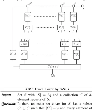
Fig. 3. The graph G in the transformation from X3C to MCFMID.
T(3) T(3) T(3) s N(3) N(3) N(3) c1 c2 c|C| N(1) N(1) N(1) N(1) T(3q + 1) t T(µ) T(µ) T(µ)
X3C: Exact Cover by 3-Sets
Input: Set S with |S| = 3q and a collection C of
3-element subsets ofS.
Question: Is there an exact set cover for S, i.e. a subset C′ ⊆ C such that |C′| = q and every element of S belongs to exactly one member of C′?
Given an instance of X3C, we construct an instance of MCFMID where the graph G consists of copies of
sub-graphs N (ℓ) and T (ℓ), ℓ ≥ 1 (see Fig. 2). Subgraph N (ℓ)
consists of 3ℓ nodes {x1, x2, . . . , xℓ} ∪ {y1, y2, . . . , yℓ} ∪ {w1, w2, . . . , wℓ} and edges {xi, xi+1}, {wi, wi+1}, for i = 1, 2, . . . , ℓ − 1 and {xi, yi}, {yi, wi}, for i = 1, 2, . . . , ℓ.
SubgraphT (ℓ) is a binary tree consisting of a complete binary
treeBT with 2⌈log2ℓ⌉− 1 nodes, and ℓ nodes adjacent to the leaves of BT . These nodes are the only leaves of T (ℓ), i.e.
every leaf ofBT is connected to at least one leaf of T (ℓ). We
callr the root of T (ℓ). Note that, each path from r to a leaf
ofT (ℓ) is constituted of ⌈log2ℓ⌉ + 1 nodes. Moreover, when ℓ = 1, BT is empty and T (ℓ) consists of a single node.
For the sake of simplicity, in this proof we first define the graphG and then we define functions W and X accordingly.
See Fig. 3 for a visualization ofG. Let s and t be two nodes of G. For each element Ci ofC, i = 1, 2, . . . , |C|, G contains a
nodeci, a copy ofN (3), denoted as Ni(3) and a copy of T (3),
denoted asTi(3), with root ri and leavesli
1,li2,li3. Nodesxi1
andwi
3 of Ni(3) are adjacent to ci and ri, respectively. All
nodesci form a pathP in G, that is {ci, ci+1} is an edge of G, for i = 1, 2, . . . , |C| − 1. Node s of G is adjacent to c1,
while node c|C| is adjacent to node x0
1 belonging to a copy N0(1) of N (1) with nodes x0
1,y10andw01.
Letej,j = 1, 2, . . . , 3q, be the elements of S and let µ(ej)
be the number of setsCi∈ C containing ej, for eachj. Let µ = maxj{µ(ej)}. For each element ej,G contains a copy of T (µ), called Tj(µ), with root rj, and a copyNj(1) of N (1),
with nodesxj1,yj1andwj1. Rootrj is adjacent toxj
1∈ Nj(1),
for each j = 1, 2, . . . , 3q. If ej is in Ci, for some i and j,
These edges are pairwise disjoint. Note that, even if each leaf of Ti(3), i = 1, 2, . . . , |C| is adjacent to a leaf in Tj(µ), for
somej ∈ {1, 2, . . . , 3q}, the contrary is not true: there could
be a leaf of Tj(µ), for some j, not adjacent to any leaf of Ti(3), i = 1, 2, . . . , |C|.
G also contains a copy of T (3q+1), having the root adjacent
to node t, and leaves adjacent to nodes wj1,j = 0, 1, . . . , 3q.
The set of interfaces I is {1, 2}, with c(1) = c(2) = 1 and b(1) = 1, b(2) = 3q + 1.
FunctionW is defined as follows. All the nodes in G have
interface 2 apart from nodes labeled y in the copies of N (1)
andN (3). All the nodes in the copies of N (1) and N (3) have
interface 1: no further node in G has interface 1. Function X
is defined as follows, given two nodesu, v in G, X(u, v) =
½
W (u) ∩ W (v) if{u, v} ∈ E
∅ otherwise.
When all the interfaces of the nodes in copies of N (ℓ)
(T (ℓ), resp.), for a certain ℓ ≥ 0, are active the total cost
is 5ℓ (2⌈log2ℓ⌉ − 1 + ℓ, resp.). In T (ℓ), when only the interfaces of the nodes in a single path from r to a leaf are
active, the total cost is ⌈log2ℓ⌉ + 1. Let B = 3q + 1 and D = |C| + q(42 + 3⌈log2µ⌉) + 2⌈log2(3q+1)⌉+ 7.
Assume thatX3C has a positive answer, i.e., there exists an
exact set coverC′ = {C
i1, Ci2, . . . , Ciq} ⊆ C for S. We show that also MCFMID has a positive answer, i.e., there exists an
activation functionWAof the available interfaces such that the
bandwidth allowed from s to t is bigger than or equal to B
and the total cost is smaller than or equal toD. Function WA
is defined as follows. Along with interfaces of nodes s, t, all
the interfaces of nodes in T (3q + 1), Nj(1), j = 0, 1, . . . , 3q,
andci,i = 1, 2, . . . , |C|, are active. All the interfaces of nodes
inNij(3) and Tij(3), for each C ij ∈ C
′,j = 1, 2, . . . , q, are
active. Moreover, if ei ∈ S is covered by Cj ∈ C′, then all
the interfaces of nodes in Tj(µ) belonging to the path from rj to a leaf inTi(3) are active. No further interface is active.
The flow function is defined as 1 in nodes y of active copies
of N (1) and N (3) and in the remainder of G it is defined to
satisfy the flow conservation constraints.
The total cost of active interfaces is given by 2, for nodes s and t; |C|, for nodes ci ∈ P , i = 1, 2, . . . , |C|; 15q + 6q for
nodes inNij(3) and Tij(3), j = 1, 2, . . . , q; 3q(⌈log
2µ⌉ + 1)
for nodes in Tj(µ), j = 1, 2, . . . 3q; 5(3q + 1) for nodes in Nj(1), j = 0, 1, . . . 3q; and 2⌈log2(3q+1)⌉+ 3q for nodes in
T (3q + 1). Summing up all the values we obtain a cost equal
toD.
Regarding the total bandwidth, note that a copy ofN (ℓ) has
a maximum bandwidth of ℓ. As X3C has a positive answer,
each element of S is covered, then the flow through each
subgraph Nj(1), j = 1, 2, . . . , 3q, is exactly 3q. As all the
interfaces in P are active, we also have a flow of 3q + 1
throughN0(1) that reaches t through the T (3q + 1) subgraph.
ThenMCFMID has a positive answer.
Now, let us assume we have a positive answer toMCFMID.
As the total flow received by t is greater than or equal to B = 3q +1, there is a flow of value 1 in each subgraph Nj(1), j = 0, 1, . . . , 3q, meaning that each element of S is covered.
Let us suppose, by contradiction, that the flow reaching the
Nj(1), j = 1, 2, . . . , 3q subgraphs, implies the activation of
the interfaces in q′ > q subgraphs among the Ni(3), i = 1, 2, . . . , |C| copies of N (3). In this case there will be q′
1
subgraphs having one unit of flow,q′
2subgraphs having2 units
of flow, and q′
3 subgraphs having 3 units of flow such that q′
1+ 2q′2+ 3q′3= 3q.
The total cost for the interfaces activation is:2, for nodes s
andt; |C|, for nodes in P (all the interfaces in P are active as N0(1) receives one unit of flow); 7q′
1+11q2′+15q3′ for nodes in Ni(3); 6q for nodes in Ti(3), i = 1, 2, . . . , q; 3q(⌈log
2µ⌉+1)
for nodes in Tj(µ), j = 1, 2, . . . 3q; 5(3q + 1) for nodes in Nj(1), j = 0, 1, . . . 3q, and 2⌈log2(3q+1)⌉+ 3q for nodes in
T (3q + 1).
Then the total cost is |C| + q(27q + 3⌈log2µ⌉) + 2⌈log2(3q+1)⌉+ 7 + 7q′
1+ 11q′2+ 15q′3. As7q′1+ 11q2′+ 15q3′ > 5(q′
1+ 2q2′ + 3q′3) = 15q, the total cost is greater than D,
a contradiction. Hence there are exactlyq subgraphs Nij(3),
j = 1, 2, . . . , q with 3 units of flow each and the corresponding
sets Cij,j = 1, 2, . . . , q, represent a solution for X3C.
B. Particular cases forMCFMI, ∆ ≤ 2
Theorem 4.2 shows thatMCFMI is NP -hard even for fixed ∆ ≥ 3 and k ≥ 2. As the case where k = 1 is trivial, we now
focus on the case that∆ ≤ 2. For ∆ ≤ 1, the input graph can
be composed of either one single node or two nodes connected by one edge. In the first case, there are no interfaces to be activated, as the source and the destination coincide. In the second case, the problem already starts to be interesting.
Theorem 4.3: MCFMI is polynomially solvable within O(1) time in the bounded case with ∆ = 1.
Proof: MCFMI can be solved by an exhaustive search
among all the possible combinations of interfaces shared by
s and t. The number of such combinations is O(2k). Among
them, a resolution algorithm has to choose the cheapest one that guarantees at leastB bandwidth.
For the unbounded case, i.e., whenk is not a given constant,
the same arguments of Theorem 4.3 do not apply toMCFMI
as the provided algorithm would show an exponential behavior. Surprisingly, in this setting the problem turns out to be already
NP -hard by means of a simple polynomial transformation
from the well known Minimization Knapsack problem [16], [17].
M inKP : Minimization Knapsack
In.: An integer d ∈ Z+0 and a set of n items, each
one having weight wi ∈ Z+0 and profit pi ∈ Z+0, i = 1, 2, . . . , n.
Sol.: An allocation of variables yi ∈ {0, 1}, for i = 1, 2, . . . , n, such thatPn
i=1wiyi≥ d
Aim: Minimize Pn i=1piyi.
M inKP problem is the corresponding minimization version
of the Knapsack problem. In other words, the goal is to minimize the profits of the items that remain out of the knapsack. If xi, i = 1, 2, . . . , n, are the variables selecting
the items for the classical knapsack problem and c ∈ Z+0
its capacity, then the problem can be solved by means of
M inKP , by setting d = Pn
i=1wi − c and yi = 1 − xi, i = 1, 2, . . . , n.
When ∆ = 1, that is when the input graph G consists of
a single edge from s to t, the required solution must select
a subset of interfaces among the ones shared by s and t in
such a way that a bandwidth of B is guaranteed, and the
cost for activating such interfaces is minimized. Intuitively, this particular case of MCFMI is equivalent to the M inKP
problem.
Theorem 4.4: MCFMI is polynomially equivalent to
M inKP in the unbounded case with ∆ = 1.
Proof: We have to show that there exist two polynomial
time algorithms A and B such that, for each instance I1 of M inKP , A(I1) returns an instance I2 of MCFMI, for any
solution σ′ of I
2, B(σ′) = σ is a solution for I1, and the
values of solutions σ and σ′ are equal. Moreover, we have
to show that there exist two polynomial time algorithmsA−1
andB−1such that, for each instanceI
2ofMCFMI, A−1(I2)
returns an instance I1 of M inKP , for any solution σ of I1, B−1(σ) = σ′ is a solution forI
2, and the values of solutions σ and σ′ are equal.
We now show the first part of the above statement by defin-ing the polynomial algorithms A and B. Given an instance I1 ofM inKP , we consider an instance I2of MCFMI made
of nodes s and t, and, for each item i of I1, an interface i
shared between s and t with cost c(i) = 12pi and bandwidth b(i) = wi. Hence W (s) = W (t), moreover, function X is
defined as X(s, t) = W (s). Finally, let k = n and B = d.
Note that, if, for somei, piis an odd number, we can multiply
all the profits pi of a factor 2 in order to havec(i) ∈ Z+0 for
eachi = 1, 2, . . . , n. This does not affect the generality of the
proof as it is enough to divide by 2 the value of the objective function for the solution of I1 which will be defined in the
following. A feasible solution forI2selects a set of interfaces W , by means of an activation function, in such a way that
B ≤ P i∈Wb(i). As d = B ≤ P i∈Wb(i) = P i∈Wwi
and the cost of activating interfaces in W at both s and t
is2P
i∈Wc(i) = P
i∈Wpi, we can define algorithmB as the
algorithm which selects itemsW in order to output a solution
forI1. Finally, bothA and B are polynomial time algorithms.
This proves the first part of the theorem. For the second part of the theorem, it is enough to note that algorithms A and B
can be naturally inverted.
Corollary 4.5: MCFMI is NP -hard in the unbounded case
with∆ = 1 and it admits a pseudo-polynomial-time algorithm.
For∆ = 2, the input graph of MCFMI is either a path or
a cycle. Clearly, from Corollary 4.5, MCFMI remains NP
-hard in the unbounded case. The following theorem gives a polynomial time algorithm for the bounded case. In the next section, we will derive a pseudo-polynomial-time algorithm for the unbounded case.
In the remainder, for a set of interfaces W , we denote as c(W ) the cost of activating the interfaces in W , formally: c(W ) =P
i∈Wc(i).
Theorem 4.6: MCFMI is solvable within O(|V |) time in
the bounded case when the input graph is a path.
Proof: Let us denote the input path as a sequence
of n nodes: s ≡ x0, x1, . . . , xn−1 ≡ t. Given a node xℓ, 1 ≤ ℓ ≤ n − 1, γ(xℓ) denotes the set of sub-sets
of interfaces of xℓ, shared with xℓ−1, whose total
band-width is greater than or equal to B, formally: γ(xℓ) = ©W ⊆ X(xℓ, xℓ−1)
¯
¯ Pi∈Wb(i) ≥ Bª. Then, the minimum
cost is given by:
OPT= min {2c(W1) + c(W2\ W1) + c(W2) + . . . . . . + c(Wn−1\ Wn−2) + c(Wn−1) | W1∈ γ(x1), W2∈ γ(x2), . . . , Wn−1∈ γ(xn−1)} ,
where 2c(W1) is the cost of interfaces used to connect x0
to x1 and c(Wℓ\ Wℓ−1) + c(Wℓ) is the cost of interfaces
used to connect xℓ−1 to xℓ, 2 ≤ ℓ ≤ n − 1. In particular, c(Wℓ\Wℓ−1) is the cost of activating in xℓ−1the interfaces in Wℓnot contained inWℓ−1 andc(Wℓ) is the cost of activating
interfacesWℓ inxℓ.
For each 1 ≤ ℓ ≤ n − 1, let us define the function Cℓ : γ(xℓ) → Z+0 as the minimum cost needed to establish
a communication path from s to node xℓ with bandwidth
guarantee greater than or equal to B by activating interfaces W ∈ γ(xℓ) in xℓ, formally:
Cℓ(W ) = min {2c(W1) + c(W2\ W1) + c(W2) + . . . . . . + c(W \ Wℓ−1) + c(W ) |
W1∈ γ(x1), W2∈ γ(x2), . . . , Wℓ−1∈ γ(xℓ−1)} .
By definition, OPT = minW∈γ(xn−1)Cn−1(W ). Hence it is enough to show that functions Cℓ, for each 1 ≤ ℓ ≤ n − 1,
can be computed in O(n) time. By cut-and-paste arguments,
it follows that:
Cℓ(W ) = min Wℓ−1∈γ(xℓ−1)
{Cℓ−1(Wℓ−1) +c(W \ Wℓ−1) + c(W )} .
Therefore, functions Cℓ, can be computed by using dynamic
programming starting from C1(W ) = 2c(W ), for each W ∈ γ(x1). Moreover, as k is a bounded constant, |γ(xℓ)| ≤ 2k = O(1). Hence, given 1 ≤ ℓ ≤ n − 1 and W ∈ γ(x
ℓ),
computingCℓ(W ) requires O(1) time and computing function Cℓ requires O(1) time. Then, all the functions Cℓ, for all 1 ≤ ℓ ≤ n − 1, can be computed in O(n) time.
When the input graph is a cycle, since there are two paths froms to t, it is not always clear how the bandwidth B must
be split among the two possible ways. However, the following theorem can be stated for the bounded case.
Theorem 4.7: MCFMI is solvable within O(|V |) time in
the bounded case when the input graph is a cycle.
Proof: LetP1andP2be the two edge-disjoint paths from s to t composing the input cycle. As by definition, b(i) ∈ Z+0, 1 ≤ i ≤ k, the required flow B is provided by summing two
integersβ1 andβ2 that are the contributions to the total flow
passing viaP1andP2, respectively. The valuesβ1andβ2vary
among all the integers obtainable by summing the bandwidths provided by each possible subset of interfaces, i.e.,β1andβ2
can assume at most2k values. For each subset of interfaces of s and for each subset of interfaces of t, the algorithm proposed
by Theorem 4.6 is applied to solve the MCFMI instance
arising forP1 with boundβ1, and the one arising forP2with
them requires 2k tests, one for each possible value ofβ 1. As k = O(1), then 23k = O(1). Among the obtained solutions,
we choose the cheapest one which guarantees a flow of at least
B from s to t. Such algorithm requires to run O(1) times the
algorithm in Theorem 4.6 and hence it requiresO(|V |) overall
computational time.
V. APPROXIMATION
In this section, we study the approximation properties of
MCFMI. We first show that, unless P = NP , MCFMI cannot
be approximated within a factor of Ω(log B), or within a
factor of Ω(log log |V |), even for fixed ∆ ≥ 3 and fixed k ≥ 3. We also provide a bmax
M -approximation algorithm for
the general case, where bmax = maxi∈Ib(i) and M is the
greatest common divisor among the bandwidths allowed by the interfaces and the required bandwidthB. Finally, we analyze
the case of fixed∆ ≤ 2. As in the previous section, it has been
shown that, in this case, MCFMI is polynomially solvable
if k is fixed, then we focus on the approximability of the
unbounded case. We give two results which show that, if
∆ = 1 or the input graph is a path, then MCFMI admits
a FPTAS, while in the case that the input graph is a cycle the approximability of MCFMI remains open.
A. General case
Theorem 5.1: MCFMI cannot be approximated within a
factor of Ω(log B), or within a factor of Ω(log log |V |), for
any fixed ∆ ≥ 3 and k ≥ 3, unless P = NP .
Proof: We will show the statement by providing an approximation gap preserving reduction [18] from the Set Cover (SC) problem to MCFMI.
SC: Set Cover
In: A set U with n elements and a collection S = {S1, S2, . . . , Sq} of subsets of U .
Sol: A cover for U , i.e. a subset S′ ⊆ S such that every
element ofU belongs to at least one member of S′.
Aim: Minimize|S′|.
We first show that there exists a polynomial time algorithm that transforms any instance I1 of SC into an instance I2 of MCFMI such that the optimum value SOL∗
SC onI1 for the
problem SC is greater than or equal to the optimum value SOL∗
MCFMI onI2 for the problemMCFMI.
The transformation is similar to the one provided for Theo-rem 4.2 (see Fig. 4). The graphG is given by two nodes s and t where s is adjacent to the root node of a copy of T (|S|) and t to the root node of a copy of T (n). For each element Si of S, i = 1, 2, . . . , |S|, G contains a copy of N (1), denoted by Ni(1) and a subgraph T (|Si|) with root ri adjacent to node wi 1∈ N i (1). Each node xi 1∈ N i (1) is adjacent to a different
leaf of T (|S|). Let uj, j = 1, 2, . . . , |U |, be the elements of U and let µj be the number of setsSi∈ S containing uj, for
each j. For each element uj,G contains a subgraph T (µj),
with root rj, and a copy Nj(1) of N (1), with nodes xj 1, y
j 1
and wj1. Root rj is adjacent to xj1 ∈ Nj(1), and each node xj1 ∈ Nj(1) is adjacent to a different leaf of T (n), for each j = 1, 2, . . . , n. If uj ∈ Si, for somei and j, then there is an
Fig. 4. The graph G in the transformation from X3C to MCFMID.
N(1) N(1) N(1) t T(n) T(µn) T(µ2) T(µ1) s T(|S|) N(1) N(1) N(1) T(|S2|) T(|Sq|) T(|S1|)
edge from a leaf of T (|Si|) to a leaf of T (µj). These edges
are pairwise disjoint.
The set of interfaces is {1, 2, 3}, with c(1) = 0, c(2) = 1, c(3) = 0 and b(1) = n, b(2) = n, b(3) = 1. All the nodes inG have interface 1 apart from the central nodes of the n + |S| copies of the N (1) graph. All the nodes in Ni(1) have interface2, for each i = 1, 2, . . . , |S|. All the nodes in Nj(1)
have interface 3, for each j = 1, 2, . . . , n. Then, X(u, v) =
½
W (u) ∩ W (v) if{u, v} ∈ E
∅ otherwise.
Let B = n, we denote by SOLSC(I1, σ1) the value of
the cost function of SC for a solution σ1 on instance I1,
and let SOL∗
SC(I1) be the optimal cost for SC on instance I1. Moreover, let us denote by SOLMCFMI(I2, σ2) the cost
function ofMCFMI of a solution σ2 on instance I2, and let
SOL∗
MCFMI(I2) be the optimal cost for MCFMI on instance I2.
Let us assume that we have an optimal solution
{Si1, Si2, . . . , Sim} for SC. Then, by activating all the
in-terfaces 1 and 3 in G and the interfaces 2 only in the nodes of subgraphs Nij
(1), j = 1, 2, . . . , |S|, we obtain a feasible solution σ for I2 such that SOL(I2, σ) ≤ 3SOL∗SC(I1),
hence:SOL∗
MCFMI(I2) ≤ 3SOL∗SC(I1).
Now we show that it is possible to transform in polyno-mial time any solution σ2 for the instance I2 of MCFMI
into a solution σ1 for the instance I1 of SC such that 3SOLSC(I1, σ1) = SOLMCFMI(I2, σ2). A solution σ2
con-sists of a flow of n units passing through each subgraph Nj(1), j = 1, 2, . . . , n, corresponding to a covering of all
the elements in U . A solution σ1 then consists of the sets Si1, Si2, . . . , Sim corresponding to those subgraphs N
ij
(1), j = 1, 2, . . . , m, having a positive flow. As consequence, 3SOLSC(I1, σ1) = SOLMCFMI(I2, σ2).
If there exists an α factor approximation algorithm A
approxima-tion algorithm for SC. In fact, given an instance I1 of SC, we could find a solution σ1 for SC by using the
above transformation from I1 to an instance I2 of MCFMI
and applying A to find an α-approximate solution σ2.
Hence obtaining SOLSC(I1, σ1) = 13SOLMCFMI(I2, σ2) ≤ α
3SOL ∗
MCFMI(I2) ≤ αSOL∗SC(I1). In [19], the authors show
that no approximation algorithm forSC exists with an
approx-imation factor less than Ω(log n). Then there is no algorithm
forMCFMI with an approximation factor less than Ω(log B),
since we set B = n. By observing that for the instance I2, |V | ≤ a1|S| + a2n + a3 ≤ 2na1+ a2n + a3 ≤ 2na4 for
certain constants a1, a2, a3 and a4 = 3 max{a1, a2, a3}, we
have n ≥ log(|V |/a4). By using the same inapproximability
result as before, we obtain the thesis.
Theorem 5.1 also holds when the number of interfaces is unbounded. We now provide a bmax
M -approximation algorithm
for any instance of MCFMI, where bmax is the maximum
bandwidth value among the interfaces in I and M is the
greatest common divisor among the bandwidths allowed by the interfaces and the required bandwidth B. The algorithm
consists in relaxingMCFMI to the well-known Integral Mini-mum Cost Flow (IMCF ) problem [20]. In the proof of the next
theorem, we transform an instance ofMCFMI into an instance
of IMCF , and we show that such a transformation guarantees
an approximation factor of bmax
M . Let A be an algorithm
which optimally solves IMCF on a graph H = (V′, E′) in
polynomial time PA(|V′| + |E′|).
Theorem 5.2: There exists a polynomial time bmax M
-approximation algorithm for MCFMI which requires
O(|V |k2+ |E| + P
A(|V |k2+ |E|)) time.
Proof: Given an instance I1 of MCFMI, the algorithm
works in four phases. First it transforms the graph G and
functions b and c of I1 into a graph G′ and functions b′
and c′ as described in Section III. Hence, we obtain an
instance I2 of an equivalent problem defined on a directed
graph G′ = (V′, A) without using multiple interfaces but
associating costs and bandwidths only to arcs in A. The aim
of such problem is finding a flow function which satisfies flow constraints and such that the flow going from the sources to˜
the sink ˜t is greater than or equal to B. Then, the algorithm
transforms I2 into an instance I3 of IMCF . In the third
phase, the algorithm solves I3 by using a known algorithm
and, finally, it transforms the obtained solution for I3 into a
solution forI2made of a flow functionf′. Functionf′ can be
transformed into a solution forI1, as described in Section III,
obtaining a flow function f and an assignment of interfaces WA.
In the following, we first show that the problems of solving
I1 andI2 are equivalent, then we show how to approximate
an optimal solution for I2 by optimally solvingI3.
Given a solution for I2, which defines a flow functionf2,
we can define a solution for I1 by assigning a flow function f1 as explained in Section III, that is,
f1(u, v, i)=½f0,2((u, i), (v, i)) − f2((v, i), (u, i)) if i ∈ X(u, v)otherwise.
Vice versa, given a solution for I1, which defines a flow
function f′
1, we can define a solution for I2 by assigning a
flow functionf′
2 as follows, ifi ∈ X(u, v), f2′((u, i), (v, i)) =
½
f1′(u, v, i) iff1′(u, v, i) > 0 0 otherwise.
In edges in {((v, i), (v, i)) | v ∈ V, i ∈ W (v)} ∪ {((v, i), (v, j)) | v ∈ V, i, j ∈ W (v) s.t. i 6= j}, f′
2 is defined
in order to satisfy flow conservation constraints, and it is 0
for any other pair inV × V . We now prove that the feasibility
of f2 (f1′, resp.) implies the feasibility of f1 (f2′, resp.). By
Lemma 3.1, properties 1–4 of the definition of MCFMI
follows. Moreover, similar arguments can be used to show that f′
2 satisfies flow constraints and that X v∈V′ f2(˜s, v) = X v∈V,i∈I f1(s, v, i) X v∈V,i∈I f1′(s, v, i) = X v∈V′ f2′(˜s, v).
Hence, to show property 5 of the definition of MCFMI,
it is enough to note that if P
v∈V′f2(˜s, v) ≥ B (P
v∈V,i∈If1′(s, v, i) ≥ B, resp.) then P
v∈V,i∈If1(s, v, i) ≥ B (P
v∈V′f ′
2(˜s, v) ≥ B, resp.). This shows that the feasibility
of f2 (f1′, resp.) implies the feasibility of f1 (f2′, resp.). To
conclude the first part of the proof, note that, the cost of f2
(f′
1, resp.) is equal to the cost off1 (f2′, resp.) as the cost of
arcs ((v, i), (v, i)) in A is c(i) and it is 0 for any other arc.
By the above discussion it follows that we can solve I1 by
solvingI2.
We find an approximate solution forI2by using an IMCF
instance. The IMCF problem consists of finding an integral
flow greater than or equal to a given quantityΘ between two
nodes in a directed graphH where each arc a has a capacity β(a) and cost χ(a). The objective is to minimize the function P
a∈A+χ(a) · f′′(a), where f′′(a) is the flow on arc a and
A+ is the set of arcs with positive flow. This problem admits
a polynomial time algorithm (see, e.g., [21]).
We obtain anIMCF instance I3fromI2by settingH = G′, Θ = B/M β(a) = b′(a)/M , and χ(a) = c′(a)/b′(a), for
each a ∈ A. Given a feasible flow function f3 for I3, a flow
function f2 for I2 is obtained by multiplying f3 byM , that
is f2(a) = M · f3(a), for each a ∈ A. The feasibility of f3
for I3 clearly implies the feasibility off2 forI2.
Let us denote as f∗ and fIMCF two optimal flow
func-tions for I2 and I3, respectively and as A∗ and AIMCF the
corresponding sets of arcs with positive flow. By definition, OPT=Pa∈A∗c′(a). As f∗(a) ≤ b′(a), it follows that
X a∈A∗ c′(a) ≥ X a∈A∗ c′(a) ·f∗(a) b′(a) = X a∈A∗ χ(a) · f∗(a).
By the optimality ofAIMCF it follows that X
a∈A∗
χ(a) · f∗(a) ≥ M · X a∈AIMCF
χ(a) · fIMCF(a)
= M · X a∈AIMCF c′(a) b′(a) · f IMCF(a). As fIMCF(a) ∈ Z+
0, for each a ∈ A, then fIMCF(a) ≥ 1,
for each a ∈ AIMCF. Moreover, b
max ≥ b′(a), for each a ∈ AIMCF.
Therefore, M · X a∈AIMCF c′(a) b′(a)· f IMCF(a) ≥ M bmax · X a∈AIMCF c′(a).
The computational time required by the algorithm defined in this proof is given by the cost of transforming I1 into I2,
that of transformingI2intoI3, and that of solvingI3. As the
graph defined for I2 hasO(|V |k) nodes and O(|V |k2+ |E|)
edges, the first and the second costs areO(|V |k2+ |E|) while
the third one isO(PA(|V |k2+ |E|)).
Corollary 5.3: Let b ∈ Z+0. If b(i) = b for each i ∈ I, MCFMI is solvable within O(|V |k2+|E|+P
A(|V |k2+|E|)). Proof: If b = 1, then the bmax
M -approximation algorithm
given in Theorem 5.2 optimally solves MCFMI. Otherwise,
it is enough to solve the problem with required bandwidth of
¯ B =§B
b¨ and bandwidth ¯b(i) = 1, for each interface i. The
computational time required by this algorithm is equal to that required by the algorithm defined in Theorem 5.2
B. Particular cases,∆ ≤ 2
We now analyze some special cases where the approxima-tion bound can be improved. In the previous secapproxima-tion, it has been shown that when ∆ ≤ 2, MCFMI is NP -hard in the
unbounded case and it is polynomially solvable in the bounded case. Theorem 5.1 shows that even for fixed∆ ≥ 3 MCFMI
is not approximable within a constant approximation bound. Hence, we focus on the approximation for the unbounded case where ∆ ≤ 2. We give two results which show that, in the
unbounded case, if ∆ = 1 or the input graph is a path, then MCFMI admits a FPTAS, while in the case that the input
graph is a cycle the approximability ofMCFMI remains open.
The following corollary gives an FPTAS in the case that
∆ = 1 and it follows from Theorem 4.4.
Corollary 5.4: In the unbounded case with ∆ = 1, MCFMI admits a (1 + ǫ)-approximation algorithm which
requires O(k2
ǫ) time, for any ǫ > 0.
Proof: It follows by applying the linear time algorithmA
of Theorem 4.4 which requiresO(k) time, and the algorithm
from [22] which provides a(1+ǫ)-approximation for M inKP
inO(k2 ǫ ) time.
The following theorem gives an FPTAS in the case that the input graph is a path.
Theorem 5.5: In the unbounded case, if the input graph is a
path,MCFMI admits a (2+ǫ)-approximation algorithm which
requires O(|V |k2
ǫ ) time, for any ǫ > 0.
Proof: Let us denote the input path as a sequence of n
nodes: s ≡ x0, x1, . . ., xn−1 ≡ t. We define an algorithm C as follows. It defines n − 1 M inKP problems, each one
arising from one different edge ei = {xi−1, xi} of the path, 1 ≤ i ≤ n − 1, by using the linear time algorithm A of
Theorem 4.4. From Corollary 5.4, this implies that for eachei
and for any ǫ > 0, a (1 + ǫ)-approximation for M inKP can
be guaranteed. AlgorithmC chooses, for each 1 ≤ i ≤ n − 1,
interfaces Wi arising from the approximate solution of the
related knapsack problem on edgeei, that is interfacesWi are
activated on nodes xi−1 andxi.
For each1 ≤ i ≤ n−1, let us denote as W∗
i ⊆ X(xi−1, xi),
the sets of active interfaces in nodes xi−1 and xi in an
optimal solution of MCFMI for the input path; and let WM K
i ⊆ X(xi−1, xi) the sets of active interfaces in nodes xi−1 andxi in an optimal solution of the M inKP problem
obtained byC for the input path.
Note that, for somei, the set Wi∩ Wi+1 is not necessarily
empty, which means that node xi uses a set of interfaces for
communicating with bothxi−1 andxi+1. Thus, in this case,
the cost paid for activating the interfaces used by xi is less
thanc(Wi) + c(Wi+1) and the same holds for solutions Wi∗
andWM K
i . It follows that, for each 1 ≤ i ≤ n − 1 the cost
paid for activating interfaces inWi in nodesxi andxi−1is at
most2c(Wi) and the overall cost of the solution provided by C
is less than or equal to2Pn−1
i=1 c(Wi). As from Corollary 5.4
we are using in each edge a(1 + ǫ)-approximation algorithm
for the knapsack problem, it follows that: 2Pn−1
i=1 c(Wi) ≤ 2Pn−1
i=1(1 + ǫ)c(WiM K). As WiM K is an optimal solution
for M inKP on edge ei which guarantees a bandwidth of B, c(WM K
i ) ≤ c(Wi∗), for each 1 ≤ i ≤ n − 1, and
hence: 2(1 + ǫ)Pn−1 i=1 c(WiM K) ≤ 2(1 + ǫ) Pn−1 i=1 c(Wi∗) ≤ 2(1 + ǫ)³Pn−2 i=1 c(Wi∗∪ Wi+1∗ ) + c(Wn−1∗ ) ´ ≤ 2(1 + ǫ)OPT, where the two last inequalities follow from the fact that in an optimal solution the cost of activating interfaces for each node xi is c(Wi∗∪ Wi+1∗ ) ≥ c(Wi∗) and the overall cost is OPT= c(W1∗) +Pn−2i=1 c(Wi∗∪ Wi+1∗ ) + c(Wn−1∗ ).
The complexity ofC is O(nk2
ǫ ) as it is composed of n − 1
executions of algorithm A of Theorem 4.4 which requires O(k) time, and n − 1 executions of algorithm from [22]
which requires O(kǫ2) time. By defining ǫ′ = 2ǫ, Algorithm C provides a (2 + ǫ′)-approximated solution and requires O(|V |k2
ǫ′) time.
The FPTAS provided directly implies the existence of a pseudo-polynomial-time algorithm for the case where the input graph is a path. This implies that, in this case, the problem is notNP -hard in the strong sense.
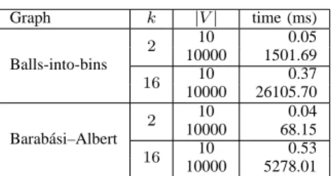
VI. EXPERIMENTAL ANALYSIS
In this Section, we report the results of our experimental study on the approximation algorithm given in Theorem 5.2 which is denoted by ALG in the remainder of the section.
The experiments have been carried out on a workstation equipped with a 2.66 GHz processor (Intel Core2 Duo E6700 Box) and 8Gb RAM running Linux 2.6 kernel and Gcc compiler, version 4.3.5.
We implemented algorithm ALG by using the LEMON
Graph Library [23] framework. In order to solve the IMCF
instances required by ALG we used the Network Simplex
algorithm [24] provided by LEMON as it is the most experi-mentally efficient in general cases.
A. Input data and executed tests.
Instances of MCFMI have been randomly generated by
using two different models: The balls-into-bins [25], [26] and the Barab´asi-Albert power-law [27] models.
The balls-into-bins model is used to simulate devices thrown at random in a two-dimensional space [25]. In this model, each
instance ofMCFMI is made of a graph GBIB= (VBIB, EBIB),
a set of interfaces IBIB = {1, 2, . . . , k} along with cost
and bandwidth functions cBIB, and bBIB, and two allocation functionsWBIB: VBIB → 2IBIB andXBIB: VBIB× VBIB→ 2IBIB.
First, nodes in VBIB are generated and a uniformly random position in a unit size square is associated to each of them. From the “balls-into-bins” theory [26], we know that throwing randomly n points in a unit square, the probability that no
nodes are inside a circle of diameter d =qγlog nn is smaller thann−γ
4, hence, forγ > 4 and large n, this probability is very low. Therefore, to generate edges and interfaces we proceed as follows. For each interfacei ∈ IBIB, the radiusri> 0 of the
circle covered by interfacei is generated uniformly at random
inh|V1 BIB|, q γlog(|VBIB|) |VBIB| − 1 |VBIB| i
. In this way, interfaces cover a circle having an average diameter of
q
γlog |VBIB|
|VBIB| . Then
func-tionWBIB is defined by independently assigning the generated interfaces to nodes with probability 0.5. Given two nodes u, v ∈ VBIB, let(xu, yu) and (xv, yv) be their associated
coor-dinates in the unit square. If p(xu− xv)2+ (yu− yv)2 ≤ ri, for some i ∈ WBIB(u) ∩ WBIB(v), an edge {u, v} is
added to EBIB and interface i is added to XBIB(u, v), i.e., XBIB(u, v) = WBIB(u) ∩ WBIB(v). In this way, for large values
of |VBIB| and γ > 4, we have a high probability to obtain a
connected network. Finally, functionscBIBandbBIBare defined as cBIB(i) = rα
i andbBIB(i) = r β
i, for eachi ∈ IBIB and for
suitable tuning parameterα, and β which are fixed to 1.5, and
2, respectively in the experiments. Source and target nodes are chosen as the nodes with the biggest Euclidean distance.
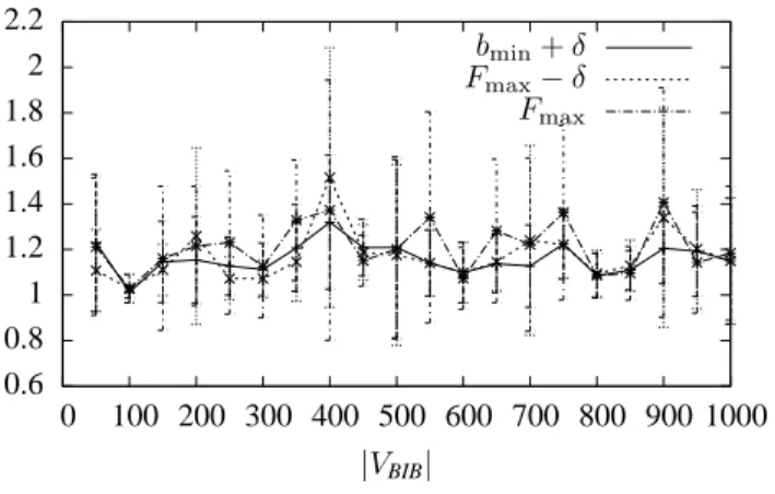
Barab´asi–Albert networks have been proven to model many real-world networks such as the Internet, the World Wide Web, citation graphs, and some social networks [28]. A Barab´asi– Albert topology is generated by iteratively adding one node at a time, starting from a given connected graph with at least two nodes. A newly added node is connected to any other existing nodes with a probability that is proportional to the degree that the existing nodes already have. Hence, the more connected a node is, the more likely it is to receive new connections to the new node. This mechanism is known as
preferential attachment and it has been observed in many
real-world networks.
In this model, each generated instance of MCFMI is
made of a graph GBA = (VBA, EBA), a set of interfaces IBA= {1, 2, . . . , k} along with cost and bandwidth functions cBA, and bBA, and two allocation functions WBA: VBA→ 2IBA
andXBA: VBA× VBA→ 2IBA. The graph generation algorithm
works as follows. We start from a graph made of two nodes connected by an edge and add one node at a time. A new node v is connected to an existing node u with probability p(v, u) = deg(u)2m , wheredeg(u) is the degree of node u before
addingv and m is the number of edges that already exist when v is added. Interfaces IBA and related costs and bandwidth functions are generated in a way similar to the balls-into-bins model, that is, for each interface i ∈ IBA, a number ri is
generated uniformly at random inh|V1
BA|, q γlog(|VBA|) |VBA| − 1 |VBA| i , thencBA(i) and bBA(i) are set to cBA(i) = rα
i andbBA(i) = r β i.
Parameters γ, α, and β are set to 5, 1.5, and 2, respectively.
TABLE II SIZE OF THE INPUT DATA.
Graph |V | k
Balls-into-bins {50, 100, . . . , 1000} {3, 6, 9}
{10, 100, 1000, 10000} {2, 4, . . . , 16}
Barab´asi–Albert {50, 100, . . . , 1000} {3, 6, 9}
{10, 100, 1000, 10000} {2, 4, . . . , 16}
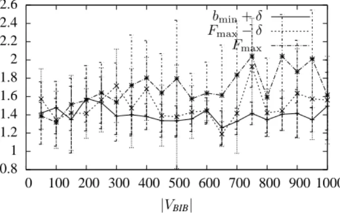
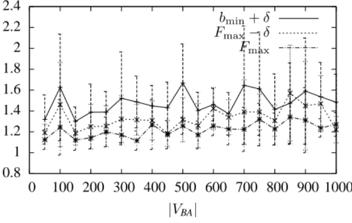
Fig. 5. Graphs GBIB: average upper bounds on the approximation ratios for
|VBIB| ∈ {50, 100, . . . , 1000}, k = 9 and three values of required flow.
Fmax Fmax− δ bmin+ δ |VBIB| 1000 900 800 700 600 500 400 300 200 100 0 2.6 2.4 2.2 2 1.8 1.6 1.4 1.2 1 0.8
For each edge {u, v} ∈ EBA, interface i ∈ IBA is added to
XBA(u, v) with probability 0.5. For each node v, WBA(v) is
induced by the interfaces associated inXBA(u, v) for each edge {u, v} incident to v. Source and target nodes are chosen at
random among the generated nodes.
For each of the defined instances in both the models above, we considered four values of required flow equally distributed between the minimal bandwidth assigned to an interfacebmin
and the maximum flow possible Fmax, computed by the
algorithm given in Theorem 4.1. That is, we required a flow ofbmin+ i ·Fmax3−bmin, fori = 0, 1, 2, 3. In the remainder, we
will not consider the case where the required flow isbmin(i.e. i = 0) as in this case we are able to find an optimal solution to MCFMI by computing a cheapest path (see [11]) connecting
source and destination. When the considered instance is clear by the context, we denote Fmax−bmin
3 simply byδ.
In order to measure the approximation ratio in the above settings, we need to know the optimal value of eachMCFMI
instance. As it is NP -hard to compute such value, we
mea-sured the ratio between the objective function value computed by our algorithm and a lower bound to the optimal value, obtaining an upper bound to the actual approximation ratio. In detail, we computed two lower bounds to the optimal value and then we use the maximum among them to get a better estimate of the approximation ratio. One lower bound is simply given by the optimal solution of theIMCF instance defined in ALG. Another lower bound to the optimal value is computed
by observing that, if we relax the bandwidth constraints by increasing the bandwidth of an interface, we decrease the optimal value. Hence, we computed a lower bound to the optimal value as the optimal value of an instance obtained by setting the bandwidth of each interface to the maximum bandwidth assigned to the original instance. Such a value can be polynomially computed by using Corollary 5.3.