Is the Market Portfolio Efficient? A New Test of Mean-Variance Efficiency when all Assets are Risky

HAL Id: hal-01493323

https://hal.archives-ouvertes.fr/hal-01493323

Submitted on 21 Mar 2017

HAL is a multi-disciplinary open access

archive for the deposit and dissemination of sci-entific research documents, whether they are pub-lished or not. The documents may come from teaching and research institutions in France or abroad, or from public or private research centers.

L’archive ouverte pluridisciplinaire HAL, est destinée au dépôt et à la diffusion de documents scientifiques de niveau recherche, publiés ou non, émanant des établissements d’enseignement et de recherche français ou étrangers, des laboratoires publics ou privés.

Is the Market Portfolio Efficient? A New Test of

Mean-Variance Efficiency when all Assets are Risky

Marie Brière, Bastien Drut, Valérie Mignon, Kim Oosterlinck, Ariane Szafarz

To cite this version:

Marie Brière, Bastien Drut, Valérie Mignon, Kim Oosterlinck, Ariane Szafarz. Is the Market Portfolio Efficient? A New Test of Mean-Variance Efficiency when all Assets are Risky. Finance, Presses universitaires de Grenoble, 2013, 34 (1), pp.7 - 41. �hal-01493323�

Is the Market Portfolio Efficient?

A New Test to Revisit the Roll (1977)

versus Levy and Roll (2010) Controversy

Université de Paris Ouest Nanterre La Défense (bâtiments T et G) 200, Avenue de la République 92001 NANTERRE CEDEX Tél et Fax : 33.(0)1.40.97.59.07 Email : nasam.zaroualete@u-paris10.fr

Document de Travail

Working Paper

2011-20

Marie Brière

Bastien Drut

Valérie Mignon

Kim Oosterlinck

Ariane Szafarz

E

c

o

n

o

m

i

X

http://economix.fr

7235

1

Is the Market Portfolio Efficient?

A New Test to Revisit the Roll (1977) versus Levy and

Roll (2010) Controversy

Marie Brière

Université Libre de Bruxelles, SBS-EM, Centre Emile Bernheim, Belgium.

Bastien Drut

Amundi Asset Management, France.

Université Libre de Bruxelles, SBS-EM, Centre Emile Bernheim, Belgium. EconomiX-CNRS, University of Paris-Ouest, France.

Valérie Mignon*

EconomiX-CNRS, University of Paris-Ouest, France. CEPII, 113 rue de Grenelle, 75007 Paris, France.

Kim Oosterlinck

Université Libre de Bruxelles, SBS-EM, Centre Emile Bernheim, Belgium.

Ariane Szafarz

Université Libre de Bruxelles, SBS-EM, Centre Emile Bernheim, Belgium. June 28, 2011

We are grateful to Dick Roll for stimulating discussions during his stay at the Université Libre de Bruxelles. We also thank Gopal Basak for his helpful comments on a previous version of this paper.

*Corresponding author: Email: valerie.mignon@u-paris10.fr. Phone: +33.1.40975860. Fax: +33.1.40977784, Address: EconomiX-CNRS, University of Paris Ouest, 200 avenue de la République, 92001 Nanterre, France.

2

Abstract

Levy and Roll (Review of Financial Studies, 2010) recently revived the debate related to the market portfolio’s efficiency, suggesting that it may be mean-variance efficient after all. This paper develops an alternative test of portfolio mean-variance efficiency based on the realistic assumption that all assets are risky. The test is based on the vertical distance of a portfolio from the efficient frontier. Monte Carlo simulations show that our test outperforms the previous mean-variance efficiency tests for large samples since it produces smaller size distortions for comparable power. Our empirical application to the U.S. equity market highlights that the market portfolio is not mean-variance efficient, and so invalidates the zero-beta CAPM.

Keywords: Efficient portfolio, mean-variance efficiency, efficiency test. JEL codes: G11, G12, C12.

3

1. Introduction

Testing the mean-variance (MV) efficiency of the market portfolio, or equivalently testing the validity of the Capital Asset Pricing Model (CAPM) of Sharpe (1964) and Lintner (1965), is a major task for financial econometricians. The debate on this issue dates back to the breakthrough theoretical contributions of Roll (1977) and Ross (1977) questioning the efficiency of the market portfolio. In the wake of these contributions, numerous empirical studies (Gibbons, 1982; Gibbons et al., 1989; MacKinlay and Richardson, 1991; among others) found that the market portfolio may indeed lie far away from the efficient frontier. Ironically, this debate was recently fuelled by Levy and Roll (2010), who published an article in the Review of Financial Studies entitled “The market portfolio may be mean-variance efficient after all”. Based on a new test, we take a fresh look at this issue with the ambition to arbitrate between the contradictory arguments of Roll (1977) and Levy and Roll (2010).

More generally, all portfolio managers are—or should be—faced with the issue of checking whether a given portfolio is optimal within a predefined investment universe. For this purpose, MV efficiency, as defined by Markowitz (1952, 1959), remains the key optimality concept. Currently, the econometric literature offers a wide variety of tests for MV efficiency. Most are

designed for universes that include a riskless asset.1 This represents a considerable constraint

when it comes to practical implementation. By contrast, this paper focuses on MV efficiency tests that allow all assets to be risky.

1 _{When the investment universe includes a riskless asset, the efficient frontier is a straight line, which makes the}

derivations far simpler (Gourieroux et al., 1997). Tests falling in this category have been proposed by Gibbons (1982), Jobson and Korkie (1982), and MacKinlay and Richardson (1991), among others. The test introduced by Gibbons et al. (1989) has since then become the standard. Michaud (1989) and Green and Hollifield (1992) discuss the limitations of this framework. Besides, MV efficiency tests must be distinguished from MV spanning tests, which examine whether the efficient frontier built from a given set of assets intersects the frontier resulting from a larger set (see De Roon and Nijman (2001) for a survey).

4

The assumption that all assets are risky is highly relevant given that riskless assets are no longer realistic in modern financial markets. The recent debt crisis has highlighted that even the supposedly safest assets, namely sovereign bonds issued by developed countries, are exposed to default risk. In the same way, the freezing of the money markets and the Lehman Brothers’ bankruptcy underlined the counterparty and liquidity risks associated with money market investments (Acharya et al., 2010; Bruche and Suarez, 2010; Krishnamurthy, 2010). Investors can thus meet severe restrictions on borrowing (Black, 1972), and the riskless borrowing rate can largely exceed the Treasury bill rate (Brennan, 1971). For all these reasons, MV efficiency is better tested without assuming the availability of a riskless asset.

Two broad classes of MV efficiency tests for risky-asset universes exist in the literature: likelihood-based tests and geometric tests. The likelihood-based tests are directly inspired by the formulation of the CAPM. While the riskless asset is needed to establish the original CAPM, further refinements by Black (1972) allow the riskless asset to be replaced by the zero-beta portfolio. To address the nonlinearities embedded in the Black CAPM, Gibbons (1982) builds a likelihood-ratio test statistic, for which Kandel (1984, 1986) derives the exact asymptotic chi-square distribution. However, because this test uses the Gauss-Newton algorithm, practical implementation turns out to be complex (Zhou, 1991). Moreover, Shanken (1985) shows that Gibbons’ (1982) test tends to over-reject MV efficiency in finite

samples.2 Levy and Roll (2010) (henceforth, LR) offer a novel likelihood-ratio test for MV

efficiency. This test is based on implicitly estimating the zero-beta rate by determining the

minimal changes to sample parameters that make a market proxy efficient.3

2 _{In reaction to these criticisms, several authors (Shanken, 1985, 1986; Zhou, 1991; Velu and Zhou, 1999;}

Beaulieu et al., 2008) provide lower and upper bounds to the test p-values.

3 _{Small variations in expected returns and volatilities may indeed lead to significant changes in the MV efficient}

5

On the other hand, the first geometric test of Basak, Jagannathan and Sun (2002) (henceforth, BJS) is based on the “horizontal distance” between the portfolio whose MV efficiency is in

question and its same-return counterpart on the MV efficient frontier.4 Unfortunately, some

portfolios lack such a counterpart (Gerard et al., 2007), which in turn limits the applicability of the BJS test. By contrast, the “vertical test” proposed in this paper circumvents this limitation. Indeed, the vertical inefficiency measure proposed by Kandel and Stambaugh (1995), Wang (1998), and Li et al. (2003), namely the difference between the portfolio’s expected return and the expected return of its same-variance counterpart on the MV efficient frontier, is well defined for any portfolio.

Our contribution is twofold. First, we define the vertical test statistic for MV efficiency, establish its asymptotic distribution, and compare its size and power performances to those of the LR and BJS tests through Monte Carlo simulations. While no clear hierarchy emerges for small samples, the vertical test outperforms its competitors for large samples as it exhibits equivalent power with a smaller size. Secondly, we re-examine the market portfolio MV efficiency using the three tests under review (LR, BJS and the vertical tests). Irrespectively of the number of stocks in the universe, we find that the market portfolio is never MV efficient according to both the BJS and the vertical tests. For the LR test, the conclusion depends on the value given to the coefficient α, which determines the relative weight assigned to sample mean changes against standard deviation changes. In other words, the LR test reaches no clear-cut and definitive conclusion regarding the market portfolio’s efficiency. Although still frail, the evidence points to the inefficiency of the market portfolio, supporting the Roll’s (1977) critique of the CAPM.

4 _{The null hypothesis is that the “horizontal distance” is zero. BJS derive the asymptotic distribution of this}

distance. Interestingly, the BJS test can be implemented with and without restrictions on short-selling. Besides, the BJS test can also be used to compare efficient frontiers (Ehling and Ramos, 2006; Drut, 2010).

6

The paper is organized as follows. Section 2 presents the vertical test and its asymptotic properties. Section 3 assesses the size and power of the vertical test and its two competitors. Section 4 tests the Black CAPM on the U.S. equity market. Section 5 concludes.

2. The Vertical Test of Mean-Variance Efficiency

Consider an investment universe composed of N primitive assets with stationary returns

characterized by a N-dimensional vectorR , withE(R) , and Cov(R). The tested

portfolio, P, is composed of primitive assets. Let r denote its return, with E(r) _and

2 )

(r 

Var .

Given a sample of returns of size T denoted (R_t)_{t1..T for the N primitive assets and}(r_t)_t1..T

for portfolio P, the empirical counterparts of parameters ,  , , and _{ are respectively} 2

given by:









whereR and _t r are the date-t returns on the N primitive assets and on portfolio P, respectively. _t

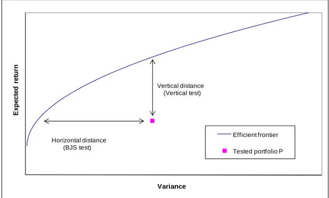
As illustrated by Figure 1, the “horizontal distance” underlying the BJS test measures of portfolio P inefficiency is the difference between the variance of P and the variance of its same-expected-return counterpart on the efficient frontier.

7

Figure 1. Horizontal and vertical distances between portfolio P and the efficient frontier

E x p ect ed r e tu rn Variance Efficient frontier Tested portfolio P Horizontal distance (BJS test) Vertical distance (Vertical test)

Our vertical test is conceived by transposing the BJS (2002) methodology to the vertical inefficiency measure introduced by Kandel and Stambaugh (1995), Wang (1998), and Li et al.

(2003). Hence, the vertical test statistic5 is the distance between the expected return of

portfolio P and the expected return of its same-variance MV efficient counterpart. The

estimated distance, denoted by ˆ , is the solution to the following program:







5 _{Another possibility would be to take the minimal Euclidian distance between portfolio P and the efficient}

frontier. This approach would certainly be more elegant, but would also be much more tedious as it would mix up first and second order parameters.

8

The following proposition states that, under the null that portfolio P is MV efficient, estimator

ˆ asymptotically follows a normal distribution:

Proposition 1

ˆ asymptotically follows a normal distribution:

T(ˆ) N(0,2) as T . (6) with                    V V   2 _{, where}

represents the asymptotic covariance matrix of the distinct elements of ˆ, ˆ, ˆ, and ˆ , and 

       V 

is given by (A2) in Appendix A.

Proof: See Appendix A.

As for the BJS test, this asymptotic result does not require normality assumptions on the asset returns. Moreover, as demonstrated in Appendix A, this result holds both with and without short-selling restrictions.

3. Power and Size Performances

In this section, we assess the size and power of the vertical test and compare its performances to those of the BJS and LR tests. To this end, we simulate series of returns drawn from the investment universe imagined by Das et al. (2010), including three assets with jointly normal returns having the following parameters:

           25 . 0 10 . 0 05 . 0              2500 . 0 0200 . 0 0000 . 0 0200 . 0 0400 . 0 0000 . 0 0000 . 0 0000 . 0 0025 . 0 (8)

9

Das et al. (2010) interpret the first asset as a bond, the second as a low-risk stock, and the

third as a highly speculative stock. For the sake of comparability,6 we focus here on the case

where short-selling is allowed.

We simulated 1,000 series of returns of lengths 60, 120, 180, and 240, respectively. In each case, two groups of portfolios were composed. The portfolios in the first group were generated on the efficient frontier in order to estimate the risk of type I error (false rejection of the true hypothesis that portfolios are mean-variance efficient). The portfolios in the second group were generated below the efficient frontier to estimate the risk of type II error (failure to reject the false hypothesis).

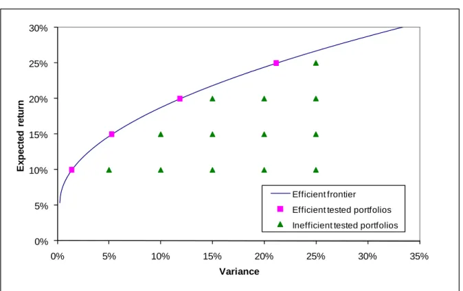
We follow the assessment of statistical tests suggested by Wasserman (2004). This procedure is based on power maximization (i.e., minimization of the risk of type II error) for a given small size (i.e., risk of type I error). Figure 2 features all tested portfolios on a grid in the MV plane. To each of them, we successively apply the BJS, LR, and vertical tests.

6 _{LR solely apply their test to cases where short-selling is allowed. Actually, the performances of their test when}

10

Figure 2. Efficient frontier and tested portfolios

0% 5% 10% 15% 20% 25% 30% 0% 5% 10% 15% 20% 25% 30% 35% E x p ect ed r e tu rn Variance Efficient frontier

Efficient tested portfolios Inefficient tested portfolios

BJS (2002) measure the difference in variances  between the tested portfolio P and its MV

efficient counterpart with same expected return. The estimated horizontal distance is the solution to the following program:







Under the null that portfolio P is MV efficient, ˆ asymptotically follows a normal

distribution: _{T }ˆ_N(0,_2) _{as T .}

The Levy and Roll (2010) test draws on the evidence that slight variations in the sample parameters may make a portfolio MV efficient. More precisely, the LR test statistic is built

11

from asset-return parameters





parameters













 





where distance d is defined by:



 











and  _{is a coefficient determining the relative weight assigned to deviations in means relative}

to the deviations in standard deviations.7

For simplicity, Levy and Roll (2010) reduce the number of parameters to estimate by

imposing that covariance matrix * computed from (*,*) is based on the sample

correlation matrix:                                   N N C * 0 0 0 * 0 0 * ˆ * 0 0 0 * 0 0 * * 2 1 2 1                 (11)

Where Cˆ is the sample correlation matrix. In that way, only the variances have to be

estimated.

Under the hypothesis that the N original assets follow a jointly normal distribution, the likelihood ratio is given by:















12

This test statistic asymptotically follows a chi-square distribution with N2 degrees of freedom.

The choice of the trade-off parameter  in Equation (10) is instrumental to the

implementation of the LR test. Indeed, a low (resp. high) value of would create a bias

towards standard deviations (resp. means). In extreme cases (  0 and   1 ), the

asymptotic distribution of the LR test statistic degenerates into a chi-square with N degrees of freedom. In our performance assessments, we follow Levy and Roll (2010) and set the value of α to 0.75.

3.1. False Rejection of Efficient Portfolios

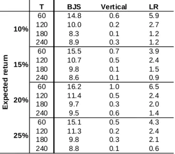
We first assess the type I error. The four simulated efficient portfolios have expected returns of 10%, 15%, 20% and 25%, respectively. The rejection frequencies of the null of portfolio

efficiency at the 5% probability level are displayed in Table 1.8 The results show that the size

is uniformly the lowest for the vertical test, followed by the LR test. Nevertheless, the vertical test, and to a lesser extent the LR test, exhibit rejection frequencies that lie below the theoretical threshold of 5%.

13

Table 1. Rejection frequencies (in percent) at the 5% probability level for the efficient portfolios T BJS Vertical LR 60 7.6 0.6 3.7 120 5.5 0.4 1.8 180 5.1 0.4 1.4 240 4.1 0.2 1.3 60 6.1 0.6 2.9 120 6.4 0.4 1.9 180 5.1 0.0 1.3 240 4.6 0.0 1.5 60 8.6 0.6 3.1 120 5.8 0.4 1.7 180 5.4 0.3 1.5 240 4.6 0.2 1.6 60 6.4 0.6 2.8 120 6.3 0.4 1.7 180 5.6 0.0 1.5 240 4.9 0.0 0.0 10% 15% 20% 25% Ex p e c te d r e tu rn

Note: BJS: Basak et al. (2002) test; Vertical: vertical test; LR: Levy and Roll (2010) test. T is the sample size.

3.2. Rejection of Inefficient Portfolios

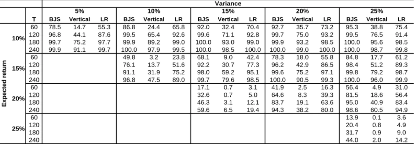
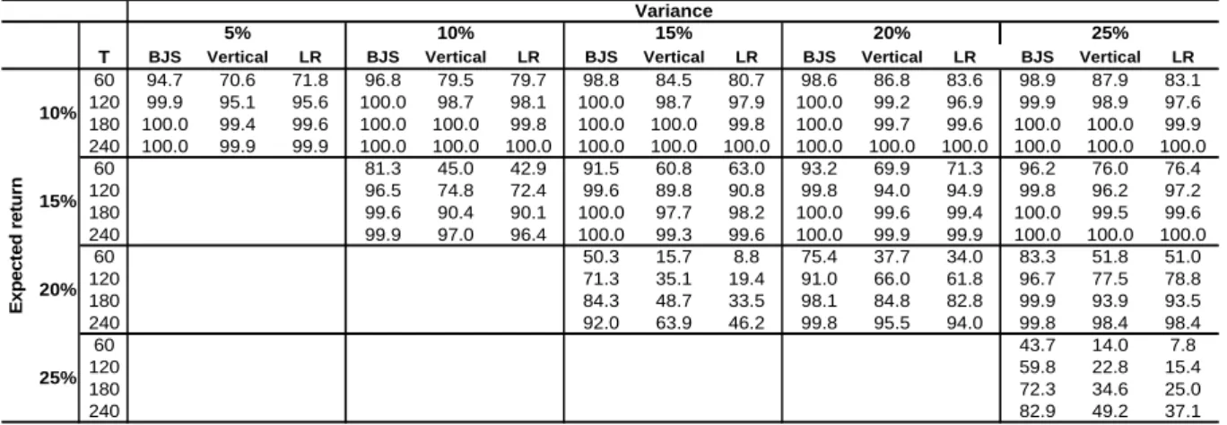
We now apply the three MV efficiency tests under review to thirteen portfolios simulated as inefficient in order to assess the probability of falsely concluding that the portfolio was

efficient. The results are given in Table 2 for 5% probability.9

9 _{The results corresponding to the 1% and 10% probability levels are given in Tables B2 and B3 in Appendix B,}

14

Table 2. Rejection frequencies (in percent) at the 5% probability level for the inefficient portfolios

T BJS Vertical LR BJS Vertical LR BJS Vertical LR BJS Vertical LR BJS Vertical LR

60 89.8 49.1 66.6 94.4 62.0 76.4 96.8 69.0 76.7 96.8 70.3 79.9 98.2 72.3 80.6 120 99.2 85.4 93.9 100.0 93.4 96.4 100.0 94.7 96.2 100.0 96.6 95.9 99.7 96.4 96.1 180 100.0 96.7 99.1 100.0 98.9 99.6 100.0 99.5 99.7 100.0 99.3 99.3 100.0 99.9 99.4 240 100.0 99.5 99.9 100.0 99.7 100.0 100.0 100.0 100.0 100.0 100.0 100.0 100.0 100.0 99.9 60 71.5 24.8 35.1 86.5 38.0 55.4 89.4 49.9 66.7 93.8 55.4 72.3 120 92.1 51.7 64.5 98.5 72.6 87.2 99.1 83.1 92.5 99.7 86.8 94.9 180 98.8 75.3 86.5 99.6 92.7 97.4 100.0 96.2 98.9 100.0 97.6 99.5 240 99.8 88.9 93.8 100.0 97.9 99.5 100.0 99.2 99.9 100.0 99.7 99.9 60 35.6 5.2 5.9 64.5 19.2 27.2 75.7 28.5 44.6 120 56.3 12.9 12.2 84.2 41.7 53.0 93.8 56.3 71.6 180 73.6 25.8 24.8 95.7 67.1 75.6 99.5 81.4 90.5 240 83.8 38.1 36.6 99.0 82.0 89.9 99.8 93.0 97.0 60 31.9 3.3 5.6 120 44.6 9.2 11.5 180 58.2 14.7 19.0 240 72.0 24.0 28.6 Ex p e c te d r e tu rn 10% 15% 20% 25% 15% 20% 25% Variance 5% 10%

Note: BJS: Basak et al. (2002) test; Vertical: vertical test; LR: Levy and Roll (2010) test. T is the sample size.

For sample sizes below 180, the power is the lowest for the vertical test, and the highest for the BJS test. However, for larger samples, the vertical test outperforms both the BJS and the LR tests since its size is the lowest for an equivalent power. On the whole, Tables 1 and 2 indicate that the vertical test rejects the null of MV efficiency less frequently than the two other tests.

The differences in power and size between the vertical test and the BJS test might look surprising since both are similar in spirit, namely they are both built from a geometric one-dimensional measure of inefficiency in the MV plane. This counterintuitive result stems from the fact that the standard deviation of the vertical measure of inefficiency is higher than the standard deviation of the horizontal measure used in the BJS test. Indeed, the standard deviations of both tests depend on the absolute values of the weighting loads of the tested-portfolio efficient counterpart. However, the efficient “vertical counterparts” are mostly located on the top of the efficient frontier while the efficient “horizontal counterparts” are mostly located at the bottom of the efficient frontier. Since absolute weighting loads are typically higher on the top of the efficient frontier (riskier portfolios are less diversified), the

15

vertical distance is subject to higher standard deviations than the horizontal BJS test. Consequently, the t-statistic generally takes lower values for the vertical test than for the BJS test, and hence the former rejects MV efficiency less frequently than the latter. This feature is particularly relevant when short-selling restrictions are imposed (see Best and Grauer, 1991; Green and Hollifield, 1992; Britten-Jones, 1999).

3.3. Robustness Checks on the Slope of the Efficient Frontier

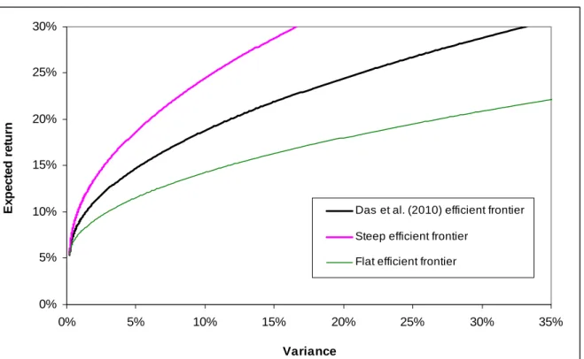
Both the horizontal and vertical measures of portfolio inefficiency are restricted to a single dimension in the MV plane. They are, therefore, sensitive to the slope of the efficient frontier. For this reason, we check the robustness of our previous findings by substantially modifying the slope of the efficient frontier. This is achieved by running simulations under two alternative scenarios for the expected return on the speculative stock (15% and 35% respectively instead of 25%) while keeping all other parameters in Equation (8) unchanged. As Figure 3 shows, the first case (15%) produces a flatter efficient frontier, whereas the second (35%) leads to a steeper MV efficient frontier. The minimum-variance portfolios of the three efficient frontiers still remain very close to each other. As previously, we apply the three efficiency tests to a grid of efficient and non-efficient simulated portfolios.

16

Figure 3. The three efficient frontiers under consideration

0% 5% 10% 15% 20% 25% 30% 0% 5% 10% 15% 20% 25% 30% 35% Variance E x p ected r e tu rn

Das et al. (2010) efficient frontier Steep efficient frontier

Flat efficient frontier

The results are reported in Tables C1 to C4 in Appendix C. They can be summarized as follows. For the flat efficient frontier, the BJS test produces the highest size distortions, while the vertical test exhibits the lowest. Given that the BJS test outperforms the other two tests in terms of power irrespective of the sample size, a reasonable procedure for practical use is to combine the BJS and the vertical tests when the MV efficient frontier is flat. In the case of a steep efficient frontier, the results are similar to those obtained in the benchmark case. The vertical test exhibits the lowest size distortions, and its power strongly increases in comparison to the benchmark case, especially for small samples. On the whole, our results show that the vertical test is preferable when the efficient frontier is steep and samples are large.

17

4. Is the Market Portfolio Efficient?

In this section, we apply the BJS, the LR,and the vertical tests of MV efficiency to the

capitalization-weighted market portfolio made up of the 100 largest U.S. stocks10 by market

capitalizations as measured on December 31, 2010. The data are monthly returns over the period January 1988 – December 2010 (276 observations). To gauge the sensitivity of our

results with respect to the number of available stocks, 11 we also run the tests in stock

universes of different sizes (N 10,20,_,100).12 In each case, we select the largest stocks of

the sample. For the LR test we follow the original paper when assessing MV efficiency and use a value of α equal to 0.75. As a robustness check, we also test the MV efficiency for a

value α (0.98), which gives a similar importance to deviations from variance and mean.13

Lastly, we apply the three tests to equally-weighted portfolios as robustness checks.

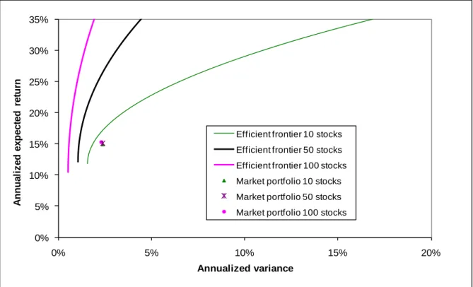
Figure 4 shows the efficient frontiers (without short-selling restrictions) made of 10, 50 and 100 assets, respectively, and the corresponding market portfolios. Noticeably, the MV characteristics of the market portfolio are stable with respect to the number of assets, but the efficient frontier becomes steeper when N increases. In particular, this feature shows that all configurations explored in Section 3 are realistic.

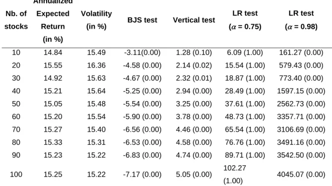
Table 3 summarizes the outcomes of the three tests. Two findings stand out. Firstly, for all sample sizes, both the BJS and the vertical tests reject the null of market portfolio efficiency.

10 _{We selected the 100 largest stocks of the S&P 500 index.}

11 _{The data are extracted from the Datastream database. Descriptive statistics are given in Appendix D.}

12 _{In reality, individual investors rarely hold portfolios containing 100 assets (Barber and Odean, 2000;}

Polkovnichenko, 2005; Goetzmann and Kumar, 2008). The diversification benefits tend to be exhausted once an equity portfolio contains several tens of stocks (Evans and Archer, 1968; Elton and Gruber, 1977; Statman, 1987).

13 _{This value is actually very close to the 0.98-value considered in LR as more realistic than the 0.75 used to test}

18

Regardless of the number of stocks in the universe, the market portfolio is never MV efficient. Similar results are found for equally-weighted portfolios (see Table 4).

Secondly, for all values of N, the LR test does not reject market portfolio efficiency for α =

0.75, confirming the findings of Levy and Roll (2010).14 _{However, for α = 0.98 the LR test}

rejects market portfolio efficiency. This indicates that the LR test is sensitive to the value taken by parameter α. In fact, for α higher than 0.902 MV efficiency is always rejected by the LR test.

Figure 4. Efficient frontiers and market portfolios for the 10, 50 and 100 largest U.S. stocks, respectively. January 1988 – December 2010

0% 5% 10% 15% 20% 25% 30% 35% 0% 5% 10% 15% 20% A nnua li z e d e x pe c te d r e tu rn Annualized variance

Efficient frontier 10 stocks Efficient frontier 50 stocks Efficient frontier 100 stocks Market portfolio 10 stocks Market portfolio 50 stocks Market portfolio 100 stocks

19

Table 3. MV efficiency tests for the capitalization-weighted market portfolio

Nb. of stocks Annualized Expected Return (in %) Volatility

(in %) BJS test Vertical test

LR test ( = 0.75) LR test ( = 0.98) 10 14.84 15.49 -3.11(0.00) 1.28 (0.10) 6.09 (1.00) 161.27 (0.00) 20 15.55 16.36 -4.58 (0.00) 2.14 (0.02) 15.54 (1.00) 579.43 (0.00) 30 14.92 15.63 -4.67 (0.00) 2.32 (0.01) 18.87 (1.00) 773.40 (0.00) 40 15.21 15.64 -5.25 (0.00) 2.94 (0.00) 28.49 (1.00) 1597.15 (0.00) 50 15.05 15.48 -5.54 (0.00) 3.25 (0.00) 37.61 (1.00) 2562.73 (0.00) 60 15.20 15.54 -5.90 (0.00) 3.78 (0.00) 48.73 (1.00) 3357.71 (0.00) 70 15.27 15.40 -6.56 (0.00) 4.46 (0.00) 65.54 (1.00) 3106.69 (0.00) 80 15.33 15.31 -6.53 (0.00) 4.58 (0.00) 76.76 (1.00) 3491.16 (0.00) 90 15.23 15.22 -6.83 (0.00) 4.74 (0.00) 89.71 (1.00) 3542.50 (0.00) 100 15.25 15.22 -7.17 (0.00) 5.05 (0.00) 102.27 (1.00) 4045.07 (0.00) Coefficient  denotes the MV trade-off in the LR test statistic. p-values are given in parentheses.

Table 4. MV efficiency tests for the equally-weighted market portfolio

Nb. of stocks Annualized Expected Returns (in %) Volatility

(in %) BJS test Vertical test

LR test ( = 0.75) LR test ( = 0.98) 10 14.29 14.95 -3.22 (0.00) 1.33 (0.09) 6.78 (1.00) 197.70 (0.00) 20 15.34 16.79 -4.56 (0.00) 2.18 (0.01) 15.75 (1.00) 706.71 (0.00) 30 14.32 15.50 -4.54 (0.00) 2.39 (0.01) 19.37 (1.00) 979.52 (0.00) 40 15.17 15.72 -4.99 (0.00) 2.90 (0.00) 28.48 (1.00) 1771.03 (0.00) 50 14.79 15.47 -5.27 (0.00) 3.23 (0.00) 36.90 (1.00) 2681.93 (0.00) 60 15.22 15.76 -5.65 (0.00) 3.75 (0.00) 47.80 (1.00) 3381.66 (0.00) 70 15.39 15.46 -6.14 (0.00) 4.36 (0.00) 64.71 (1.00) 3453.09 (0.00) 80 15.53 15.28 -6.00 (0.00) 4.45 (0.00) 75.95 (1.00) 3938.86 (0.00) 90 15.21 15.13 -6.29 (0.00) 4.60 (0.00) 89.03 (1.00) 4137.95 (0.00) 100 15.30 15.17 -6.68 (0.00) 4.92 (0.00) 102.12 (1.00) 4535.09 (0.00) Coefficient  denotes the MV trade-off in the LR test statistic. p-values are given in parentheses.

On the whole, our findings support Roll (1977) over Levy and Roll (2010). Indeed, while the

20

unequivocally conclude that the market portfolio is never MV efficient. The validity of the zero-beta CAPM, relying on the efficiency of the market portfolio, is thus strongly called into question. In a nutshell, the fundamental contributions of both Roll (1977) and Ross (1977) remain highly relevant for portfolio management.

5. Conclusion

This paper develops a new test of portfolio MV efficiency based on the realistic assumption that all assets are risky. The test is based upon the vertical distance of a portfolio from the efficient frontier. While the evidence is mixed for small samples, our test outperforms the previous MV efficiency tests proposed by Basak et al. (2002) and Levy and Roll (2010) for large samples since it produces lower size distortions for comparable power. The empirical analysis shows that the LR test is sensitive to the value taken by the nuisance parameter determining the relative weight assigned to sample-mean changes against standard-deviation changes. Furthermore, both the vertical and horizontal tests are based on intuitive measures in the MV plane and are, therefore, easy to visualize, which makes them more appealing than the LR test.

The ideally balanced distance in the MV plane remains, however, the orthogonal distance. Even though a test based on this distance is feasible in theory, deriving its closed-form asymptotics could prove challenging. We leave this for further work. Meanwhile, the best alternative for practitioners to test portfolio efficiency is probably the dual approach combining the vertical and horizontal tests. In the final decision, the weight to be allocated to each test should then take into account the curvature of the efficient frontier.

21

The existing MV efficiency tests could be improved in several ways. The LR test could be generalized by relaxing the short-selling restriction. For all tests, implementing the jackknife-type estimator of the covariance matrix developed by Basak et al. (2009) could offer a promising extension since this estimator produces a more accurate covariance matrix than the sample one.

Our empirical application to the U.S. equity market highlights that the market portfolio is not MV efficient, invalidating the zero-beta CAPM. Consequently, regarding the Roll (1977) versus Levy and Roll (2010) controversy, our findings indicate that Roll’s (1977) scepticism on the validity of the CAPM seems to survive the recent rehabilitation attempts made by Levy and Roll (2010).

22

References

Acharya, V.V., D.M. Gale and T. Yorulmazer. 2011. Rollover Risk and Market Freezes. Journal of Finance, forthcoming.

Barber, B.M. and T. Odean. 2000. Trading Is Hazardous to Your Wealth: The Common Stock Investment Performance of Individual Investors. Journal of Finance 55:773-806.

Basak, G., R. Jagannathan, and G. Sun. 2002. A Direct Test for the Mean-Variance Efficiency of a Portfolio. Journal of Economic Dynamics and Control 26:1195-1215.

Basak, G., R. Jagannathan, and T. Ma. 2009. Jackknife Estimator for Tracking Errors Variance of Optimal Portfolios. Management Science 55:990-1002.

Beaulieu, M.-C., J.-M. Dufour and L. Khalaf. 2008. Finite Sample Identification-Robust Inference for Unobservable Zero-Beta Rates and Portfolio Efficiency with Non-Gaussian Distributions. Technical report, Mc Gill University, Université Laval and Carleton University. Best, M.J. and R.R. Grauer. 1991. On the Sensitivity of Mean-Variance Efficient Portfolios to Changes in Asset Means: Some Analytical and Computational Results. Review of Financial Studies 4:315-342.

Black, F. 1972. Capital Market Equilibrium with Restricted Borrowing. Journal of Business 45:444-454.

Brennan, M. 1971. Capital Market Equilibrium with Divergent Borrowing and Lending Rates. Journal of Financial and Quantitative Analysis 6:1197-1205.

Britten-Jones, M.J. 1999. The Sampling Error in Estimates of Mean-Variance Efficient Portfolio Weights. Journal of Finance 54:655-671.

Bruche, M. and J. Suarez. 2010. Deposit Insurance and Money Market Freezes. Journal of Monetary Economics 57:45-61.

Das, S., H. Markowitz, J. Scheid and M. Statman. 2010. Portfolio Optimization with Mental Accounts. Journal of Financial and Quantitative Analysis 45:311-334.

De Roon, F.A. and T.E. Nijman. 2001. Testing for Mean-Variance Spanning: A Survey. Journal of Empirical Finance 8:111-155.

Drut, B. 2010. Sovereign Bonds and Socially Responsible Investment. Journal of Business Ethics 92:131-145.

Ehling, P. and S.B. Ramos. 2006. Geographic versus Industry Diversification: Constraints Matter. Journal of Empirical Finance 13:396-416.

Elton, E.J. and M.J. Gruber. 1977. Risk Reduction and Portfolio Size: An Analytical Solution. Journal of Business 50:415-437.

23

Evans, J.L. and S.H. Archer. 1968. Diversification and the Reduction of Dispersion: An Empirical Analysis. Journal of Finance 23:761-767.

Gerard, B., P. Hillion, F.A. de Roon, and E. Eiling. 2007. International Portfolio Diversification: Currency, Industry and Country Effects Revisited. Working paper available at

doi:10.2139/ssrn.302353.

Gibbons, M.R. 1982. Multivariate Tests of Financial Models: A New Approach. Journal of Financial Economics 10:3-27.

Gibbons, M.R., S.A. Ross and J. Shanken. 1989. A Test of the Efficiency of a Given Portfolio. Econometrica 57:1121-1152.

Goetzmann, W.N. and A. Kumar. 2008. Equity Portfolio Diversification. Review of Finance, 12:433-463.

Gourieroux, C., O. Scaillet, and A. Szafarz. 1997. Econométrie de la Finance : Approches Historiques. Paris: Economica.

Green, R.C. and B. Hollifield. 1992. When Will Mean-Variance Efficient Portfolios Be Well Diversified? Journal of Finance 47:1785-1809.

Jobson, J.D. and B. Korkie. 1982. Potential Performance and Tests of Portfolio Efficiency. Journal of Financial Economics 10:433-466.

Kandel, S. 1984. The Likelihood Ratio Test Statistic of Mean-Variance Efficiency without a Riskless Asset. Journal of Financial Economics 13:575-592.

Kandel, S. 1986. The Geometry of the Likelihood Estimator of the Zero-Beta Return. Journal of Finance 41:339-346.

Kandel, S. and R.F. Stambaugh. 1995. Portfolio Inefficiency and the Cross-Section of Expected Returns. Journal of Finance 50:157-184.

Krishnamurthy, A. 2010. The Financial Meltdown: Data and Diagnoses. Working Paper, Northwestern University.

Levy, M. and R. Roll. 2010. The Market Portfolio May Be Mean/Variance Efficient After All. Review of Financial Studies 23:2464-2491.

Li, K., S. Asani and Z. Wang. 2003. Diversification Benefits of Emerging Markets Subject to Portfolio Constraints. Journal of Empirical Finance 10:57-80.

Lintner, J. 1965. Security Prices, Risk, and the Maximal Gains from Diversification. Journal of Finance 20:587-615.

MacKinlay, A.C. and M.P. Richardson. 1991. Using Generalized Method of Moments to Test Mean-Variance Efficiency. Journal of Finance 46:511-527.

24

Markowitz, H. 1952. Portfolio Selection. Journal of Finance 7:77-91.

Markowitz, H. 1959. Portfolio Selection: Efficient Diversification of Investments. New York: John Wiley.

Michaud, R.O. 1989. The Markowitz Optimization Enigma: Is ‘Optimized’ Optimal? Financial Analysts Journal 45:31-42.

Polkovnichenko, V. 2005. Household Portfolio Diversification: A Case for Rank-Dependent Preferences. Review of Financial Studies 18:1467-1502.

Roll, R. 1977. A Critique of the Asset Pricing Theory’s Tests. Part I: On Past and Potential Testability of the Theory. Journal of Financial Economics 4:129-176.

Ross, S.A. 1977. The Capital Asset Pricing Model (CAPM), Short-Sale Restrictions and Related Issues. Journal of Finance 19:425-442.

Shanken, J. 1985. Multivariate Tests of the Zero-Beta CAPM. Journal of Financial Economics 14:327-348.

Shanken, J. 1986. Testing Portfolio Efficiency when the Zero-Beta Rate is Unknown: A Note. Journal of Finance 41:269-276.

Sharpe, W.F. 1964. Capital Asset Prices: A Theory of Market Equilibrium under Conditions of Risk. Journal of Finance 19:425-442.

Statman, M. 1987. How Many Stocks Make a Diversified Portfolio? Journal of Financial and Quantitative Analysis 22:353-363.

Velu, R. and G. Zhou. 1999. Testing Multi-Beta Asset Pricing Models. Journal of Empirical Finance 6:219-241.

Wang, Z. 1998. Efficiency Loss and Constraints on Portfolio Holdings. Journal of Financial Economics 48:359-375.

Wasserman, L. 2004. All of Statistics: A Concise Course in Statistical Inference. New York: Springer.

Zhou, G. 1991. Small Sample Tests of Portfolio Efficiency. Journal of Financial Economics 30:165-191.

25

Appendix A: Proof of Proposition 1

We first derive the asymptotic distribution of the vertical distance, ˆ , defined in Equation (5)

in the case where short-selling is forbidden. At the end of this Appendix, we extend the results to the case where short-selling is allowed

Let x be a k-dimensional vector, and denote ( , 1,..., )'

) ( k i i i x x x x   . Consider a symmetric

matrix B of order k, and B[B₁:B₂:...:B_k]whereB is the _{i i}th_{column of B. Let vec(B) be}

the stacked vector of the columns of B:

)' , , , ( ) ( (2)' ( )' 2 )' 1 ( 1 k k B B B B vec  _

Next, let V be the vector formed by stacking the sample mean of R , the elements of _t

)

cov(R , the sample mean of _t r , and the sample variance of _t r : _t ²)' ˆ , ˆ , ))' ˆ ( ( ,' ˆ (     vec V

Vector V thus summarizes the first and second moments of the sample returns. Similarly to

BJS (2002), we express vector V as a function of the sample non-central first and second

moments of _{R and t} r . The transformed vector, _t U , is defined by: _t

)' , ,' , ( )' , , ))' ' ( ( , ( ' 2 ' t t t t t t t t t t R vec R R r r R Y r w U  

and its sample mean,U , is:





Let g(.)denote the function that maps vector U to vector V :

V vec w vec Y w Y g U g                                                  ² ˆ ˆ ) ˆ ( ˆ ² ˆ ˆ ) ' ˆ ˆ ( ˆ ˆ ˆ ) (          

26









D and  being the covariance matrix of ₀ U , and from BJS (2002, p. 1208): _t

                                         1 : ˆ 2 0 : 1 0 0 0 0 0 2 2 2 1 2  pv p p pv pv p pv p p U x K I K I x g D T  (A3) Where ( 1) 2 p p pv  ;









for the ith element of ˆ, and I stands for the identity matrix of rank Z. _Z

The asymptotic distribution of vector V is given by (A1). Let us now move to the vertical

distance, ˆ , which is a derivable function of vector V . Consequently, the delta method

establishes that the asymptotic variance _2 _{of }ˆ _is

                      V V  ˆ ˆ , where derivative V  ˆ

needs to be computed. With this aim, we express that ˆ minimizes the following Lagrangian

function:            ˆ ' ˆ ( ' 1) ( 'ˆ ˆ2) ' 2 1         l (A4) By differentiation, we have: V V l V              _{    }  ) ˆ ' 2 ' ' ' ˆ ( ˆ 2 1









27

From the first order condition applied to (A4), we obtain:

) ˆ 2 ( ' ˆ 0 ₁  ₁ ₂            v l p And consequently:









Combining the results in (A1), (A4) and (A6), we obtain the asymptotic variance _2_{of the}

vertical distance ˆ : _                      V V   2 ˆ ˆ (A7)

When there are no short-selling restrictions, the efficient frontier is modified because the sole

constraint applied tois that its components add up to one. Let ˆ* _{denote the vertical}

distance in this case. The modified Lagrangian function is:

* ˆ ' ˆ ( ' 1) ( 'ˆ ˆ2) 2 1                 l (A8)

By differentiating both sides of (A7), we get:









from (A5) gives the asymptotic variance _2*_{of the}

vertical distance ˆ* when there are no short-selling restrictions. Its expression stands as:

                       V V * ˆ * ˆ * 2    (A10)

28

Appendix B: Rejection Frequencies at the 1% and 10% Probability Levels

Table B1. Rejection frequencies (in percent) at the 1% and 10% probability levels for the efficient portfolios

T BJS Vertical LR BJS Vertical LR 60 1.7 0.0 2.2 16.7 2.2 4.7 120 0.9 0.0 0.6 12.3 1.3 3.0 180 0.6 0.0 0.7 12.8 1.3 2.6 240 0.5 0.0 0.4 11.2 1.2 2.1 60 2.2 0.0 1.7 13.6 2.3 4.0 120 1.6 0.0 0.7 14.2 1.5 2.7 180 1.3 0.0 0.5 12.4 1.6 2.3 240 0.9 0.0 0.4 12.1 1.0 1.8 60 2.4 0.0 1.7 17.8 2.3 4.1 120 1.0 0.0 0.6 14.5 1.3 2.9 180 0.8 0.0 0.6 13.7 1.3 2.3 240 0.8 0.0 0.4 12.1 1.2 2.1 60 2.2 0.0 1.4 14.1 2.4 4.1 120 1.5 0.0 0.7 14.3 1.6 2.9 180 1.3 0.0 0.5 12.5 1.4 2.2 240 0.9 0.0 0.0 12.2 1.1 0.0 Exp ect ed ret u rn 25% 10% 15% 20%

1% probability error 10% probability error

Note: BJS: Basak et al. (2002) test; Vertical: vertical test; LR: Levy and Roll (2010) test. T denotes the sample size.

Table B2. Rejection frequencies (in percent) at the 1% probability level for the inefficient portfolios

T BJS Vertical LR BJS Vertical LR BJS Vertical LR BJS Vertical LR BJS Vertical LR

60 78.5 14.7 55.3 86.8 24.4 65.8 92.0 32.4 70.4 92.7 35.7 73.2 95.3 38.8 75.4 120 96.8 44.1 87.6 99.5 65.4 92.6 99.6 71.1 92.8 99.7 75.0 93.2 99.5 76.5 91.4 180 99.7 75.2 97.7 99.9 89.2 99.0 100.0 93.0 99.0 99.9 93.2 98.5 100.0 95.6 98.5 240 99.9 91.1 99.7 100.0 97.9 99.5 100.0 98.5 100.0 100.0 99.0 100.0 100.0 98.7 99.8 60 49.8 3.2 23.8 68.1 9.0 42.4 78.3 18.0 55.8 84.8 17.7 61.2 120 76.1 13.7 51.6 92.2 30.7 77.3 96.2 42.9 86.5 98.4 51.2 89.3 180 91.1 31.9 75.2 98.0 59.2 95.1 99.6 75.2 97.1 99.8 79.2 98.7 240 96.8 47.5 89.0 99.7 79.6 98.5 100.0 90.5 99.3 100.0 96.0 99.9 60 17.1 0.7 3.1 41.9 2.5 16.3 56.4 4.9 31.0 120 32.6 0.7 5.0 64.6 8.3 39.3 81.5 18.6 56.4 180 46.3 3.1 12.1 83.7 19.1 63.6 95.0 40.9 83.4 240 59.6 6.5 19.4 94.3 38.2 80.0 98.6 60.5 94.9 60 13.9 0.1 3.6 120 20.4 0.8 4.9 180 31.7 0.9 9.0 240 44.0 2.0 14.2 Ex pec ted r e tu rn 10% 15% 20% 25% Variance 5% 10% 15% 20% 25%

Note: BJS: Basak et al. (2002) test; Vertical: vertical test; LR: Levy and Roll (2010) test. T denotes the sample size.

29

Table B3. Rejection frequencies (in percent) at the 10% probability level for the inefficient portfolios

T BJS Vertical LR BJS Vertical LR BJS Vertical LR BJS Vertical LR BJS Vertical LR

60 94.7 70.6 71.8 96.8 79.5 79.7 98.8 84.5 80.7 98.6 86.8 83.6 98.9 87.9 83.1 120 99.9 95.1 95.6 100.0 98.7 98.1 100.0 98.7 97.9 100.0 99.2 96.9 99.9 98.9 97.6 180 100.0 99.4 99.6 100.0 100.0 99.8 100.0 100.0 99.8 100.0 99.7 99.6 100.0 100.0 99.9 240 100.0 99.9 99.9 100.0 100.0 100.0 100.0 100.0 100.0 100.0 100.0 100.0 100.0 100.0 100.0 60 81.3 45.0 42.9 91.5 60.8 63.0 93.2 69.9 71.3 96.2 76.0 76.4 120 96.5 74.8 72.4 99.6 89.8 90.8 99.8 94.0 94.9 99.8 96.2 97.2 180 99.6 90.4 90.1 100.0 97.7 98.2 100.0 99.6 99.4 100.0 99.5 99.6 240 99.9 97.0 96.4 100.0 99.3 99.6 100.0 99.9 99.9 100.0 100.0 100.0 60 50.3 15.7 8.8 75.4 37.7 34.0 83.3 51.8 51.0 120 71.3 35.1 19.4 91.0 66.0 61.8 96.7 77.5 78.8 180 84.3 48.7 33.5 98.1 84.8 82.8 99.9 93.9 93.5 240 92.0 63.9 46.2 99.8 95.5 94.0 99.8 98.4 98.4 60 43.7 14.0 7.8 120 59.8 22.8 15.4 180 72.3 34.6 25.0 240 82.9 49.2 37.1 Ex pec ted r e tu rn 10% 15% 20% 25% Variance 5% 10% 15% 20% 25%

30

Appendix C: Robustness Checks

Table C1. Flat efficient frontier. Rejection frequencies (in percent) at the 5% probability level for the efficient portfolios

T BJS Vertical LR 60 14.8 0.6 5.9 120 10.0 0.2 2.7 180 8.3 0.1 1.2 240 8.9 0.3 1.2 60 15.5 0.7 3.9 120 10.7 0.5 2.4 180 9.8 0.1 1.5 240 8.6 0.1 0.9 60 16.2 1.0 6.5 120 11.4 0.5 2.4 180 9.7 0.3 2.0 240 9.5 0.6 1.4 60 15.1 0.5 4.3 120 11.3 0.2 2.4 180 9.8 0.3 2.1 240 8.8 0.1 0.6 E x p e ct e d re tu rn 25% 10% 15% 20%

Note: see Table B1.

Table C2. Flat efficient frontier. Rejection frequencies (in percent) at the 5% probability level for the inefficient portfolios

T BJS Vertical LR BJS Vertical LR BJS Vertical LR BJS Vertical LR BJS Vertical LR

60 50.8 10.6 24.2 73.1 19.5 21.3 76.7 28.2 30.2 79.4 32.8 35.4 81.3 33.3 37.9 120 67.7 16.1 20.7 88.3 41.2 30.2 94.1 53.2 43.9 95.2 59.6 51.3 95.1 59.1 53.0 180 81.2 30.4 31.3 95.9 63.5 51.2 98.4 70.8 60.6 99.0 80.1 71.5 99.4 79.3 71.0 240 87.6 41.7 42.6 97.9 76.8 67.1 99.3 83.6 76.5 99.8 89.7 84.4 99.9 91.4 85.2 60 14.5 0.5 3.5 37.5 3.3 15.9 48.7 9.6 15.9 58.5 12.9 15.6 120 11.9 0.3 2.0 44.8 6.9 19.2 67.8 17.9 21.3 77.2 23.9 15.0 180 9.7 0.3 1.6 56.3 10.8 21.8 78.9 28.9 31.2 88.4 41.6 27.4 240 9.5 0.1 0.9 60.5 13.4 25.3 86.5 38.2 39.6 94.8 54.3 41.0 10% 15% E x p e ct ed r e tu rn Variance 5% 10% 15% 20% 25%

31

Table C3. Steep efficient frontier. Rejection frequencies (in percent) at the 5% probability level for the efficient portfolios

T BJS Vertical LR 60 3.0 0.2 4.2 120 2.1 0.2 3.5 180 2.6 0.3 3.1 240 1.0 0.0 1.9 60 4.1 0.3 5.3 120 3.5 0.3 3.4 180 3.5 0.3 3.3 240 3.6 0.0 3.1 60 3.6 0.1 5.3 120 4.5 0.3 4.1 180 3.6 0.0 4.1 240 2.5 0.3 2.5 60 4.2 0.5 4.1 120 3.4 0.2 3.3 180 3.4 0.4 3.2 240 2.6 0.0 2.2 Exp ect ed ret u rn 25% 10% 15% 20%

Note: see Table B1.

Table C4. Steep efficient frontier. Rejection frequencies (in percent) at the 5% probability level for the inefficient portfolios

T BJS Vertical LR BJS Vertical LR BJS Vertical LR BJS Vertical LR BJS Vertical LR

60 99.7 91.2 98.0 99.6 96.1 98.2 100.0 95.2 98.3 99.9 96.7 97.5 99.6 96.1 98.2 120 100.0 100.0 100.0 100.0 100.0 100.0 100.0 100.0 100.0 100.0 99.9 100.0 100.0 100.0 100.0 180 100.0 100.0 100.0 100.0 100.0 100.0 100.0 100.0 100.0 100.0 100.0 100.0 100.0 100.0 100.0 240 100.0 100.0 100.0 100.0 100.0 100.0 100.0 100.0 100.0 100.0 100.0 100.0 100.0 100.0 100.0 60 85.4 44.6 78.2 97.5 76.8 94.8 99.3 88.0 97.8 99.9 92.1 98.4 99.6 89.5 98.5 120 98.8 81.3 96.7 100.0 99.2 100.0 100.0 99.8 100.0 100.0 99.8 100.0 100.0 99.9 100.0 180 99.7 97.2 99.6 100.0 100.0 100.0 100.0 100.0 100.0 100.0 100.0 100.0 100.0 100.0 100.0 240 100.0 99.7 100.0 100.0 100.0 100.0 100.0 100.0 100.0 100.0 100.0 100.0 100.0 100.0 100.0 60 78.8 37.3 68.8 92.2 61.9 88.2 97.7 74.1 93.9 97.9 80.5 94.7 120 96.2 71.9 93.9 99.9 94.2 99.6 100.0 97.4 99.9 99.9 99.0 99.9 180 99.4 93.0 99.4 100.0 99.7 100.0 100.0 99.9 100.0 100.0 100.0 100.0 240 100.0 98.0 99.6 100.0 100.0 100.0 100.0 100.0 100.0 100.0 100.0 100.0 60 57.9 19.2 46.1 81.2 40.6 73.5 92.5 61.6 87.9 120 87.5 53.0 79.9 98.2 83.8 97.3 99.5 94.0 99.6 180 96.2 75.7 94.4 99.9 96.5 99.7 100.0 99.7 99.9 240 99.1 92.8 98.5 100.0 99.5 100.0 100.0 100.0 100.0 Ex pec ted r e tu rn 10% 15% 20% 25% Variance 5% 10% 15% 20% 25%

32

Appendix D: Descriptive Statistics for the Considered U.S. stocks

Table D1. Descriptive statistics of the stocks’ monthly returns over the period January 1988 – December 2010 Company Annualized mean return (in %) Annualized volatility (in %) Market capitalization in billion USD as of December 31, 2010 EXXON MOBIL 9.8 16.1 368.7 APPLE 26.9 47.8 295.9 MICROSOFT 24.6 34.6 238.8 GENERAL ELECTRIC 10.3 25.9 194.9 WAL MART STORES 14.8 23.5 192.1

CHEVRON 11.1 19.7 183.6

INTERNATIONAL BUS.MCHS. 11.3 28.6 182.3 PROCTER & GAMBLE 13.2 20.8 180.1

AT&T 7.7 23.8 173.6

JOHNSON & JOHNSON 13.2 20.5 169.9 JP MORGAN CHASE & CO. 13.9 34.9 165.8 WELLS FARGO & CO 17.1 29.9 162.7

ORACLE 34.6 49.0 158.1 COCA COLA 14.0 22.0 152.7 PFIZER 11.9 24.4 140.3 CITIGROUP 12.7 41.6 137.4 BANK OF AMERICA 12.0 39.4 134.5 INTEL 22.3 39.3 117.3 SCHLUMBERGER 15.2 30.1 113.9

MERCK & CO. 10.1 26.5 111.0

PEPSICO 13.4 21.3 103.5 VERIZON COMMUNICATIONS 6.1 23.6 101.1 CONOCOPHILLIPS 13.1 25.2 100.1 HEWLETT-PACKARD 15.1 35.3 92.2 MCDONALDS 14.0 22.4 81.1 OCCIDENTAL PTL. 12.4 26.3 79.7 ABBOTT LABORATORIES 11.3 20.0 74.1 UNITED TECHNOLOGIES 15.2 23.9 72.7 WALT DISNEY 12.5 26.3 71.0 3M 9.8 20.4 61.7 CATERPILLAR 16.0 31.1 59.4 HOME DEPOT 22.0 29.6 57.5 FORD MOTOR 12.8 46.3 57.1 AMGEN 25.4 35.6 51.9 US BANCORP 15.7 29.2 51.7 AMERICAN EXPRESS 13.2 33.0 51.7 ALTRIA GROUP 15.4 26.7 51.4 BOEING 12.2 28.0 47.9 CVS CAREMARK 10.8 26.2 47.2 EMC 33.5 52.1 47.2 UNION PACIFIC 12.8 23.7 45.7 COMCAST 'A' 15.2 32.8 45.7 E I DU PONT DE NEMOURS 8.7 24.9 45.5 BRISTOL MYERS SQUIBB 6.8 23.2 45.3

33 Company Annualized mean return (in %) Annualized volatility (in %) Market capitalization in billion USD as of December 31, 2010 APACHE 21.4 35.3 43.5 EMERSON ELECTRIC 10.9 22.1 43.0 TARGET 17.2 28.1 42.6 HONEYWELL INTL. 13.1 30.2 41.5 ELI LILLY 9.3 27.1 40.4 MEDTRONIC 17.7 26.0 39.8 UNITEDHEALTH GP. 30.6 35.1 39.7 DOW CHEMICAL 8.6 35.4 39.6 COLGATE-PALM. 14.5 23.2 38.8 TEXAS INSTS. 19.0 41.8 38.2 ANADARKO PETROLEUM 16.6 34.7 37.7 BANK OF NEW YORK MELLON _{13.6 30.9 37.5} HALLIBURTON 15.0 37.5 37.1 WALGREEN 16.9 26.3 35.9 DEERE 15.8 29.5 35.1 LOWE'S COMPANIES 22.7 35.7 34.6 DEVON ENERGY 25.5 39.3 33.9 NIKE 'B' 24.8 33.6 33.2 SOUTHERN 8.8 17.5 32.1 PNC FINL.SVS.GP. 8.8 29.1 31.9 DANAHER 23.1 28.5 30.8 CORNING 19.7 52.0 30.2 NEWMONT MINING 10.9 38.9 29.9 BAXTER INTL. 10.3 24.8 29.5 FEDEX 14.6 31.0 29.3 CARNIVAL 17.6 34.6 28.0 CELGENE 37.1 68.4 27.8 EXELON 8.6 22.9 27.5 GENERAL DYNAMICS 13.8 26.1 26.8 AFLAC 20.1 32.1 26.6 ILLINOIS TOOL WORKS 14.2 24.5 26.5 JOHNSON CONTROLS 16.4 29.7 25.9 HESS 13.6 28.9 25.8 KIMBERLY-CLARK 9.1 20.2 25.7 TRAVELERS COS. 9.8 25.9 25.6 FRANKLIN RESOURCES 22.6 34.2 25.4 DOMINION RES. 5.9 17.3 25.2 BAKER HUGHES 12.2 35.7 24.7 CSX 13.0 26.8 24.2 DUKE ENERGY 6.1 20.4 23.6 STATE STREET 17.6 32.8 23.3 NORFOLK SOUTHERN 11.9 26.8 22.8 AUTOMATIC DATA PROC. 12.2 21.5 22.8 GENERAL MILLS 10.1 18.3 22.6 THERMO FISHER SCIENTIFIC 17.3 30.9 22.0 CUMMINS 20.4 39.0 21.8 NEXTERA ENERGY 6.9 18.5 21.6 STRYKER 23.5 32.6 21.3

34 Company Annualized mean return (in %) Annualized volatility (in %) Market capitalization in billion USD as of December 31, 2010 MOTOROLA SOLUTIONS 11.5 36.9 21.3 PACCAR 18.3 31.8 20.9 CHARLES SCHWAB 30.7 45.3 20.4 PREC.CASTPARTS 20.2 34.6 19.9 AIR PRDS.& CHEMS. 13.0 26.4 19.5 ARCHER-DANLS.-MIDL. 12.2 27.9 19.2 BECTON DICKINSON 13.6 24.0 19.1 NORTHROP GRUMMAN 10.6 30.0 18.9