Symbolic computation of minimal cuts for AltaRica models

HAL Id: hal-00634022

https://hal.archives-ouvertes.fr/hal-00634022

Submitted on 28 Oct 2011

HAL is a multi-disciplinary open access

archive for the deposit and dissemination of

sci-entific research documents, whether they are

pub-lished or not. The documents may come from

teaching and research institutions in France or

abroad, or from public or private research centers.

L’archive ouverte pluridisciplinaire HAL, est

destinée au dépôt et à la diffusion de documents

scientifiques de niveau recherche, publiés ou non,

émanant des établissements d’enseignement et de

recherche français ou étrangers, des laboratoires

publics ou privés.

models

Alain Griffault, Gérald Point, Fabien Kuntz, Aymeric Vincent

To cite this version:

Alain Griffault, Gérald Point, Fabien Kuntz, Aymeric Vincent. Symbolic computation of minimal cuts

for AltaRica models. 2011. �hal-00634022�

LaBRI

Symbolic computation of minimal cuts for

AltaRica models

Research Report RR-1456-11

Alain Griffault

, G´erald Point

, Fabien Kuntz

and

Aymeric Vincent

{firtname.lastname}@labri.fr

September 30, 2011

1 - LaBRI, Universit´e de Bordeaux, 33405 Talence cedex 2 - Thales Avionics S.A., F-31036 Toulouse, France

Abstract

AltaRica[1,13] tools developped at LaBRI have always been dedicated to model-checking thus focusing analysis onto functional aspects of systems. In this re-port we are interested by a problem encountered in safety assessment or diag-nosis domains: the computation of all failure scenarios. This problem consists to determine preponderant sequences of failures of elementary components that lead the system into a critical state. While model-checkers usually look for a counter-example of a good property of the system, here we want to compute all the most significant paths to a bad state.

The solution presented in this paper is mainly a mix of existing works taken from the literature[17,5,16, 13]; however, in order to be able to treat large models, we have also implemented a preprocessing algorithm that permits to simplify the input model w.r.t. to specified unwanted states.

This work has been realized under the grant of Thales Avionics (Toulouse).

Contents

1 Introduction 4

1.1 What is a failure scenario ? . . . 5

1.2 Failure scenarios of an AltaRica model . . . 6

1.3 Organization of the paper . . . 8

2 An observer based algorithm 9 2.1 Principle of an observer . . . 9

2.2 Visible events . . . 10

2.2.1 How visible global events are specified ? . . . 10

2.2.2 Global or elementary events ?. . . 11

2.3 An observer to compute set of cuts . . . 12

2.4 Observation of sequences . . . 13

2.4.1 Description of the algorithm . . . 15

2.4.2 Memorizing when events occurs . . . 15

2.5 Implementation . . . 21

3 Residual Language Decision Diagrams 23 3.1 Residual languages and RLDDs . . . 23

3.2 Basic operations on RLDDs . . . 26

3.3 Minimal words . . . 27

3.3.1 A decomposition theorem for sub-words . . . 28

3.3.2 Application to RLDDs . . . 30

3.4 Complexity. . . 31

4 Minimal cuts and minimal sequences 34 4.1 A brief introduction to DDs . . . 34

4.2 Sequence and minimal sequences . . . 35

4.3 Minimal cuts . . . 36

5 Reduction of models 40 5.1 Principles of the reduction . . . 40

5.2 Constraint Automata . . . 41

5.3 Dependencies between variables . . . 42

5.4 Reduction using functional dependencies . . . 45

5.5 Computation of functional dependencies . . . 46

5.6 Example . . . 47

6 Experiments 55 6.1 The cuts command . . . 55

6.2 Experimental results . . . 57

6.2.1 Industrial model . . . 57

6.2.2 Model-checking models . . . 57

Chapter 1

Introduction

In this report we are interested by the computation of failures scenarios for AltaRica models. Such computations interest several communities that try to make safe critical systems. However, each community studies these critical sequences from a different point of view.

In the formal verification community one looks for what is, more or less, a bug of the system. Engineers specify sets of functional requirements that must be fulfilled by the system and verification tools check if behaviours described by the model satisfy these properties. If this is not the case then, a failure scenario is returned by the tool as a couter-example.

From the point of view of safety assessment community the system will eventually fail. Engineers specify (global) failures of the system or at least of its critical functions and they want to determine and to minimize the probability of this failure. For this aim they have to identify weakest parts of the system. In this context it is clear that only one failure scenario is not sufficient and that all sequences of elementary failures (i.e., those of basic components) must be considered.

In the domain of diagnosis, behaviours are studied afterwards: we observe an abnormal (not necessarily critical) behaviour of the system and we want to understand what is happened to fix the problem. Here we have the same point of view than safety assessment except that the failure can be a more local phenomenon. Yet, the whole set of behaviours that lead the system in observed state have to be investigated.

In this study we adopt the point of view of safety assessment and diagnosis community. We want to compute the whole set of scenarios that produces a failure or a deviation of the nominal behaviour of the system.

The remain of this introducing chapter formalizes the concept of scenario and presents what will be computed by algorithms described in next chapters.

1.1

What is a failure scenario ?

Each community has its own point of view of what can be a failure scenario and these points of view obviously impact the final object that algorithms have to produce. For instance, the counter-example generated by a model-checker is essentially the sequence of states and events that lead the model into a faulty state; actually, this is the minimum data that we expect in order to fix the bug.

In safety assessment domain, we want to lower the probability of a critical event. This probability is evaluated with respect to failure rate of elementary components of the system. In this domain, scenarios are essentially composed by failure events of components. Actual failure scenarios can contain occur-rences of non-failure events (e.g. repair, reconfigurations, . . . ) but, since they are deterministic event (from probabilistic point of view), they are ignored.

When we make a diagnosis of an abnormal behaviour of the system one want to identify what are the components that have contributed to the devi-ation from the nominal behaviour. Maintenance teams need a “catalog” of possible combinations of components that have to be checked and possibly replaced. Yet this domain is mainly interested by elementary failures of com-ponents.

These remarks justify that scenarios could be abstracted in two ways. Firstly, certain events are distinguished from others (these are for instance elemen-tary failures) and only these events should appear in results produced by algo-rithms. In the sequel we will say that such interesting events are visible. This notion of visibility is different from observability encountered in classical frame-works on diagnosis[19] or controlability[15]. Besides, in these frameworks, fail-ure events are considered unobservable and uncontrollable. In our context, visibility attribute only identifies events that must be kept in the result.

The second abstraction is related to the relevance of knowing order of ap-pearance of events. Often, failures are independant events and any interleav-ing of elementary events should lead the system in a same state. Obviously this property is not always satisfied. However ignoring the logical ordering of events has the advantage of decreasing the complexity of the result while keeping pessimistic. In addition, from a maintenance point of view, we are only interested by the identification of faulty components. This is the reason why we compute two kind of scenarios:

1. List of events, called words or sequences in the sequel, that explicit the order of occurrence of events. A same set of events may occur under different ordering.

2. Sets of elementary events called cuts by safety assessment community. Under this form the order of appearance is forgotten.

1.2

Failure scenarios of an AltaRica model

An AltaRica model is a hierarchy of abstract machines called constraint au-tomata[14]. AltaRica semantics[13] permits to flatten a model into a single constraint automaton equivalent to the whole hierarchical model. The seman-tics of this flat constraint automaton captures all behaviours of the described system. This semantics is formalized by the mean of a interfaced labelled tran-sition system[1]. In the context of this study, since the concept of interface is not relevant, we will restrict us to labelled transition systems (LTS). The formal definition of constraint automata is postponed in chapter5but their semantics in terms of LTS is straightforward.

Definition 1 (Labelled Transition Systems) A labelled transition system (LTS) is a tuple A = hS, I, Σ, T i where:

• S is a finite set of states. • I ⊆ S is the set of initial states. • Σ is a finite alphabet.

• T ⊆ (S × Σ × S) is a set of transitions.

A labelled transition system is essentially a graph whose vertices are states of the system and edges between two states are labelled by an event of the model. We denote by s1−→ s2e the fact that (s1, e, s2) ∈ T .

A path is a sequence p = s0, e1, s1, . . . , en, sn where each si is a state in S and ei is a letter in Σ and such that for each i = 1 . . . n, si−1 _{−→ s}ei

i. n is the length of the path. We denote s0 by α(p) and sn by β(p). The word λ(p) = e1. . . en∈ Σ∗_{is called the trace of p. If the length of p is 0 then its trace} is the empty word: λ(p) = ǫ. We denote by |w| the length of a word w.

A run is a path r starting from an initial state of A, i.e., such that α(r) ∈ I. For any LTS A its set of runs is denoted Run(A).

In this study we are interested by traces of runs that leads the system into critical states. Given a LTS A = hS, I, Σ, T i and a set of critical states F ⊆ S we define the set of traces leading into F by:

L(A, F ) = {λ(r) | r ∈ Run(A) ∧ β(r) ∈ F }

L(A, F ) contains all the scenarios that produce the failure of the modelled system. Elements of L(A, F ) are event of any nature: repairs, failures, (re)confi-gurations, tests, . . . As said at the beginning of this chapter, in the context of safety assessment, as well as for diagnosis purpose, not all kinds of event are interesting; in general, we want to retain only failure events. Let V ⊆ Σ be a set of so-called visible events. We define the erasing morphism ΦV : Σ⋆_{→ V}⋆_:

• ΦV(ǫ) = ǫ

• ΦV(a) = a if a ∈ V

• ΦV(w1.w2) = ΦV(w1).ΦV(w2) for any w1, w2in Σ⋆ Using ΦV we can formalize the set of failure sequences as:

Sequences(A, F, V ) = {ΦV(w) | w ∈ L(A, F )}

Computing this set could permit to study chains of events that produce specified failures of the system. However Sequences(A, F, V ) is an huge set and can even be infinite if there exist repairable components. Since this set is a rational language it can be stored in an finite automaton recognizing words. But in this case it remains the issue of exploiting this automaton regarding safety assessment or diagnosis which is not an obvious task. In the context of this study we restrict us to sequences of length bounded by some integer k specified by the user:

Sequences(A, F, V, k) = {w | w ∈ Sequences(A, F, V ) ∧ |w| ≤ k} As explained in introduction, engineers prefer, at least at first, to forget the ordering of events and to retain only what are the components that failed during scenarios; these sets of components or elementary failures are called cuts. We associate to any sequence of events w, its corresponding set of events cut(w) : Σ⋆_{→ 2}Σ_{defined by:}

• cut(ǫ) = ∅

• cut(a) = {a} for any a ∈ Σ

• cut(w1.w2) = cut(w1) ∪ cut(w2) for any w1, w2in Σ⋆ and we have to produce the set Cuts(A, F, V ) defined by:

Cuts(A, F, V ) = {cut(w) | w ∈ Sequences(A, F, V )}

Even if Sequences(A, F, V, k) and Cuts(A, F, V ) are strong abstraction of what actually produces the global failure of the system or an observed devia-tion from its nomimal mode, these sets can contain redundant data that must be removed. This is especially the case of coherent systems where adding new elementary failures once F has been reached, can not restore the nominal mode of the system. As a consequence, it is generally the case that sequences of Sequences(A, F, V, k) or sets in Cuts(A, F, V ) can be augmented with a new event in V while remaining a failure scenario.

To handle this problem, diagnosis community[18,6] applies the parsimony principle and retain only preponderant scenarios considering that those oneswith redundant data should be helpless to fix the failure.

Applying this principle to Sequences(A, F, V, k) and Cuts(A, F, V ) requires the definition of two criteria that express that a sequence or a cut is more inter-esting than another one. These criteria are subword order for sequences (de-noted ⊑) and inclusion for cuts (⊆). Our goal in this study is thus to compute minimal elements of computed sets of scenarios that is:

M inSequences(A, F, V, k) = min⊑{w | w ∈ Sequences(A, F, V, k)}

M inCuts(A, F, V, k) = min⊆{w | w ∈ Cuts(A, F, V )}

1.3

Organization of the paper

The following chapter describe algorithms that have been implemented into

ARC to compute M inSequences and M inCuts for an AltaRica model. In the next chapter we present observer based algorithms that permit to compute sets of cuts and sets of bounded sequences. The third chapter describes a data structure called RLDD used to store finite sequences and to minimize sets of sequences according to subword order (⊑). The fourth chapter explains how to obtain M inSequences and M inCuts from Sequences and Cuts. The fifth chapter shows how large models can be preprocessed in order to be treated by

ARC. We have tested our algorithms on several models; results are presented in the sixth chapter.

Chapter 2

Observer based algorithms to

compute scenarios

In this chapter we present algorithms that compute sets of cuts or sets of se-quences for a given targeted set of configurations specified by a Boolean for-mula φ. Theses algorithms consist essentially in the use of an observer that records occurrences of visible events; the observation is then used to synthe-size a Boolean formula that models the set of cuts (or sequences) that generate configurations satisfying φ.

2.1

Principle of an observer

The usual way to analyze a system is to model it and then use some rithm to get informations about modeled behaviours. Even with efficient algo-rithms this direct method encounters well-known problems that are memory exhaustion and excessive time consumption. These problems occur because we usually study the whole state-graph of the model regardless of the studied property.

One way to overcome these issues is to design new algorithms that make their best effort to build only a “small” part of the whole state-graph (e.g. on-the-fly algorithms[20] or compositional model-checking[4]). Another way is to apply existing algorithm to a model with less or restricted behaviours. Since engineers can not produce a new model for each studied property, the best methods is to extend the unique model of the system with additional data (w.r.t to the studied property) that should reduce the number of possible behaviours. An observer is a new component that is added and synchronized with the model of the system. The aim of this component is twofold:

• First, it records data related to behaviours of the model. The observer can store values, remember that some events occur and so on.

• Second, according to data it records, the observer can inhibit some behavi-ours of the system; those considered irrelevant for the computed prop-erty.

Of course this method strongly depends on the ability of the underlying for-malism to allow a component to observe and constraint the rest of the model. A mean to get round this difficulty is to create the observer in the analysis tool, once the model has been compiled into low-level data-structures. The algo-rithms proposed in this chapter are based on this approach.

2.2

Visible events

Our objective is to generate cuts or sequences of events that yield unexpected configurations. To realize that, we observe sequences of global events pro-duced by the semantics of the model. These global events are vectors of ele-mentary events; thus, we observe sequences of vectors. Among these vectors just some of them are kept for the result; these selected events are said visible. In this setting, two choices had to be made: How visible global events are spec-ified ? And, what information is pertinent, vectors or elementary events that compose them ? The first point influence mainly methodology to increase ef-ficiency of algorithms. The second point influence the design of the algorithm itself and returned results.

2.2.1

How visible global events are specified ?

Since observed events are often elementary events like failures, the simplest and the most natural way to specify visible events is by attaching an informa-tion onto declared events of nodes. One could have define a similar mechanism for synchronization vectors but, since AltaRica semantics induces implicit (and sometimes complex) constructions of synchronization vectors, it would have been confusing or misleading for users.

Our choice has two advantages. First the language already has syntax to attach tags (also called attributes) to events without any impact on the seman-tics of the model. Second it permits to identify what are interesting elementary events in a global event; this can be used to refine displayed results.

In practice tags follow the declaration of the event:

event ev1, ev2 : tag1, ..., tagn;

Tags are attached to the list of events that immediately precedes it. In the following example, stuck and broken are tagged with the attribute failures while no tag is attached to action and repair events.

node Component

event

action, repair;

stuck, broken : failures; ..

Global events inherit all attributes of elementary events that compose them.

Example 1 The following example models a component that is started when a second one fails. To model this phenomenon, the start-up of the first one is weakly synchro-nized with the failure of the second one.

node Component1

event start: not_a_failure; edon

node Component2

event stuck : failure; edon

node Main

sub c1 : Component1;

c2 : Component1

sync <c1.start?, c2.stuck>; edon

The global events generated by the synchronization of events are:

• hǫ, c1.start, c2.brokeni tagged with attributes not a failure and failure;

• hǫ, c1.ǫ, c2.brokeni tagged with only the attribute failure;

When used withinARC, any attribute can be used to specify visible events. Note thatARCalso allows to specified disabled events that are ignored while the computations of cuts or sequences. Disabling attributes are applied to vec-tors using the same rules that for visible events. In the case where a vector possesses both a disabled event and a visible one; disabling prevails.

2.2.2

Global or elementary events ?

Choosing the kind of data that must be kept in the result depends on the ex-pected abstraction level. When computing cuts, we adopt a coarse point of view on what produces unexpected configurations. Each minimal cut identi-fies components that contribute to the failure of the system. Clearly, in the case of computation of cuts, elementary events are the important data.

When sequences are computed, we look for detailed information on the logical ordering of events that yield the failure and even the fact that a different ordering does not produce the unexpected configuration becomes a pertinent information. For this kind of study it makes no sense to loose the fact that some elementary events have occurred simulateously; especially if one wants to simulate failure scenarios using some tool. Clearly, in case of sequences computation global events should be returned by algorithms.

The choice between elementary events and vectors has an important impact on the result after minimization. Since basic objects that compose computed scenarios are not the same, the set of minimal cuts and the set of minimal se-quences for a same model can be completely different.

To illustrate this last point, consider the following models that represent two components that can fail. The failure of the second one induces the fail-ure of the first one. Thus, we declare two synchronization vectors: one where the first component fails alone and one where both components fail simultane-ously.

node Component

event failure : vis;

state mode : { ok, nok }; init mode := ok; trans mode = ok |-failure -> mode := nok; edon node Main sub c1, c2 : Component; sync <c1.failure>; <c1.failure, c2.failure>; edon

Now suppose we are interested by the unexpected configuration where c1 has failed. In the case of minimal cuts we get only one scenario:

(c1.failure)

while in the case of sequences we get two: (<c1.failure, c2.failure>)

(c1.failure)

2.3

An observer to compute set of cuts

In [17], A. Rauzy proposes an algorithm to compute cuts from the explicit state-graph representing the semantics of an AltaRica model. The principle of this algorithm is to compute couples (c, ~e) where c is a configuration and ~e is a vector of bits (one bit ~e[ei] per visible event ei) such that:

1. There exists a path p, from an initial configuration to c; 2. p is labelled by events eisuch that ~e[ei] = 1.

Each vector ~e is then translated into the Boolean formula F~e: F~e def = ^ ~e[ei]=1 ei∧ ^ ~e[ei]=0 ¬ei

Finally the formula Fφrepresenting the cuts for a specification of unwanted states φ is the disjunction of formulae F~efor which there exists a configuration that satisfy φ:

Fφdef

= _

{(c,~e)|c|=φ} F~e

Algorithm 1Computation of vectors encoding cuts

1: C ← {hc,~0i|c ∈ Initial}, D ← ∅

2: while C 6= ∅ do

3: let hc, ~ei ∈ C

4: C ← C \ {hc, ~ei}, D ← D ∪ {hc, ~ei}

5: for alltransitions t = hc, ei, c′_{i do}

6: C ← C ∪ {hc′, ~e[ei] ← 1i} 7: end for

8: end while

The algorithm2.3is the one proposed by A. Rauzy in [17] (the author did not give more about data structure used by the algorithm); we omit details related to mode automata.

Rauzy’s algorithm is essentially the computation of reachable configura-tions augmented with ~e vectors. One way to implement this algorithm is to directly embed vectors into the model by the mean of additional Boolean vari-ables. Actually, the model is augmented with an observer that records occur-rences of visible events into Boolean variables. The augmentation consists in the following steps:

1. Add to the constraint automaton a new Boolean variable vefor each visi-ble event e. Each variavisi-ble veis initialized with false.

2. For each macro-transition labelled by a visible event e, add the assign-ment ve← true.

This modification of the model is illustrated on the figure2.1.

The above modification of the model does not create deadlock nor change sequences of events (actually semantics are bisimilar); however state graphs can be non-isomorphic as show on figure2.2.

2.4

Observation of sequences

There exist important differences in the nature of the expected result when computing cuts or sequences. These differences make the problem of sequences generation a bit harder because more informations have to be recorded.

• First we have to remember the logical ordering of events that lead the system in an unexpected configuration.

• Second, events may occur several times. Cuts forget multiple occurrences of a same event and thus guarantee that what is computed is a possibly huge but finite set. In the case of sequences, the result can contain an infinite number of elements. Since models have a finite number of con-figurations, if an infinite number of sequences yield a same unexpected

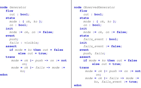
node Generator flow out : bool; state mode : { ok, ko }; on: bool; init

mode := ok, on := false; event

push;

fails : visible; assert

ifmode = ko then out = false else out = true;

trans

mode = ok |-push -> on:= not

on;

mode = ok |-fails -> mode :=

ko; edon node ObservedGenerator flow out : bool; state mode : { ok, ko }; on : bool; init

mode := ok, on := false; state fails_event : bool; init fails_event := false; event push, fails; assert

if mode = ko then out = false else out = true;

trans

mode = ok |- push -> on := not

on;

mode = ok |- fails ->mode :=

ko, fails_event := true; edon

Figure 2.1:An AltaRica node (left) and the observed version of the same node (right). One wants to observe occurrences of the failure event called fails_{. A new Boolean variable fails event is added to the model and} transitions labelled by fails now set to true the new variable.

C0 C1 a b C0, ha ← 0, b ← 0i C1, ha ← 1, b ← 0i C1, ha ← 0, b ← 1i a b

Figure 2.2: Even if configurations are reachable in both graphs, the state graph of the observed model is impacted by vectors that records occur-rences of events.

state then there exists a sub-sequence that can be repeated as many time as we want (i.e a loop). Clearly such sequences are irrelevant for risk assessment or diagnosis and algorithms should ignore them.

Our objective in this section is to design an algorithm similar to the one used to compute cuts. This latter consists to synchronize the model with an observer that records sufficient data to encode scenarios. Since AltaRica does not sup-port dynamic creation of variables, an upper bound to the state space required to store the current sequence must be known in advance. But, contrary to cuts, it is difficult to get this bound suitable to store the longest sequence (remember that events can be repeated). These considerations leads us to design the algo-rithm with the hypothesis that the length of sequences, the number of visible events, is fixed in advance by the user. Under this hypothesis it becomes feasi-ble to write an observer that requires only a ”small” amount of memory cells (i.e. variable) to encode sequences. Actually, the number of additional vari-ables should remain reasonable because, even if scenarios composed of more than five events are theoretically possible, they are, from a probabilistic point of view, extremely rare; thus users should look for sequence of length less or equal to 4 visible events.

2.4.1

Description of the algorithm

The algorithm proposed here is parameterized by the set of visible events EV and the maximal number k of visible events that can occur in a sequence. As already said, we follow the same principles than for algorithm used to compute cuts but this time we have to take into account the ordering of events and to translate the resulting DD into a set of sequences.

To record events and their logical order of appearance we can use at least two solutions reviewed in following subsections.

2.4.2

Memorizing when events occurs

First we can memorize when an event occurs. That means we have to store the logical instants when each visible event occurs. To realize this observer we use integer variables seen as vectors of bits. Each bit models a “visible” instant1_. This solution requires two operations:

• Firstly, we create a global integer variable tick that ranges in [1, 2k−1_{] used} to model the tick of visible events; k is the maximal length specified by the user. After each occurrence of a visible event the variable is multiplied by 2 i.e the bit encoding the instant is shifted by one position. tick is initialized to 1.

1_{This means that, using this implementation, sequences must be bounded by the number of bits} of a computer word (e.g. 32 or 64 bits).

• Then, for each visible event e ∈ EV we create an integer variable vethat takes its values into the range [0, 2k_{− 1] and is initialized with 0. To} re-member that e occurs at the current instant we add tick to the current value of ve. For instance if abac is a sequence of visible events then, reached configurations should be such that va= 20_{+ 2}2_{= 5, vb= 2}1_{= 2} and vc = 23_{= 8.}

Figure2.3describes a small system simply composed of two parallel com-ponents that may fail. Figure2.4gives the constraint automaton of this system decorated with variables as presented above. If for this system we want to obtain sequences that yield configurations such that c[0].s = nok within 3 visible events, then we get a DD that encodes the relation, given table2.1(page

18), over the three variables of the observer (the fourth column indicates the corresponding sequence – c[i] is used for c[i].failure):

node Component event action, repair; failure : visible; state s : { ok, nok }; init s := ok; trans s = ok |- failure -> s := nok; s = nok |- repair -> s := ok; s = ok |- action -> ; edon node Main sub c : Component[2]; edon

Figure 2.3: A simple model composed of two parallel components that may fail.

Memorizing what is the ith_event

The second method consists to memorize what happens at each instant. In other terms we have to remember the fact that the ith_{(visible) event was some} visible event e. To implement this solution the observer needs only k variables: • First we assign to each event e ∈ EV an integer id(e) in the range [1, N ]

where N = |EV| is the number of visible events.

• Then, we add k variables p1, . . . , pk, taking their values in the range [0, N ] and initialized with 0. Each pistores the event that occurs at the ith in-stant. pi is 0 if there is no ith_{event. Note that we have to ensure (see} below) that if piequals 0 then for all j > i, pjalso equals 0.

node DecoratedMain state ’c[0].s’ : { ok, nok }; ’c[1].s’ : { ok, nok }; tick : [1,4]; ’v c[0].failure’ : [0,7]; ’v c[1].failure’ : [0,7]; init ’c[1].s’ := ok, ’c[0].s’ := ok,

tick := 1, ’v c[0].failure’ := 0, ’v c[1].failure’ := 0; event

’c[0].failure’, ’c[1].failure’ : visible; ’c[0].repair’, ’c[1].repair’; trans (’c[1].s’ = nok) |- ’c[1].repair’ -> ’c[1].s’ := ok; (’c[1].s’ = ok) |- ’c[1].failure’ -> ’c[1].s’ := nok, tick := 2 * tick,

’v c[1].failure’ := ’v c[1].failure’ + tick; (’c[0].s’ = nok) |- ’c[0].repair’

-> ’c[0].s’ := ok;

(’c[0].s’ = ok) |- ’c[0].failure’ -> ’c[0].s’ := nok,

tick := 2 * tick,

’v c[0].failure’ := ’v c[0].failure’ + tick; edon

Figure 2.4: The constraint automaton is obtained by flattening the model given on figure 2.3; then it is decorated to observe up to k = 3 occurrences of events tagged with the visible attribute i.e EV = {c[0].failure, c[1].failure}. Additional data inserted to model the ob-server are underlined.

tick ’v c[0].failure’ ’v c[1].failure’ sequence 1 1 0 c[0] 2 1 2 c[0] c[1] 2 2 1 c[1] c[0] 2 3 0 c[0] c[0] 4 1 6 c[0] c[1] c[1] 4 2 5 c[1] c[0] c[1] 4 3 4 c[0] c[0] c[1] 4 4 3 c[1] c[1] c[0] 4 5 2 c[0] c[1] c[0] 4 6 1 c[1] c[0] c[0] 4 7 0 c[0] c[0] c[0]

Table 2.1: Sequences that yield c[0].s = nok. The first column gives the last value of tick variable. The next two columns give values of vari-ables that store occurrences of failures when the unexpected configuration is reached and the last column gives the corresponding sequence of fail-ures. Grey line for instance indicates that the sequence contains 3 events (tick = 23₋1

= 4). The failure of c[0] occurs at the second position because ’v c[0].failure’is equal to 2 i.e the bitvector 10. The failure of c[1] occurs at the first and third visible instant because ’v c[1].failure’ is equal to 5 i.e the bitvector 101.

– We extend the guard with the condition pk = 0. This means that after the kth_{visible event, all visible events are disabled}2_.

– We add assignments:

∗ p1:= if p1= 0 then id(e) else p1

∗ p2:= if p16= 0 ∧ p2= 0 then id(e) else p2 ∗ . . .

∗ pk := if p16= 0∧· · ·∧pk−16= 0∧pk = 0 then id(e) else pk which mean that each pireceives the event encoded by id(e) if and only if for all visible instant j < i, pj 6= 0 i.e visible events occur before instant i and no event has been recorded at instant i.

Figure2.5(page19) applies this method on the same system than for the previous example2.4. For this observer we obtain the relation, given table2.2

(page20), over pis variables (c[0].f ailure is assigned value 1 and c[1].f ailure the value 2).

2_{A similar disabling condition also exists for the first methods but it is implicit. Actually, since} tick_{is strictly increasing, it can not be assigned after the k}th_{visible event}

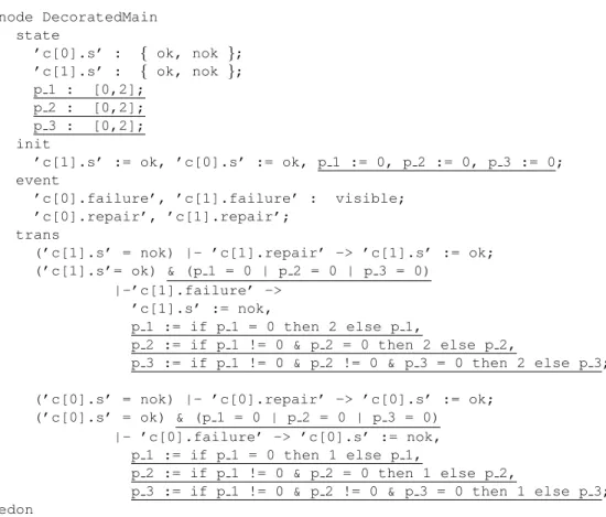
node DecoratedMain state ’c[0].s’ : { ok, nok }; ’c[1].s’ : { ok, nok }; p 1 : [0,2]; p 2 : [0,2]; p 3 : [0,2]; init ’c[1].s’ := ok, ’c[0].s’ := ok, p 1 := 0, p 2 := 0, p 3 := 0; event

’c[0].failure’, ’c[1].failure’ : visible; ’c[0].repair’, ’c[1].repair’;

trans

(’c[1].s’ = nok) |- ’c[1].repair’ -> ’c[1].s’ := ok; (’c[1].s’= ok) & (p 1 = 0 | p 2 = 0 | p 3 = 0)

|-’c[1].failure’ -> ’c[1].s’ := nok,

p 1 := if p 1 = 0 then 2 else p 1,

p 2 := if p 1 != 0 & p 2 = 0 then 2 else p 2,

p 3 := if p 1 != 0 & p 2 != 0 & p 3 = 0 then 2 else p 3; (’c[0].s’ = nok) |- ’c[0].repair’ -> ’c[0].s’ := ok;

(’c[0].s’ = ok) & (p 1 = 0 | p 2 = 0 | p 3 = 0) |- ’c[0].failure’ -> ’c[0].s’ := nok,

p 1 := if p 1 = 0 then 1 else p 1,

p 2 := if p 1 != 0 & p 2 = 0 then 1 else p 2,

p 3 := if p 1 != 0 & p 2 != 0 & p 3 = 0 then 1 else p 3; edon

Figure 2.5: Augmented constraint automaton for the same system and diagnosis objective than previously for example on figure2.3. This time, automaton is decorated using variables (pis) that memorize what happens at the ith

p 1 p 2 p 3 sequence 1 0 0 c[0] 1 1 0 c[0] c[0] 1 2 0 c[0] c[1] 2 1 0 c[1] c[0] 1 1 1 c[0] c[0] c[0] 1 1 2 c[0] c[0] c[1] 1 2 1 c[0] c[1] c[0] 1 2 2 c[0] c[1] c[1] 2 1 1 c[1] c[0] c[0] 2 1 2 c[1] c[0] c[1] 2 2 1 c[1] c[1] c[0]

Table 2.2: Sequences that yield c[0].s = nok computed using the sec-ond encoding. The first three columns give values of pivariables i.e. which visible event has occurred at the ith

position. Last column gives the cor-responding sequence. Value 0 means no event occurs, 1 means failure of c[0] and 2 means failure of c[1]. Grey line for instance indicates that the sequence contains 2 events because the last non-zero pivariable is p2. The first event is the failure of c[1] (value is 2) and the second event is the failure of c[0] (value is 1).

Comparison of methods

Both methods have to be used within reachability analysis based on decision diagrams. Even if observer partially reduces behaviours of the system (oc-currences of failures are stopped after the kth _{one), the introduction of new} variables should not reduce the size of computed relations, especially for in-termediate ones that are known to be larger than the final relation (the one encoding reachable configurations).

Clearly the first method has the drawback to generate lots of variables. If we consider the largest model treated during our experiments (cf. chapter chapter6), reduced automata can have around 20 and 80 events. The second method produces only k variables but each variable takes as many values as there exists visible events and thus the size of computed relations is unpre-dictable. However decision diagrams implemented inARCuse a compact en-coding of ranges that should help to keep the size of relations manageable.

Although the second method seems to be the best one it has a second minor drawback. Up to now, we have considered events of the flattened constraint automaton; that means the observer memorizes vectors of events and not ele-mentary events (those specified in nodes). It happens that for models (see6), elementary events are not explicitly synchronized so there is a one-to-one cor-respondence between elementary and global events. The first method is able to handle both kind of events; it suffices to create a variable for each elemen-tary event and to assign in transitions each elemenelemen-tary events appearing in the

labelling vector. The second method can handle only global events. It could be adapted by duplicating pis variables as many time as there is events in the largest vector but the method would become too costly. In fact the handling of vectors can be postponed, if actually necessary, to the end of the computation process.

2.5

Implementation

ARC implements the algorithm that computes cuts and the second algorithm (section2.4.2) for sequences. The principle of these implementations is quite simple; it is based on the symbolic computation of reachable configurations already implemented inARC. We illustrate this algorithm on figure2.6.

1. After the computation of the flat semantics[13], variables of the observer are added to the constraint automaton equivalent to the original model. 2. ARCsymbolically computes the set of reachable configurations of the

ob-served model A × Obs. This set is represented by a Decision Diagram (DD)[5]. This DD is represented in grey on the figure. For the sake of clarity we have assumed that variables of the observer are at the bottom of the diagram but in practice all variables are mixed.

3. Then, the set of reachable configuration is intersected with those that sat-isfy φ. This gives us a new DD depicted in red and green.

4. This second DD is then projected on the observer part i.e., event variables ve’s for cuts or pis variables for sequences. This is the green DD of the figure.

5. This last DD contains all data necessary to produce cuts or sequences; it suffices to translate it into the appropriate format to get the result: either Boolean formulas or list of sequences.

Obs A

Remark about sequences: ARC produces sequences using the second algo-rithm (section2.4.2). Generated scenarios are lists of global events. The mini-mization algorithm (see chapters3and4) is applied on such sequences which means that:

• it can produce sequences like (ha, b, ci, a) where two global events having common elementary events appear (here the vector ha, b, ci and a alone). • if (ha, b, ci) and (a) are two generated sequences (i.e that produces the diagnosis objective), the former is not removed by the minimization al-gorithm that consider both events as unrelated.

Chapter 3

Residual Language Decision

Diagrams

In this chapter we present a data structure defined in [13] similar to Zero-suppressed BDDs (ZBDD) introduced by S. Minato[12]. While ZBDDs permit to store finite sets of subsets, RLDDs encode finite sets of words. This data structure allows classical operations over sets like union or intersection but also a minimization operation that computes minimal sequences (for the sub-word order). Recently this data structure has been studied in the context of data-mining under the name of SeqBDD [7,11].

3.1

Residual languages and RLDDs

In the sequel we consider a finite alphabet Σ. A word w is a sequence a1a2. . . an of letters ai belonging to Σ. The number of letters in a word is its length; we denote by ǫ the word of length 0. The set of words over Σ built with n letters is denoted Σn_{. The set of all words (ǫ included) over Σ is denoted Σ}⋆_{. A language} over Σ is any subset of Σ⋆_.

The concatenation of two words w1, w2 taken in Σ⋆ _{is denoted w1.w2; ǫ is} the identity element for concatenation. If w ∈ Σ⋆ _{is a word and L ⊆ Σ}⋆ _a language then w.L is the language {w.x | x ∈ L} i.e., the set of words formed by w followed by any word belonging to L.

For any language L ⊆ Σ⋆_{and any letter a ∈ Σ, the residual language of L by} a is the language denoted by a−1_{L and defined by:}

a−1L = {u ∈ Σ⋆| a.u ∈ L}

The reader should notice that a−1L is not necessarily a subset of L and, as shown on following example, a.(a−1L) is not always L but the set of residual languages of L is a partition of L: L = ∪a∈Σa.(a−1_L).

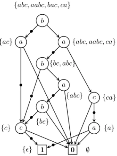
Example 2 Let Σ = {a, b, c, d} and L = {abc, aabc, bac, ca}. Then: a−1L = {bc, abc}, b−1_{L = {ac}, c}−1_{L = {a}, d}−1_{L = ∅.}

In the sequel we will use the following notations:

• La = a.(a−1L) the subset of L whose words start with letter a. • La = L \ Lathe words of L that do not start with a.

Laand Lais a partition of L i.e La∩La = ∅ and La∪La= L. This decompo-sition of L is used to defined a data structure to store any finite language L in a compact way. The previous partitioning plays the same role as the well-known Shannon decomposition theorem used to build BDDs[2].

We have called this data structure RLDD for Residual Language Decision Diagram. As other decision diagrams, a RLDD is a directed acyclic graph (DAG).

Definition 2 (RLDD) A RLDD is a DAG with three kind of nodes: • either one of the two leaves 0 or 1

• or an intermediate node denoted N = ha, N1, N2i where a ∈ Σ is the label of the node and, N1and N2are children nodes of N .

Definition 3 (Height) The height H(N ) of a RLDD N is defined inductively by: • H(0) = H(1) = 0

• H(ha, N1, N2i) = 1 + max(H(N1), H(N2))

Definition 4 (Semantics) The semantics of a RLDD N is a language denoted JN K ⊆ Σ⋆_{defined recursively on the structure of RLDDs:}

• J0K = ∅ • J1K = {ǫ}

• Jha, N1, N2iK = a.JN1K ∪ JN2K

A RLDD encoding the language L given in example2 is depicted on fig-ure3.1. When represented graphically, the edge between an intermediate node and its left child is decorated with a black bullet • (to recall concatenation op-eration).

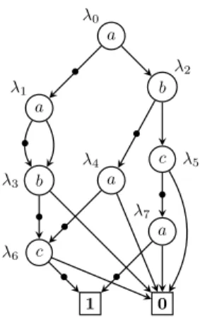
Depending on letters used to decompose successive residuals the RLDD encoding a language L is different. For instance the figure3.2depicts a RLDD encoding the same language than the one on figure3.1. While on the first figure (3.1) letters were always selected in the order b, a and c, on the second one, letters were chosen in the order a, b and c.

To ensure canonicity of the representation and to improve efficiency of al-gorithms we have to enforce the choice of the letter used to decompose a lan-guage. In the sequel we assume that Σ is an alphabet completely ordered by

1 {ǫ} 0 _∅ c {c} a {a} c {ca} b {bc} a {abc} b {bc, abc}

a {abc, aabc, ca} b

{abc, aabc, bac, ca}

a {ac} • • • • • • • • •

Figure 3.1:A RLDD encoding L = {abc, aabc, bac, ca}.

some relation <. The letter ρ(L) used to decompose a language L is defined according to this order as the smallest letter that gives a non-empty residual language:

Definition 5 (Decomposition letter) For any non-empty language L that is not the singleton {ǫ}, we define:

ρ(L) = min<({a ∈ Σ | a−1L 6= ∅})

For any finite language L ⊆ Σ⋆_{, the canonical RLDD representing L, RLDD(L)} is defined by:

• RLDD(L) = 0 if L is empty; • RLDD(L) = 1 if L is {ǫ};

• RLDD(L) = ha, RLDD(a−1_{L), RLDD(La)i where a = ρ(L).}

Example 3 We come back on the language given in example2. Now we consider that Σ is ordered as follows: a < b < c. The canonical RLDD encoding L is given on the figure3.2. This RLDD has been built as follows:

• λ0 = RLDD({abc, aabc, bac, ca}) = ha, RLDD({bc, abc}), RLDD({bac, ca})i = ha, λ1, λ2i

• λ1= RLDD({bc, abc}) = ha, RLDD({bc}), RLDD({bc})i = ha, λ3, λ3i • λ2= RLDD({bac, ca}) = hb, RLDD({ac}), RLDD({ca})i = hb, λ4, λ5i • λ3= RLDD({bc}) = hb, RLDD({c}), ∅i = hb, λ6, 0i

1 0 c λ6 a λ7 c λ5 b λ3 a λ4 a λ1 b λ2 a λ0 • • • • • • • •

Figure 3.2: RLDD encoding the same language that the RLDD on figure

3.1. The order a < b < c is used.

• λ5= RLDD({ca}) = hc, RLDD({c}), ∅i = hc, λ7, 0i • λ6= RLDD({c}) = hc, RLDD({ǫ}), ∅i = hc, 1, 0i • λ7= RLDD({a}) = ha, RLDD({ǫ}), ∅i = ha, 1, 0i

3.2

Basic operations on RLDDs

In this section we present three basic operations that are required to compute minimal words. These operations, build, union and intersection, are defined recursively on the structure of their operands. In the sequel, if N = ha, N1, N2i is a RLDD we denote:

• λ(N ) its label a; • α(N ) its left child N1; • and β(N ) its right child N2.

The build operator is used to ensure that left child is not empty.

Build: build_{: Σ × RLDD × RLDD −→ RLDD} • build(a, 0, Y ) = Y for any RLDD Y ;

Union union_{: RLDD × RLDD −→ RLDD} • union(X, X) = X for any RLDD X

• union(0, X) = union(X, 0) = X for any RLDD X

• union(1, N ) = union(N, 1) = hλ(N ), α(N ), union(1, β(N ))i • union(N1, N2) = ha, N, N′_{i where:}

– a = min(λ(N1), λ(N2))

– if λ(N1) = λ(N2) then N = union(α(N1), α(N2)) and N′_{= union(β(N1), β(N2))}

– if λ(N1) < λ(N2) then N = α(N1) and N′_{= union(β(N1), N2)}

– if λ(N1) > λ(N2) then N = α(N2) and N′_{= union(N1, β(N2))}

Intersection inter_{: RLDD × RLDD −→ RLDD} • inter(X, X) = X for any RLDD X

• inter(0, X) = inter(X, 0) = 0 for any RLDD X • inter(1, N ) = inter(N, 1) = inter(1, β(N )) • inter(N1, N2) = N where:

– if λ(N1) = λ(N2) then N = build(λ(N1), inter(α(N1), α(N2)), inter(β(N1), β(N2)))

– if λ(N1) < λ(N2) then N = inter(β(N1), N2)

– if λ(N1) > λ(N2) then N = inter(N1, β(N2))

Theorem 1 For any letter a ∈ Σ and any RLDDs X and Y , • Jbuild(a, X, Y )K = a.JXK ∪ JY K

• Junion(X, Y )K = JXK ∪ JY K • Jinter(X, Y )K = JXK ∩ JY K

Proof: By induction on H(X) + H(Y ). ♦

3.3

Minimal words

Given a set of words seen as critical scenarios, several criteria can be imagined to determine which words are the most representatives. In the sequel we will denote by u ⊑ v the fact that u is more important than v.

The simplest criterion is certainly the length of words but it is too strong. Of course it selects shortest scenarios so the most important ones, but it com-pletely ignores qualitative informations of sequences. For instance, if a and

bc are two failure sequences that involve separate parts of the system, bc is rejected.

A second criterion could be the prefix order. We consider that a sequence u ⊑ v if u starts (or is a prefix of) v. This criterion mixes length and qualitative informations. Actually if u is a prefix of v, u is more probable than v and taking countermeasures to prevent u should resolve issues for v. However, the crite-rion is too weak because it keeps useless sequences. For instance, abc and bc can not be compared with the prefix order; so both are kept while, clearly, abc should be forgotten. In this case, a comparison of suffixes should be preferred. The factors can also be used. u ⊑ v if v = x.u.y where x and y are arbitrary and possibly empty words; u is said to be a factor of v. This criterion gathers advantages of length, prefixes, suffixes and handles what happens in the “mid-dle” of sequences. But factors ignore the case where letters of u are dispatched into v i.e. for instance abc and ac.

Finally a fourth criterion will be used and, intuitively it is very similar to the one used for cuts (i.e. inclusion). For now on, we consider that u ⊑ v if u is a sub-word of v. More formally, we define this order as follows.

Definition 6 (Subwords) Let u = u1. . . un and v = v1. . . vm be two words of

length n and m respectively. u is a sub-word of v if there exists a mapping σ : [1, n] → [1, m] such that:

1. σ is strictly increasing i.e. for any 1 ≤ i < j ≤ n, σ(i) < σ(j); 2. ∀i ∈ [1, n], ui= vσ(i)

The above definition simply describes the fact that if u is a subword of v (u ⊑ v) then letters of u can be dispatched into v with respect of their order in u.

3.3.1

A decomposition theorem for sub-words

The computation of minimal words of L is based on a simple idea: 1. First, L is split into two disjoint subsets, say X and Y ;

2. Then, we remove from X words that have a sub-word in Y and con-versely, we remove from Y words that have a sub-word in X.

3. Finally, we join together obtained sets to get minimal words min⊑(L). For the first step, a partition of language L is obtained easily using residual languages. If a = ρ(L) then we choose to split L as La and La. The second step requires the introduction of a new operation over languages; we denote this operation ÷ (as in [16]). This operation removes from a language X all words that are not minimal with respect to words of a second language Y . More formally, ÷ is defined by:

This operation ÷ has the following properties for all subsets X, Y and Z of Σ⋆_{and letters a, b ∈ Σ:} 1. X ÷ ∅ = X 2. X ÷ {ǫ} = ∅ 3. (X ∪ Y ) ÷ Z = X ÷ Z ∪ Y ÷ Z 4. X ÷ (Y ∪ Z) = X ÷ Y ∩ X ÷ Z 5. a.X ÷ a.Y = a.(X ÷ Y )

6. a 6= b ⇒ a.X ÷ b.Y = a.(X ÷ b.Y )

7. X ÷ Y = [(Xa÷ Ya) ∩ (Xa÷ Ya)] ∪ (Xa÷ Y )

Lemma 1 ∀L ⊆ Σ⋆_{\{ǫ}, ∀a ∈ Σ, ∀w ∈ Σ}⋆_{, a.w ∈ min(L) ⇐⇒ w ∈ min(a}−1_L)÷ La

Proof: Assume that a.w ∈ min(L). We have w ∈ a−1L. There is no v ∈ a−1_L such that v ⊏ w because we would have a.v ⊏ a.w which refutes a.w ∈ min(L); thus, w ∈ min(a−1_{L). If v ∈ Lais such that v ⊏ w yields the same contradiction} because, in this case, v ⊏ a.w.

For the converse, let w ∈ min(a−1_{L) ÷ La and v ∈ L such that v ⊑ a.w.} If v = a.x with x ∈ Σ⋆_{, we have x ⊏ w which contradicts w ∈ min(a}−1_{L). If} v ∈ La i.e v = b.x with x ∈ Σ⋆_{, we have b.x ⊏ w but it is impossible because w}

would have been removed from min(a−1_{L) by ÷. ♦}

Lemma 2 ∀L ⊆ Σ⋆_{\ {ǫ}, ∀a, b ∈ Σ, ∀w ∈ Σ}⋆_{, a 6= b ⇒ (b.w ∈ min(L) ⇐⇒} b.w ∈ min(La) ÷ La)

Proof: Let b.w ∈ min(L); clearly b.w ∈ min(La). The hypothesis imposes that for any a.x ∈ La, a.x 6⊏ b.w; so b.w ∈ min(La) ÷ La. For the converse, assume b.w ∈ min(La) ÷ La and x ∈ L such that x ⊏ b.w. x can not be in La because b.w would have been removed from min(La) by ÷. x can neither be in Labecause b.w ∈ min(La). We can conclude that for x ∈ L, x 6⊏ b.w and, thus,

b.w ∈ min(L). ♦

Corollary 1 (Decomposition of sets of minimal words)

∀L ⊆ Σ⋆_{, ∀a ∈ Σ, min(L) = a.(min(a}−1_{L) ÷ La) ∪ (min(La) ÷ La)} The previous theorem shows that computation of minimal words can fol-lows the structure of languages given by their residual languages. This result permits us to easily design an algorithm computing min⊑based on the RLDD data structure.

3.3.2

Application to RLDDs

In order to compute minimal sequences we have to define ÷ and min for RLDDs. As others, these operations, called respectively div and minimize, are defined according to the RLDD structure:

Extraction div_{: RLDD × RLDD −→ RLDD} • div(0, X) = 0 for any RLDD X

• div(X, 0) = X for any RLDD X • div(X, 1) = 0 for any RLDD X • div(1, N ) = div(1, β(N ))

• div(N, N′_{) = build(λ(N ), N1, N2) where:}

– if λ(N ) = λ(N′_{), N1= inter(div(α(N ), α(N}′_{)), div(α(N ), β(N}′_))),

– if λ(N ) 6= λ(N′_{), N1= div(α(N ), N}′₎

– N2= div(β(N ), N′)

Theorem 2 For any RLDDs N , Jdiv(N, N′_{)K = JN K ÷ JN}′_K

Proof: We show the result by induction on n = H(N ) + H(N′). We consider only the last case. We assume the property satisfied for any k < n. Let N and N′_{, two RLDDs such that H(N ) + H(N}′_{) = n. Let a = λ(N ) and a}′ _{= λ(N}′_). We consider the two cases;

a_{= a}′_{: By construction we have:}

Jdiv(N, N′)K = a.(Jdiv(α(N ), α(N′))K∩Jdiv(α(N ), β(N′))K)∪Jdiv(β(N ), N′)K Then, induction hypothesis gives us:

Jdiv(N, N′_{)K = a.(Jα(N )K ÷ Jα(N}′_{)K ∩ Jα(N )K ÷ Jβ(N}′_{)K) ∪ (Jβ(N )K ÷ JN}′_K) = a.(Jα(N )K ÷ Jα(N′_{)K) ∩ a.(Jα(N )K ÷ Jβ(N}′_{)K) ∪ (Jβ(N )K ÷ JN}′_K) Using properties5and6of ÷ we get:

Jdiv(N, N′_{)K = (a.Jα(N )K ÷ a.Jα(N}′_{)K) ∩ (a.Jα(N )K ÷ Jβ(N}′_{)K) ∪ (Jβ(N )K ÷ JN}′_K) = (a.Jα(N )K ÷ (a.Jα(N′_{)K ∪ Jβ(N}′_{)K)) ∪ (Jβ(N )K ÷ JN}′_K)

= (a.Jα(N )K ÷ JN′_{K) ∪ (Jβ(N )K ÷ JN}′_K) = (a.Jα(N )K ∪ Jβ(N )K) ÷ JN′K

a_{6= a}′_{: We use the same method but this time we have:}

Jdiv(N, N′_{)K = a.(Jdiv(α(N ), N}′_{)K) ∪ Jdiv(β(N ), N}′_)K Then, induction hypothesis gives us:

Jdiv(N, N′)K = a.(Jα(N )K ÷ JN′K) ∪ (Jβ(N )K ÷ JN′K) = (a.Jα(N )K ÷ JN′_{K) ∪ (Jβ(N )K ÷ JN}′_K) = (a.Jα(N )K ∪ Jβ(N )K) ÷ JN′_K) = JN K ÷ JN′_K ♦ Minimization minimize_{: RLDD −→ RLDD} • minimize(0) = 0 • minimize(1) = 1

• minimize(N ) = build(λ(N ), N1, N2) where:

– N1= div(minimize(α(N )), β(N ))

– N2= div(minimize(β(N )), build(λ(N ), α(N ), 0))

Theorem 3 For any RLDD N , Jminimize(N )K = min(JN K)

Proof: Straightforwards by induction on the structure of RLDDs. ♦

3.4

Complexity

In above section, algorithms are specified using recursive equations based on the structure of RLDDs. Applying these algorithms as-is could yield execution times exponential into the height of diagrams. This exponential cost comes from multiple recursive calls that visit several times a same path. The well-known technique of computation caches (e.g. [3]) must be used to reduced the number of redundant visits of paths.

Unfortunately div operation can yield diagrams with an exponential num-ber of nodes while its arguments have a polynomial size. This cost can not be absorbed by cache techniques. For instance, if Σ is an alphabet with n letters, then

Un = {u ∈ Σn _{| ∀a ∈ Σ, |u|a= 1}}

where |u|ais the number of letters a in u, is a language that requires n2n−1_{+ 2} nodes to be represented by a RLDD. Un is the set of words composed of n distinct letters. Un can be obtained by applying ÷ to two languages that are encoded with a polynomial number of nodes:

1. Σn_{the set of words of length n that requires n}2_{+ 2 nodes;}

2. Sqr(Σ) = {a.a | a ∈ Σ} the set of words of length 2 containing twice the same letter. This language requires 2n + 2 nodes.

We have Un = Σn _{÷ Sqr(Σ) because Sqr(Σ) removes from Σ}n _{words with} multiple occurrences of same letters. Figures3.3,3.4and3.5depict respectively Σn_{, Sqr(Σ) and Unfor an alphabet Σ containing 3 letters.}

The size of Un in terms of RLDD nodes, n2n−1_{+ 2, has been obtained} ex-perimentally but it can be proved that the same phenomenon also holds for minimal automata that recognize Σn_{, Sqr(Σ) and Unwhich have, respectively,} n + 1, n + 2 and 2n_states1_.

In practice, in the context of failure scenarios computation, such diagrams should not be problematic because languages (i.e. sets of scenarios) would con-tain few (around one hundred words) and short words (less than ten events).

1 0 c b a c b a c b a • • • • • • • • • Figure 3.3: A RLDD encoding {a, b, c}3 1 0 c b a c b a • • • • • • Figure 3.4: A RLDD for Sqr({a, b, c}). a b c a b a b a c c c b 1 0 • _• • • • • • • _• • • •

Figure 3.5:A RLDD encoding U3= {a, b, c} 3

Chapter 4

Minimal cuts and minimal

sequences

This chapter presents algorithms used to minimize sets of sequences and sets of cuts computed using algorithms presented in chapter2.

Both algorithms (for sequences and cuts) take as input a Decision Diagram[5] representing all computed scenarios that yield an unexpected configuration. Minimization algorithms are based on RLDDs (see chapter3). However, since the encoding of scenarios by means of DDs is not the same in both cases, we have to write two specific translation algorithms.

4.1

A brief introduction to DDs

Decision Diagrams (DD) used byARC[9] model-checker, are stemmed from the

TOUPIEtool[5]. DDs are diagrams built over non-Boolean variables. Domains

of variables remain finite but they can contain an arbitrary number of elements. The principle is the same than for BDDs but, instead of taking the decision according to two values we use N values (if N is the cardinality of the domain of the variable).

DDs are used inARCto represent sets of configurations, relation transitions or more generally relations. Figure4.1gives an example of a DD that represents reachable configuration of an AltaRica node.

In the context of scenarios generation, variables are added to AltaRica nodes to record occurrences of events. After the computation of reachable configura-tions, the DD is projected on these additional variables (i.e. all other variables are removed) to keep only data related to expected scenarios. Depending on the nature of computed objects, sets or words, resulting DDs have different se-mantics and different structures. Figure4.2depicts DDs that encode the same scenarios abc, ac and b but in a one case they are viewed as cuts and in the other case, as sequences.

node A flow i, o : [0, 2]; state s : { ok, nok }; event fail; trans s = ok |- fail -> s := nok; assert

o = (if s = ok then i else 0); edon s i o o o i 1 0 0 1 0 1 2 0 1 0 1..2 1 0 2 0..1 2

Figure 4.1:An AltaRica node and the DD encoding its reachable configu-rations. Symbolic values ok and nok are encoded by integer values 0 and 1.

4.2

Sequence and minimal sequences

As mentioned in introduction, minimization algorithm is based on RLDDs. We could design a direct computation of minimal sequences from the DD that encodes sequences but we have preferred to generate an intermediate structure that permits to easily manipulate and display the whole set of sequences.

The main issue is thus to translate the DD that encodes computed sequences into a RLDD and then to apply the minimization operator defined over RLDDs (see3.3). This translation step is straightforward if pis variables that memorize ith_{events are ordered according to i in the DD. If this is not the case a simple} relabelling of variables is realized. Under the hypothesis of a good ordering of variables, algorithm2(page37) translates a DD into a RLDD. In the pseudo-code of algorithm2 we have use suffixes DD and RL to distinguish trivial nodes (0 and 1) of DDs and RLDDs.

Due to the encoding of sequences by pi variables, the DD can be viewed as a classical automaton recognizing words where 1DDis the accepting state,

0DD is a sink state and 0-labelled edges are interpreted as ǫ transitions. The algorithm recursively visits paths to the accepting state (i.e the leaf node 1DD) using a depth-first search traversal of the input DD.

As usual a cache C is used (lines7and17) to prevent useless revisit of same paths of the DD; if the cache does not erase its entries the number of recursive calls is linear in the number of nodes of the DD.

Figure4.3shows the application of algorithm2on the DD depicted on the right side of figure4.2. Note that, on this example the cache is useless; except leaves, all DD nodes have only one input edge.

b

{{b, a, c}, {b, a, c}, {b, a, c}}

a

{{a, c}} a {{a, c}, {a, c}}

c {{c}} c {{c}} 1 {∅} 0 _∅ 0 1 1 0 1 0 1 0 1 0 p1 {abc, ac, b} p2 {bc, c} p2 {ǫ} p3 {c} {ǫ} p3 p3 {ǫ} 1 {ǫ} 0 _∅ 1 (a) 2 (b) 2 (b) 3 (c) 0 3 (c) 0 0 0,3 0,1 1..3 0..2 1..3 1..3

Figure 4.2: Different representations of scenarios abc, ac and b by means of DDs. On the left hand side, scenarios are considered as cuts (note that in this case, b and ac are implicit in ac and b). Each variable of the DD corresponds to an event and are ordered as b < a < c. Edges to leaf node 0 are drawn in gray. On the right hand side, scenarios are viewed as sequences where a = 1, b = 2 and c = 3 (recall observer described in chapter2). Length of sequences is bound by k = 3. Note that for sequences with less than k events, scenarios are padded with 0s.

4.3

Minimal cuts

The algorithm is inspired by the one proposed by A. Rauzy in [16]. The origi-nal algorithm (section C of [16]) computes for a Boolean formula F a ZBDD[12] that encodes minimal cuts of F according to a set L of significant literals. Lit-erals can be positive and/or negative occurrences of elementary events. That means that non-failures could be considered as relevant informations.

In the context of this study we have chosen to ignore these negative infor-mations and to handle only positive events (i.e actual failures). This hypoth-esis corresponds to case 2 of Rauzy’s algorithm where, for all failure event e, e ∈ L and e 6∈ L. Algorithm3 is an implementation of Rauzy’s algorithm (case 2) using RLDDs instead of ZBDDs. Remember that DDs that encode cuts have at most two children nodes because the observer uses only Boolean vari-ables. The function variable(N ) returns the index of the variable labelling the node. cofactor(N, i) returns the ith_{child of N .}

Figure4.4depicts application of algorithm3on the DD depicted on the left side of figure4.2.

The main difference between Rauzy’s algorithm and algorithm3is the use of rldd-div instead of the similar operation ÷ defined in [8] for ZBDDs. This replacement can be easily justified by the fact that due to ordering of variables, cuts are implicitly treated as words. More precisely, if for any cut σ, we denote by w(σ) the word obtained by concatenating elements of σ according to the

Algorithm 2dd-to-rldd(DD N , cache C) 1: RLDD R/* the result */ 2: if N = 0DDthen 3: R = 0RL 4: else if N = 1DDthen 5: R = 1RL 6: else 7: R = cache-find-operation(C, dd-to-rldd, N ) 8: if R = NULL then 9: R = 0RL

10: for alloutgoing edge N −→ Na ′_do

11: RLDD son = dd-to-rldd(N′, C)

/* a = 0 means that current pi was not assigned i.e the edge is treated as an ǫ. */

12: if a 6= 0 then

13: son = rldd-build(a, son, 0RL)

14: end if 15: R = rldd-union(R, son) 16: end for 17: cache-memorize-operation(C, dd-to-rldd, N, R) 18: end if 19: end if 20: return R

order used to build DDs, then for any cuts σ1 and σ2, σ1 ⊆ σ2 if and only if w(σ1) is a sub-word of w(σ2).

p1 {abc, ac, b} p2 {bc, c} p2 {ǫ} p3 {c} {ǫ} p3 {ǫ} p3 1 {ǫ} 0 ∅ 1 2 2 3 0 3 0 0 0,3 0,1 1..3 0..2 1..3 1..3 1 {abc, ac, b} 2 {bc, c} 2 {b} 3 {c} 1 {ǫ} 0 ∅ • • • •

Figure 4.3: Application of the dd-to-rldd algorithm onto the DD en-coding sequences abc, ac and b depicted on figure4.2. Dashed arrows show the mapping realized by the algorithm between DD (on the left) and RLDD nodes (on the right). Remember that letters a, b and c are encoded respectively by integers 1, 2 and 3. On DDs, letters label edges while on RLDDs, letters label nodes.

Algorithm 3dd-to-min-rldd(DD N , cache C)

1: RLDD R/* the result */ 2: if N = 0DDthen 3: R = 0RL 4: else if N = 1DDthen 5: R = 1RL 6: else 7: R = cache-find-operation(C, dd-to-min-rldd, N ) 8: if R = NULL then 9: int v = variable(N ) 10: DD N0= cofactor(N, 0) 11: DD N1= cofactor(N, 1) 12: RLDD son0 = dd-to-min-rldd(N0, C) 13: RLDD son1 = dd-to-min-rldd(N1, C) 14: RLDD tmp = rldd-div(son1, son0) 15: R = rldd-build(v, tmp, son0) 16: cache-memorize-operation(C, dd-to-min-rldd, N, R) 17: end if 18: end if 19: return R

b

{{b, a, c}, {b, a, c}, {b, a, c}}

a

{{a, c}} a {{a, c}, {a, c}}

c {{c}} c {{c}} 1 {∅} 0 ∅ 0 1 1 01 0 1 0 1 0 b {b, ac} a {ac} c {c} 1 {ǫ} 0 ∅ • • •

Figure 4.4:Application of the dd-to-min-rldd algorithm onto the DD encoding cuts abc, ac and b depicted on figure4.2. Dashed arrows show the mapping realized by the algorithm between DD (on the left) and RLDD nodes (on the right). Variables are ordered as follows: b < a < c.

Chapter 5

Reduction of models

5.1

Principles of the reduction

The reduction algorithm is applied to the constraint automaton[14] that repre-sents the model. This automaton, actually an AltaRica node, is obtained using a rewriting process that removes all hierarchical levels of the model and com-piles this latter into an equivalent n ode. This process has been called the flat semantics of the model[13].

Given a constraint automaton A that represents the system we want to eval-uate a Boolean formula φ built over variables of A. φ will be called target for-mula. Our goal is to reduce A to its only parts (i.e variables, assertions and transitions) that are mandatory to evaluate φ all along runs (or behaviours) of the automaton.

More precisely the restricted automaton, denoted Aφ_{, should satisfy} follow-ing properties:

1. For any configuration σ of A one can associate its projection σ′in Aφand σ satisfies φ iff σ′_{satisfies φ.}

2. For all executable sequences of macro-transitions of A, its restriction to macro-transitions belonging to Aφ_{is actually an executable sequence in} Aφ_.

3. Any executable sequence of macro-transitions of Aφ _{is an executable} se-quence of A.

The main idea that underlies the algorithm is to compute items that may influence the truth value of φ. Starting from variables appearing in φ, one com-putes elements of A related to these variables: flow variables are influenced by assertions, assertions by flow and state variables, state variables by transitions and so on. These relations between components of A permit to restrict A to a subset of its variables; other parts not related to these variables are simply ignored.