HAL Id: insu-01808646
https://hal-insu.archives-ouvertes.fr/insu-01808646
Submitted on 11 Jul 2018
HAL is a multi-disciplinary open access
archive for the deposit and dissemination of
sci-entific research documents, whether they are
pub-lished or not. The documents may come from
teaching and research institutions in France or
abroad, or from public or private research centers.
L’archive ouverte pluridisciplinaire HAL, est
destinée au dépôt et à la diffusion de documents
scientifiques de niveau recherche, publiés ou non,
émanant des établissements d’enseignement et de
recherche français ou étrangers, des laboratoires
publics ou privés.
Effects of the Crustal Magnetic Fields and Changes in
the IMF Orientation on the Magnetosphere of Mars:
MAVEN Observations and LatHyS Results.
Norberto Romanelli, Ronan Modolo, François Leblanc, Jean-Yves Chaufray,
Sébastien Hess, David Brain, Jack Connerney, Jasper Halekas, James
Mcfadden, Bruce Jakosky
To cite this version:
Norberto Romanelli, Ronan Modolo, François Leblanc, Jean-Yves Chaufray, Sébastien Hess, et al..
Effects of the Crustal Magnetic Fields and Changes in the IMF Orientation on the Magnetosphere of
Mars: MAVEN Observations and LatHyS Results.. Journal of Geophysical Research Space Physics,
American Geophysical Union/Wiley, 2018, 123 (7), pp.5315-5333. �10.1029/2017JA025155�.
�insu-01808646�
Effects of the Crustal Magnetic Fields and Changes in the IMF
Orientation on the Magnetosphere of Mars: MAVEN
Observations and LatHyS Results
N. Romanelli1 , R. Modolo1 , F. Leblanc2 , J-Y. Chaufray1 , S. Hess3 , D. Brain4 ,
J. Connerney5 , J. Halekas6 , J. Mcfadden7, and B. Jakosky4
1Laboratoire Atmosphere, Milieux et Observations Spatiales (LATMOS), IPSL, CNRS, UVSQ, UPMC, Paris, France, 2LATMOS/IPSL, UPMC, Univ Paris06 Sorbonne Universités, UVSQ, CNRS, Paris, France,3Office National d’Etudes et de
Recherches Aérospatiales, Toulouse, France,4Laboratory for Atmospheric and Space Physics, University of Colorado
Boulder, Boulder, CO, USA,5NASA Goddard Space Flight Center, Greenbelt, MD, USA,6Department of Physics and
Astronomy, University of Iowa, Iowa City, IA, USA,7Space Sciences Laboratory, University of California, Berkeley, CA, USA
Abstract
The Mars Atmosphere and Volatile EvolutioN Mission (MAVEN) is currently probing the complex Martian environment. Although main structures arising from the interaction between the solar wind (SW) and the induced magnetosphere of Mars can be described using a steady state picture, time-dependent physical processes modify the response of this obstacle. These processes result from temporal variabilities in the internal and/or external electromagnetic fields and plasma properties. Indeed, the crustal magnetic fields (CF) rotation constantly modifies the intrinsic magnetic field topology relative to the SW. Moreover, the magnetosphere’s state is also modified by changes in the interplanetary magnetic field (IMF). In this work we analyze MAVEN magnetic field and plasma measurements obtained on 23 December 2014, between 06:00 UT and 14:15 UT. These measurements suggest that the external conditions remained approximately constant when MAVEN was inside the magnetosphere during the first orbit. In contrast, MAVEN observed changes in the IMF orientation before visiting the magnetosphere during the second orbit. To investigate the response of the Martian plasma environment to the CF rotation and IMF variability, we also perform hybrid simulations, using MAVEN observations to set SW external conditions. Simulation results are compared with the MAVEN measurements and show good agreement. Associated recovery timescales of different magnetospheric regions are found to range between ∼ 10 s and ∼ 10 min. Finally, we do not observe large variability in the total planetary H+and O+escape rates atdifferent times during this event, although a correlation between the latter and the CF location is identified.
1. Introduction
Mars does not have a significant intrinsic global magnetic field (Acuña et al., 1998). As a result, there is a direct interaction between the magnetized solar wind (SW) and the atmosphere of this planet. As part of this inter-action, the atmosphere of Mars is subject to several ionizing mechanisms such as photoionization, charge exchange, and electron impact. Also, through several current systems (e.g., Baumjohann et al., 2010), it gen-erates perturbations in the streaming interplanetary magnetic field (IMF), leading to its draping around the Martian ionosphere. In the locations where the collisionless regime holds, the IMF frozen into the plasma piles up around the stagnation region of the flow and drapes around the body while the flow diverts around the object. While this process tends to create an induced magnetic tail formed by two lobes of opposite mag-netic polarity separated by a current sheet, additional effects due to the presence of crustal magmag-netic fields (CF; Acuña et al., 1999) give rise to a more complex magnetic field topology in this region. Such complexity has led to a large amount of observational studies on the properties and dynamics of the Martian magne-totail, based on various space missions (e.g., Artemyev et al., 2017; DiBraccio et al., 2015, 2017; Dubinin & Fraenz, 2015; Dubinin et al., 1991; Luhmann et al., 1991, 2015; Lundin & Barabash, 2004; Romanelli et al., 2015; Vaisberg, 1992; Yeroshenko et al., 1990; Zhang et al., 1994). In addition, different theoretical approaches have been used to describe this particular plasma environment and, more generally, to determine magnetotail properties associated with nominal draping of the magnetic field lines (see, e.g., Chacko & Hassam, 1997; Ma et al., 2004; Modolo et al., 2012; Naor & Keshet, 2015; Romanelli et al., 2014). Recent reviews on the plasma,
Key Points:
• We study the responses of the Martian magnetosphere to variability in the IMF orientation, including crustal magnetic field effects
• Estimated recovery timescales of different magnetospheric regions range between∼ 10s and∼ 10min • Computed H+and O+planetary
ion loss rates do not show strong changes with the variability in the IMF orientation
Correspondence to:
N. Romanelli,
magnetic field, and atmospheric escape inside the induced magnetosphere (IM) of Mars and upstream from the planetary bow shock (BS) can be found in Bertucci et al. (2011), Brain et al. (2017), Lillis et al. (2015), Mazelle et al. (2004), and Nagy et al. (2004).
Despite that the main regions and boundaries resulting from the coupling between the SW plasma and the Martian magnetosphere can be described using a steady state picture, the response and state of this obstacle can be strongly modified by time-dependent processes. Indeed, the planetary neutral and plasma environ-ment can be strongly affected by temporal variability in properties of the magnetized SW (i.e., bulk speed and mean ion density, IMF orientation and magnitude) and solar radiation fluxes, over different timescales. For instance, a seasonal dependence of the H exosphere has been recently observed by different spacecraft instruments (Bhattacharyya et al., 2015; Chaffin et al., 2014; Clarke et al., 2014, 2017; Halekas et al., 2017; Halekas, 2017; Rahmati et al., 2017; Romanelli et al., 2016; Yamauchi et al., 2015), with higher column densities generally observed near Martian perihelion and lower column densities near aphelion. The SW dynamic pres-sure has been found to affect the location and shape of the magnetospheric boundaries (BS and magnetic pileup) (Edberg et al., 2009) and the heavy ion planetary escape rates (Edberg et al., 2010). By means of hybrid numerical simulations, Modolo et al. (2012) have shown that changes in the IMF direction also affect the ori-entation of the BS and the magnetic pileup boundary, the location of the oxygen plume (Dong et al., 2015), and the magnetic field topology inside the Martian magnetosphere, with different timescales. Several studies have also identified effects that CFs have on the SW interaction with Mars, the magnetospheric boundaries location, and the atmospheric loss (e.g., Brecht & Ledvina, 2014; Fang et al., 2015, 2017; Ma et al., 2014, 2015). Remnant CFs on Mars rotate with the planet, and thus they constantly alter the magnetic field configuration interacting with the SW, at a period of 24 hr 37 min. Moreover, Futaana et al. (2008), Dubinin et al. (2009), and Jakosky, Grebowsky, et al. (2015) have shown that solar extreme events (corotating interaction regions and coronal mass ejections) are capable of increasing the atmospheric planetary escape rate in a factor that varies between 10 and 100, compared to nominal SW conditions. A time-dependent magnetohydrodynamic model has also been used to quantify the impact of a strong coronal mass ejection on the Martian magnetosphere (Ma et al., 2017). Indeed, the authors have shown that the plasma environment around Mars changes rapidly due to the disturbances in the SW and that ion escape rates increase by more than 1 order of magnitude during this event.
In spite of the progress in the understanding of this space plasma environment, studies on the responses of the Martian IM to SW variations are still needed. This is due to the large amount of nonlinear time-dependent physical processes taking place in such interaction, the proper limitations of (spatially and temporally) local-ized spacecraft observations and instrumental design (e.g., field of view [FOV], sampling frequency, range of mass, and energy of the instruments), and the computationally expensive time-dependent numerical simula-tion calculasimula-tions. To enhance our current knowledge of this coupled system, we seek to study the outcomes of the Martian environment to variability in each of the external parameters, separately. In this work, we per-form an analysis of the temporal evolution of the Martian magnetosphere to changes in the IMF direction, taking into account the rotation of CFs. More specifically, we analyze Mars Atmosphere and Volatile Evolu-tioN (MAVEN; Jakosky, Lin, et al. 2015) plasma and magnetic field measurements during an approximately 8-hr time interval. This time interval has been chosen given its potential for studying the Martian magneto-sphere state during stable external conditions and after observed variability in the IMF orientation. To provide a comprehensive framework to help to interpret such in situ observations and to determine global properties (recovery timescales and ion loss rates) of the magnetosphere of Mars subject to those external conditions, we also perform several LATMOS Hybrid Simulation (LatHyS) (Modolo et al., 2016) stationary and dynamical runs. Given the particular complexity of the Martian magnetotail, we study characteristics of the near-tail magne-tosheath (MSH) and tail lobes in more detail.
The present study is structured as follows. In section 2 we briefly describe the capabilities of the MAVEN Magnetometer (MAG), Solar Wind Ion Analyzer (SWIA), and Supra-Thermal And Thermal Ion Composition (STATIC) instruments and the LatHyS model. In section 3 we present and analyze MAG and SWIA observa-tions during the time interval under study. In section 4 we perform a comparison between LatHyS simulation results and MAVEN data, and we provide estimations for the recovery timescales of different regions inside the Martian magnetosphere. Estimations of the planetary proton and oxygen ion loss rates are also computed. A discussion of the results is developed in section 5, and our conclusions are presented in section 6.
2. Description of MAVEN Instruments and LatHyS Numerical Simulation Model
2.1. The MAVEN MagnetometerThe MAG instrument is designed to provide vector magnetic field measurements around Mars with two inde-pendent fluxgate magnetometers placed on extended solar array panels. Both magnetometers possess a broad range (to 65,536 nT per axis), an intrinsic sampling frequency of 32 Hz, and accuracy of 0.25 nT. A detailed description of this instrument can be found in Connerney et al. (2015). In this work we have used full time resolution MAG data.
2.2. The MAVEN Solar Wind Ion Analyzer
SWIA is an energy and angular ion spectrometer covering an energy range between 25 eV/q and 25 keV/q (with 48 logarithmically spaced energy steps) with a FOV of 360∘ × 90∘ (Halekas et al., 2015). The energy and intrinsic time resolution of SWIA are 14.5% and 4 s, respectively. SWIA observes toward the SW direction most of the time, although it also observes the nadir direction around periapsis. In this work we used the measured energy ion flux spectra, and the derived mean plasma density and bulk velocity (from the coarse 3-D distribution) with 8-s resolution.
2.3. Supra-Thermal And Thermal Ion Composition
STATIC is an energy, mass, and angular ion spectrometer, operating in the range of 0.1 eV/q to 30 keV/q (energy resolution between 11% and 16%), with a FOV of 360∘ × 90∘ (with 22.5∘ resolution) and a mass range from 1 to 70 amu (McFadden et al., 2015). In this study we have used derived densities for H+(from the d1 product)
with 16-s resolution.
2.4. The LatHyS Model
LatHyS is a global three-dimensional multispecies hybrid model that allows to describe plasma processes taking place in several space plasma environments (Modolo et al., 2005, 2006, 2012, 2016, 2018). It has been used to study the interaction between the SW and Mercury (Richer et al., 2012), the interaction between the Jovian plasma and Ganymede (Leclercq et al., 2016), the interaction between a magnetic cloud and a terrestrial magnetosphere (Turc et al., 2015), and the interaction between a coronal mass ejection and Mars (Romanelli et al., 2018).
LatHyS treats ion species kinetically. When applied to the Martian environment, it considers six ion species: SW H+ swand He ++ swand planetary H +, O+, O+ 2, and CO +
2. The electrons are described by means of two massless fluids
with different temperatures (SW and ionospheric) that ensure the quasi-neutrality condition. The SW electron population is assumed to be adiabatic, and the ionospheric electron population is modeled by a polytropic equation whose index varies between 0 and 5/3, depending on the electron density. The planetary/satellite ions are the result of three ionization processes acting on the obstacle’s neutral envelope: photoionization, charge exchange, and electron impact. More generally, the local production rate of each ion species is com-puted from an assumed neutral environment (H, O, and CO2for Mars) and the self-consistent dynamics of the ions by considering model cross sections and ionization frequencies. The implementation of the CFs rotation at Mars is performed taking into account the model shown in Cain et al. (2003). A detailed description of the LatHyS model can be found in Modolo et al. (2016, and references therein). A review of the hybrid and other formalisms used to model different plasma environments can be found in Winske et al. (2003), Ledvina et al. (2008), and Kallio et al. (2011).
In this work we perform numerical simulations with 80-km spatial resolution and 0.0617-s time step (i.e., 0.0333 times the background proton cyclotron gyroperiod). The simulation for the complete studied event required 465,000 time steps and considered approximately 4.42 ×10⁸macroparticles. It was performed on
the Calcul Intensif for Climate, Atmosphere and Dynamic (CICLAD) server and required about 2,000 hr on 256 CPUs (0.5 millions of CPU hours). The simulation domain extends from −2.4 to 2.4 RMin XMSOaxis and from −4.5 to 4.5 RMin YMSOand ZMSOaxes (RMstands for Martian radii, 1 RM = 3,393 km). The Mars Solar Orbital (MSO) coordinate system is centered at Mars and is defined as follows: the X axis points toward the Sun, and the Z axis is perpendicular to Mars’s orbital plane and is positive toward the ecliptic north. The Y axis completes the right-handed system. External conditions for the simulation runs are set using MAVEN measurements dur-ing the time interval under consideration. Given that the orbital velocity of MAVEN around Mars is on the order of 5 km/s, simulated profiles (magnetic field, mean plasma velocity, and plasma density) along MAVEN’s trajectory have a temporal resolution on the order of 15 s. We describe the Martian neutral environment by one-dimensional radial density profiles for CO2, O, and H, assuming spherical symmetry. This allows us to study
effects on the Martian magnetosphere and planetary ion loss rates that are unequivocally associated with vari-abilities in the IMF orientation and the CF rotation, rather than due to asymmetries in the Martian atmosphere and exosphere. In the case of CO2and O, they are a combination of five exponential terms, with reference
densities and scale heights shown in Modolo et al. (2016; see values considered for RUN B in Table 1 of that work). In the case of H, we assume two isothermal populations in pressure equilibrium under the gravity field of Mars (equation (13) in Modolo et al., 2016). Reference densities and lengths for these two populations are 1.5 exp(5) cm−3, 25,965 km, and 1.9 exp(4) cm−3, 10,365 km.
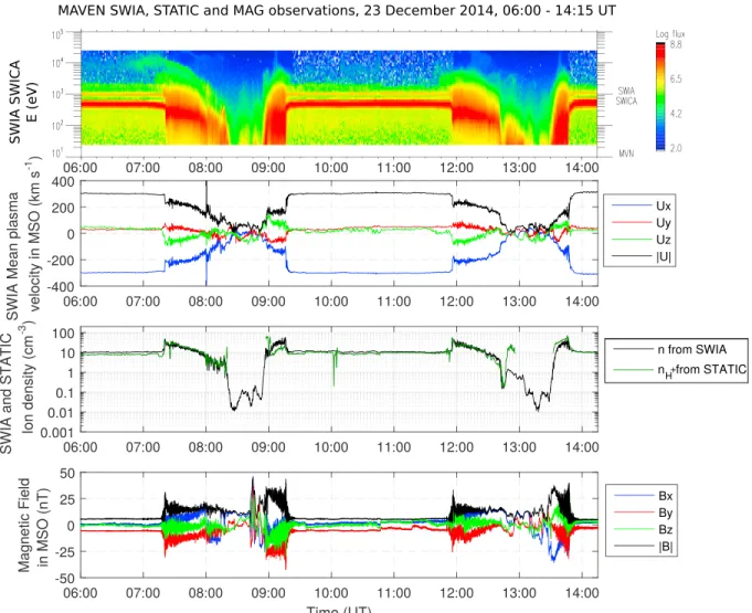
3. MAVEN Observations on 23 December 2014, 06:00–14:15 UT
Figure 1 displays magnetic field and plasma data obtained by MAVEN MAG, SWIA, and STATIC instruments as a function of time, during two orbits on 23 December 2014, between 06:00 and 14:15 UT. From top to bottom, this Figure shows the energy per charge spectra of the ion flux measured by SWIA, the associated mean plasma velocity in MSO coordinates, ion densities derived from both STATIC and SWIA, and the magnetic field data (in MSO). During the time interval under study, MAVEN is initially located in the pristine SW. The mean IMF between 06:45 and 07:15 UT is B1= [0.29 ± 0.59, −5.55 ± 0.23, −0.99 ± 0.51] nT, where the ranges are the standard deviation in each component. After crossing the BS (around 07:17 UT), MAVEN enters into the Martian MSH measuring stronger wave activity, higher magnetic field intensity, plasma compression, and smaller plasma bulk velocity. Except during the 08:00:00–08:14:30 UT time interval (studied in more detail later), the observed values of the BxMSOcomponent in the MSH and magnetotail are compatible with nominal
draping of the IMF (with the major component along the −YMSOaxis). After entering the nominal wake, MAVEN
reaches closest approach at 08:43 UT at an altitude of ∼ 150 km close to the northern pole. MAVEN then enters again into the MSH and goes back to the SW, crossing the BS around 09:20 UT. MAVEN displays no signatures of changes in the IMF orientation (with respect to the B1), at least inside the Martian MSH. The mean IMF between
09:36 and 10:06 UT is B2= [0.88±0.52, −5.26±0.30, −1.32±0.78] nT, basically equal to B1taking into account
the standard deviations during both time intervals. Moreover, the SW bulk velocity and density corresponding to both times intervals are U1 = [−295 ± 3, 29 ± 2, 35 ± 5] km/s and U2 = [−301 ± 2, 29 ± 3, 12 ± 6] km/s,
and n1 = (10.6 ± 0.4) cm−3and n
2 = (11.5 ± 0.5) cm−3, respectively. The derived values for each of these
parameters upstream from the Martian BS are very close to each other, and the associated standard deviation is relatively small. This therefore suggests that the external conditions remained approximately constant when MAVEN was inside the Martian magnetosphere. Among variabilities in the internal conditions, the rotation of the crustal fields must be taken into account. The subsolar GEO latitude during this time interval is −24.6∘ (Mars was close to the Southern Summer Solstice), while the subsolar GEO longitude (ssl) varies between 157∘ at 07:00 UT and 132∘ at 08:43 UT. The strongest crustal field region is concentrated around 180∘ GEO longitude. Therefore, for instance, in the cases of ssl = 0∘ and ssl = 180∘ the strongest crustal fields are on the nightside and dayside, respectively. It is also worth pointing out that the anomalous increase in the SWIA mean velocity taking place between 08:00 UT and 08:04 UT arises from computation techniques disregarding the presence of O+and O+
2ions in the plasma.
Changes in the orientation of the IMF are observed before MAVEN crosses the BS again, around 11:50 UT. For instance, the IMF components varied rapidly at 10:47 UT, performing a rotation (mainly) in the plane per-pendicular to the XMSOaxis. The IMF intensity does not change significantly during this event. Another fast
variability in the IMF orientation occurred at 11:17 UT, followed by a slower reorientation of the YMSOand ZMSO IMF components. In contrast with this, SW velocity and density values do not differ significantly from the ones already estimated during the previous orbit. When inside the Martian magnetosphere, MAVEN traverses the same regions as before, finding again a magnetic field configuration consistent with the mean IMF observed right before the BS crossing and with the one between 14:00 and 14:15 UT. Also, consistent with the observed changes in the IMF orientation, MAVEN clearly observes the plume of O+planetary ions during the inbound
leg of the first orbit (first panel), while it is not detected during the second one.
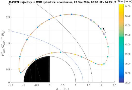
The trajectory of MAVEN on 23 December 2014 between 06:00 and 14:15 UT is displayed (brown curve) in cylindrical MSO coordinates in Figure 2. Color-coded points display MAVEN’s position every 15 min. Figure 2 also shows the average location of the BS (in black) and the magnetic pileup boundary (in blue), based on the fit by Vignes et al. (2000). The initial position of MAVEN is marked by the blue dot closest to the black arrow. As can be seen, the inbound BS crossings took place at one of the flanks (close to the terminator plane), while the outbound crossings are close to the nose. This explains the different time intervals spent by MAVEN in the MSH during the inbound and outbound legs.
Figure 1. MAVEN MAG, SWIA, and STATIC observations on 23 December 2014, 06:00–14:15 UT. (from top to bottom) The SWIA energy spectrogram, the SWIA
MSO bulk plasma velocity components and magnitude, the SWIA and STATIC ion densities, and the magnetic field MSO components and magnitude. Black and green curves in the third panel correspond to the mean ion density from SWIA and the H+density from STATIC, respectively. MAVEN = Mars Atmosphere and
Volatile EvolutioN Mission; MAG = MAVEN Magnetometer; SWIA = Solar Wind Ion Analyzer; STATIC = Supra-Thermal And Thermal Ion Composition; MSO = Mars Solar Orbital.
4. Numerical Simulation Results and Comparison With MAVEN Data
4.1. The Martian IM Before the First Observed IMF RotationAs shown in the previous section, observations suggest that the external conditions are constant during the first studied orbit. We perform numerical simulations to model the Martian magnetosphere and to determine signatures associated with CFs along MAVEN’s trajectory, during this time interval. The external conditions considered for these simulations are< B > =B1+B2
2 ,< n > = n1+n2
2 , and< U > = ( U1+U2
2 )XMSÔXMSO. We fix the
plasma beta of SW H+
sw, He++sw, and electrons at 0.93, 0.19, and 1.50, respectively, for nominal SW temperatures.
Figure 3 shows the magnetic field as a function of time (along MAVEN’s trajectory) derived from the LatHyS code. From top to bottom, this figure shows the corresponding Bx, By, and Bz MSO components and the magnetic field magnitude. The blue and green curves in each panel are derived from stationary simulated states obtained for the planetary subsolar longitude at 07:00 UT (MAVEN upstream from the Martian BS) and at CA, respectively. The red curve is constructed taking a linear interpolation between 12 magnetospheric states (snapshots) obtained during a dynamical simulation (varying ssl), as follows:
Bi(t)≡ Btij [ 1 −t − tj Δtj ] + Btij+1 [t − t j Δtj ] (1) where Btj
i is the magnetic field i component along MAVEN’s trajectory predicted by LatHyS at snapshot time tj,
Figure 2. MAVEN trajectory in cylindrical MSO coordinates on 23 December 2014, 06:00–14:15 UT (in brown).
The color-coded points display the position of MAVEN at a particular time, every 15 min. Bow shock and magnetic pileup boundary fits (Vignes et al., 2000) are shown in black and blue, respectively. MAVEN = Mars Atmosphere and Volatile EvolutioN Mission; MSO = Mars Solar Orbital.
in black, for easy comparison. As can be seen in Figure 3, there is general good agreement between the sim-ulations results and MAVEN MAG data, mainly for altitudes higher than 400 km (where proper limitations of the Cain model, Cain et al., 2003, interpolated into the Cartesian grid are reduced). Draping of the IMF is well reproduced in both direction and magnitude during the majority of the studied event. Numerical simulations do not reproduce the Bx component between 08:00 and 08:14:30 UT where a change of sign is observed and difficult to interpret with a stationary picture of magnetic field draping, suggesting magnetotail flapping in the absence of IMF variabilities (DiBraccio et al., 2015, 2017). The main difference at high altitudes concerns the predicted BS location, particularly during the flank BS crossing. Such difference can be partly due to the atmospheric profile considered for these simulation runs. These results suggest that the atmosphere might be denser than computed from the assumed one-dimensional radial profiles, contributing to a BS with larger cross section area around the terminator plane than simulated. Another factor involves long-term temporal variabilities of the heaviest ion planetary species densities (CO+
2 and O +
2). Indeed, when comparing different
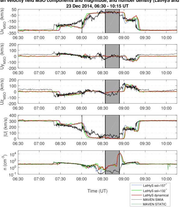
snapshots taken during the dynamical simulation, the BS cross section area generally increases when such densities increase. We also find good agreement between MAVEN observations and simulated profiles of the mean plasma velocity and total ion density, as can be seen in Figure 4. Analogous formula to equation (1) is used to compute the dynamical simulation profiles for U and n. Consistent with the hypothesis of an atmo-sphere denser than modeled, simulation results show a more pronounced transition of the mean plasma velocity between the MSH and the IM than observed by MAVEN (during the inbound BS crossing). Indeed, a denser atmosphere would also increase the mass loading effect, creating a smoother variation of the bulk plasma velocity between the MSH and the magnetotail boundary. Differences between simulation density profiles and MAVEN observations at low altitudes are likely due to low-energy heavy planetary ion popu-lations, not detectable in SWIA energy range. It is also interesting to note that LatHyS simulations are also capable of reproducing very well the ion energy spectra observed by MAVEN along its trajectory. The SW (H+
swand He++swions), the O+plume, the BS, and MSH are clearly identifiable in Figure 5. Same as before, given
a reduction of the mass loading effect, we notice that the variation of the bulk velocity between the MSH and the IM takes place more abruptly that seen by SWIA (Figure 1, top panel). A comparison of the stationary and the dynamical simulation profiles for the magnetic field and plasma bulk velocity and density suggests that the effects of CFs (at least along MAVEN’s trajectory) are mainly restricted to low altitudes (< 400 km). Indeed, the simulated curves of each magnetic field component, mean plasma velocity, and total ion density are very similar during almost all the studied event, when outside this altitude range.
Figure 3. LatHyS results and MAVEN measurements of magnetic field MSO components and magnitude for the 23 December 2014, 06:30–10:15 UT time interval.
Stationary simulation profiles for subsolar longitude at 07:00 UT, at MAVEN’s closest approach, dynamical simulation profiles (ssl varying) and MAVEN MAG observations are shown in blue, green, red, and black, respectively. The gray box highlights the time interval where MAVEN’s altitude is 400 km or smaller. LatHyS = LATMOS Hybrid Simulation; MAVEN = Mars Atmosphere and Volatile EvolutioN Mission; MSO = Mars Solar Orbital; MAG = MAVEN Magnetometer; ssl = subsolar GEO longitude.
4.2. The Martian IM: Rotation of the Martian Crustal Fields and the IMF
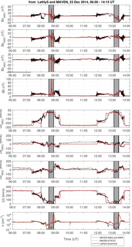
MAVEN MAG observations show changes in the IMF orientation taking place mainly in the Y-Z MSO plane, after 10:47 UT. Having determined signatures of crustal field effects on MAVEN measurements along the pre-vious orbit, we perform dynamical simulation runs taking into account both the rotation of the crustal fields and the observed IMF variability. To do the latter, we have used MAVEN MAG ByMSOand BzMSOdata between 10:47 and 14:00 UT as input for the IMF entering the simulation box. This IMF is afterward convected by the SW through the simulation domain. The XMSOcomponent of the IMF is kept constant and equal to the value
con-sidered in the previous section. Given that MAVEN is inside the Martian magnetosphere between 12:00 and 14:00 UT, the IMF during this time interval is derived from a linear interpolation between MAG measurements between these times. Figure 6 shows the dynamical LatHyS results (in red) and the corresponding MAVEN MAG and SWIA (in black) and STATIC (in green) data. From top to bottom, the Bx, By, and Bz MSO compo-nents; the magnetic field magnitude|B|; the Ux, Uy, and Uz MSO components; the bulk velocity magnitude |U|; and the mean ion density are shown. As can be seen, there is a good agreement between observations and simulations. The MSH and magnetotail are well reproduced, together with the draping of the IMF and the corresponding variabilities in the mean plasma velocity and density. The main differences are the ones already pointed out in the previous section: a mismatch between predicted and observed BS crossings and a difference between observed and modeled crustal fields at low altitudes.
Figure 4. LatHyS results and MAVEN measurements of mean velocity field MSO components and magnitude (first to fourth panels) for the 23 December 2014,
06:30–10:15 UT time interval. (fifth panel) LatHyS total ion densities and MAVEN SWIA mean ion density and STATIC H+density as a function of time for the
same time interval. Stationary simulation profiles for subsolar longitude at 07:00 UT, at MAVEN’s closest approach, dynamical simulation profiles (ssl varying), and MAVEN SWIA observations are shown in blue, light green, red, and black, respectively. H+densities from STATIC are shown in green. The gray box highlights
the time interval where MAVEN’s altitude is 400 km or smaller. LatHyS = LATMOS Hybrid Simulation; MAVEN = Mars Atmosphere and Volatile EvolutioN Mission; MSO = Mars Solar Orbital; MAG = MAVEN Magnetometer; SWIA = Solar Wind Ion Analyzer; STATIC = Supra-Thermal And Thermal Ion Composition; ssl = subsolar GEO longitude.
Thanks to the inclusion of the crustal fields rotation and the IMF temporal variability in the LatHyS code, together with the capability to reproduce the main signatures observed along MAVEN’s trajectory, we can study the dynamical evolution of the Martian magnetosphere in more detail. To do this, we make use of 105 snapshots derived from the dynamical simulation run. These snapshots, each of them displaying a magneto-spheric state, are not separated by the same time interval. Instead, they are computed more frequently during time periods when the largest IMF variations seen by MAVEN take place. We focus this analysis in the Martian MSH (downstream from Mars) and the Martian magnetotail. The employed methodology is presented schematically in Figure 7. We consider four planes perpendicular to the XMSOaxis, between XMSO= −1.38RM
Figure 5. LatHyS differential ion flux energy spectra, for conditions in 23 December 2014, between 06:00 and 10:00 UT.
LatHyS = LATMOS Hybrid Simulation.
and XMSO= −2.38RM, separated by 1/3 RM, as shown in the right panel. For each of these planes, we consider
four circular regions centered on YMSO= ZMSO= 0 RM(see left panel). The radial interval of these regions are
the following: r = [0 − 1]RM, r = [1 − 1.75]RM, r = [1.75 − 2.5]RM, and r = [2.5 − 3.25]RM. These regions are
shown by the red circle, and the light blue, yellow, and green rings, respectively. For each of these regions, we determine the centers of intensity< r >+and< r >−of the BxMSO> 0 and BxMSO< 0 magnetotail lobes. That
is, we compute
< r >+=
∑r
Y−ZBxMSO(rY−Z)
∑Bx
MSO(rY−Z)
, for all BxMSO> 0 (2)
< r >−=
∑r
Y−ZBxMSO(rY−Z)
∑Bx
MSO(rY−Z)
, for all BxMSO< 0 (3)
where the sums in these calculations are performed for all position rY−Zinside the region and plane of
inter-est. Based on the two centers of intensity, we define a unitary vector (going from< r >+to< r >−) that is
used as a proxy to characterize the orientation of the corresponding magnetotail region. Additionally, we per-form an estimate of the normal to the current sheet (in each of these planes) by means of a linear fit of all the locations with|rY−Z| < 1 RMwhere|BxMSO| < 0.5 nT. Such linear fit and the normal to the current sheet are
shown schematically by the orange straight line and vector, respectively. An example of the determination of these points, superimposed to the local state of the Martian magnetosphere (magnetic field) in the plane
X = −2.38RM, is shown in Figure 8. This figure displays the BxMSOcomponent (color coded) as a function of YMSOand ZMSOcoordinates. Black arrows correspond to the local magnetic field component perpendicular to the XMSOaxis. The left panel displays a magnetotail cross section when it is close to a quasi-stationary state (simulated profile at time =10:14:27 UT), while a nonequilibrium configuration is clearly observed in the right panel (time =10:48:40 UT). Each pair of green, yellow, light blue, and red crosses (encircled to facilitate iden-tification) correspond to the centers of intensity determined for the positive and negatives lobes in each of the four circular regions, from the most external to the inner one, respectively. Locations close to the current sheet with|BxMSO| < 0.5 nT are shown in gray. The orange straight line corresponds to the associated linear fit, and the derived current sheet normal is shown with the orange vector. For easy comparison, the orientation of the mean IMF (at this plane) upstream from the BS is also shown (together with the normal plane) by the thick black vector (and black straight line) centered at (0, 0). As can be seen in the left panel, the (thick) orange and black vectors are almost overimposed, showing that the inner magnetotail is well adapted to the local IMF at this time. Moreover, the vectors going from< r >+to< r >−for each region (crosses with the same colors) are close to be parallel to these two vectors. In contrast with this, the right panel shows that the (thick) black and orange vectors have very different orientations. Moreover, the vector going from< r >+to< r >−
Figure 6. LatHyS results and MAVEN observations of magnetic field, mean plasma velocity MSO coordinates and
magnitude, and ion density, for the 23 December 2014, 06:00–14:15 UT time interval. Dynamical simulation profiles (ssl varying) and MAVEN (MAG and SWIA) observations are shown in red and black, respectively. H+densities from STATIC
are shown in green. The gray boxes highlight the time intervals where MAVEN’s altitude is 400 km or smaller. LatHyS = LATMOS Hybrid Simulation; MAVEN = Mars Atmosphere and Volatile EvolutioN Mission; MSO = Mars Solar Orbital; MAG = MAVEN Magnetometer; SWIA = Solar Wind Ion Analyzer; STATIC = Supra-Thermal And Thermal Ion Composition; ssl = subsolar GEO longitude.
Figure 7. Schematic representation of the four circular regions (left panel) and the four planes perpendicular to the
XMSOaxis (right panel) considered to characterize the magnetic field orientation inside the Martian magnetotail. The orange vector and segment shown in the left panel represent the normal to the current sheet and the associated performed linear fit. Such current sheet normal estimation, together with the IMFB⟂and the vector (based on the centers of intensity of theBxMSOcomponent) associated with each of the four circular regions provide six estimates of
the magnetic field orientation, at each plane. MSO = Mars Solar Orbital; IMF = interplanetary magnetic field.
regions (the red and blue light ones) are close to the orange vector. The location of the yellow crosses point toward an intermediate state, between the IMF and the nominal wake configurations. To quantify the relative orientation between different structures inside the magnetotail and MSH, we define the angle𝜃 between a vector in the Y-ZMSOplane and the ZMSOaxis (varying from −180∘ to 180∘). In the case of B⟂(perpendicular to the XMSOaxis),𝜃 = −101.4∘ and 𝜃 = −34.2∘ for the left and right panels, respectively. The corresponding angle𝜃 between the computed vectors of each region and the ZMSOaxis are the following. For the left panel,
from the tail MSH to inner lobes,𝜃 is equal to −102.3∘ (green), −102.4∘ (yellow), −101.8∘ (light blue), −106.5∘ (red), and −102.6∘ (orange, based on the linear fit). For the right panel, the values of𝜃 (in the same order) are −35∘ (green), −83∘ (yellow), −102.5∘ (light blue), −100.3∘ (red), and −100.2∘ (orange).
To study the temporal variability of the Martian magnetotail and MSH, we estimate these angular variables for the four planes and for the 105 snapshots derived from the dynamical simulation. The top panel in Figure 9 shows the set of angular variables evaluated at the plane X = −2.38RM, as a function of time. A highly similar
behavior is observed at the other three planes. The bottom panels show the values of the angular variables for the four planes as a function of time, during the two time intervals when the strongest changes in the
Figure 8. Two different states of the Martian magnetotail, according to LatHyS results. Both panels display theBxMSO
component (color coded) in theXMSO= −2.38RMand the magnetic field perpendicular (B⟂) to theXMSOaxis (black
arrows). Crosses (encircled to facilitate identification) show the location of the centers of intensity of the positive and negative tail lobes (at these planes), for the different circular regions defined in Figure 7. Estimation of the neutral current sheet normal and the local mean IMFB⟂are shown by the thick orange and black arrows. LatHyS = LATMOS Hybrid Simulation; MSO = Mars Solar Orbital; IMF = interplanetary magnetic field.
Figure 9. The𝜃computed from the upstreamB⟂(in black) and the vectors defined by the centers of magnetic field intensity in different circular regions and planes (shown in Figure 7), as a function of time. Green, yellow, light blue, and red curves characterize the mean magnetic field orientation over circular rings sampling from the magnetosheath tail up to the inner magnetotail lobes, respectively. The orange curve is associated with the current sheet normal estimate (based on a linear fit). (top panel) The set of𝜃curves as a function of time, for 23 December 2014, 07:00–14:15 UT, forXMSO= −2.38RM. (bottom row) The set of𝜃curves as a function of time during two time subintervals, for all four analyzed planes.
IMF orientation take place. As can be seen, the main difference between curves related to the same region (same color) is a time shift. This is the result of the time required for a perturbation to be convected by the local plasma from one plane to the other. In other words, we see a highly similar reaction of each region inside the magnetotail, for YMSO− ZMSOplanes between XMSO= −1.38RMand XMSO= −2.38RM. Moreover, it is clear
that the external circular region (MSH) adapts very quickly and is capable of following the IMF rotation, after a small time delay (difference in the convection time of the plasma upstream and in the MSH). With regard to the inner lobes, we see that they follow the change in the IMF orientation in a smoother way and with a much larger time delay. This is due to the magnetic field line diffusion across the Martian ionosphere. We can also clearly see the transition in the adaptation of the Martian magnetosphere to changes in the IMF orientation, between the MSH and the inner magnetotail (yellow curves).
Based on the derived values for𝜃, we compute angular velocities by means of linear fits for each of the regions. This fitting is performed during time intervals displaying signatures of adaptation to rotations of the IMF. The results are shown in Table 1. From left to right, the columns of this table show the region under analysis, the corresponding computed angular velocity, the time interval under which the linear fit is performed, the
R2value and number of points associated with such a fit, and the ratio between the derived angular velocity
in this region and that of the IMF rotation we associate to this behavior. This table displays the results related to the three time intervals with the fastest IMF rotations detected by MAVEN. As expected, the rotation of the magnetotail and MSH take place in the same sense as that of B⟂. Two of these cases concern changes where |d𝜃∕dt| for B⟂(IMF) is positive (20.6∘/min and 97.1∘/min), and the third one takes place in the opposite sense
(−36.2∘/min). The absolute value of the angular velocity for each of the considered regions increases from the nominal wake toward the MSH, for the three IMF rotation case study. For instance,|d𝜃∕dt| ranges approxi-mately between 2∘/min and 6∘/min when considering the inner magnetotail, while it ranges between 20∘/min and 84∘/min when considering the external region. It is also interesting to notice the presence of a trend in the computed ratios, when considering each region separately. Indeed, these values are found to generally decrease for increasing IMF rotation angular velocities, therefore suggesting a limit for the recovery angular velocities of each region. Further, these results allow to estimate recovery timescales under such changing
Table 1
Estimations of the Angular Velocity for Different Regions Inside the Martian Magnetotail
Region(RM) Angular velocity (∘/min) Time (UT) R2 N Ratio
0.00–1.00 2.1 11:18:56–11:23:58 0.87 18 10.2% 1.00–1.75 5.9 11:18:56–11:23:58 0.95 18 28.6% 1.75–2.50 12.8 11:17:37–11:21:36 0.94 14 62.1% 2.50–3.25 20.1 11:17:33–11:20:58 0.84 12 97.6% IMF 20.6 11:17:20–11:20:02 0.89 10 – 0.00–1.00 −3.3 10:44:56–10:47:44 0.83 14 9.1% 1.00–1.75 −5.6 10:44:56–10:47:44 0.98 14 15.4% 1.75–2.50 −19.0 10:44:56–10:46:00 0.96 4 52.5% 2.50–3.25 −33.9 10:44:30–10:46:00 0.85 5 93.6% IMF −36.2 10:44:02–10:45:16 0.98 5 – 0.00–1.00 5.9 10:49:00–10:50:00 0.89 8 6.1% 0.00–1.00 3.8 10:49:00–10:53:00 0.95 24 3.9% 1.00–1.75 8.4 10:48:00–10:50:00 0.98 14 8.7% 1.00–1.75 7.1 10:48:00–10:53:00 0.98 30 7.3% 1.75 - 2.50 42.5 10:48:00 - 10:49:00 0.99 7 43.8% 2.50 - 3.25 83.5 10:47:54 - 10:48:58 0.86 8 86.0% IMF 97.1 10:47:35 - 10:48:31 0.85 7 –
Note. From left to right, the columns display the region under analysis, the derived angular velocity, the time interval
under which the linear fit is performed, the associatedR2, considered number of points, and the ratio between such
angular velocity and that of the IMF rotation. IMF = interplanetary magnetic field.
external conditions. For instance, in the case with the fastest IMF angular rotation, the recovery timescale of the inner magnetotail lobes is approximately 12 min, while the tail MSH adapts in approximately 8 s.
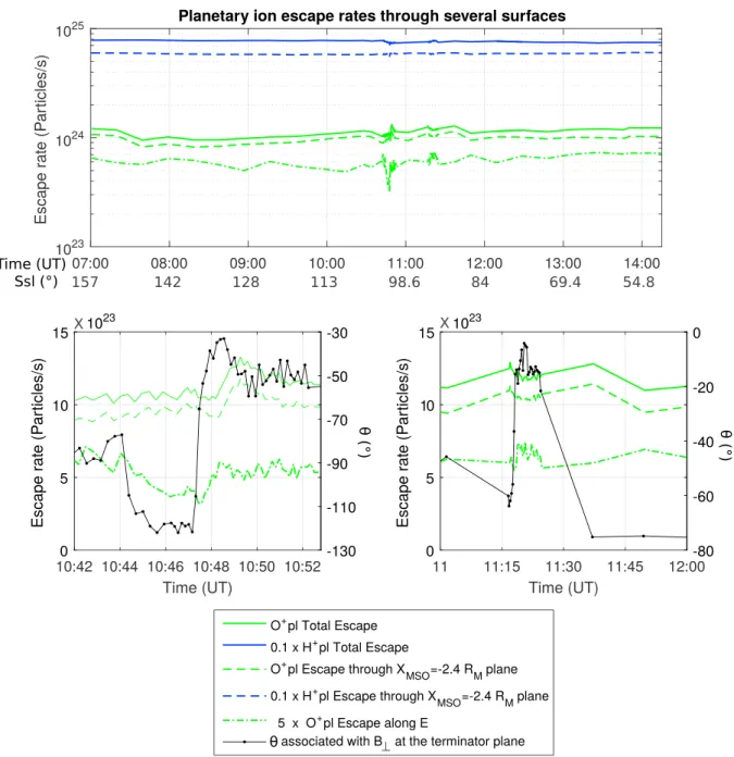
4.3. Planetary H+and O+Escape
The top panel of Figure 10 shows the total H+and O+planetary escape rates as a function of time, derived
from LatHyS runs. It also shows the escape rates through the plane X = −2.4RMfor both ion species, and the O+escape rate along the convective electric field direction. As can be seen, there is not a strong
vari-ability of these fluxes, particularly in the case of planetary protons. As shown in Table 2, the mean H+total
escape is 7.56 × 1025ion/s and the standard deviation during all the analyzed event is only 2% of this
value. Also, 78% of the mean H+total escape takes place across the X = −2.4R
Mplane, while the
remain-ing 22% is approximately evenly distributed along directions perpendicular to the XMSOaxis, with a small preference along the convective electric field direction. The mean O+ total escape is 1.14 × 1024ions/s,
with a standard deviation of the order of 7%. In this case, around 88% and 10% of the mean total escaping flux take place across the X = −2.4RMplane and the plane perpendicular to the convective electric field,
respectively. Figure 10 (top panel) also suggests that CFs can have an effect on the total O+ escape flux.
As can be seen, the O+loss rate displays a small variation with time, taking lower values (∼ 0.95 × 1024ions/s)
between 07:30 and 08:30 UT (ssl between 150∘ and 135∘) and larger ones (∼ 1.15×1024ions/s) between 11:00
and 12:00 UT (ssl varying between 98.6∘ and 84∘). These results suggest that the O+escape rate is
anticor-related with the strength of the crustal fields near the subsolar region, with a time delay around 2 hr 30 min (ssl is 180∘ at 05:25 UT). The bottom panels display the O+escape rates (total, through the plane X = −2.4R
M,
and along the convective electric field direction) and the value of𝜃 for the B⟂component of the IMF at the terminator plane as a function of time, for the two time intervals when the strongest changes in the IMF orien-tation take place. As shown in the bottom left panel, changes in the computed O+escape rates take place on
approximately the same timescales as that of the IMF orientation during this time interval, with a small time delay. We do not observe the same variability for the computed O+escape rates in the bottom right panel.
This difference is likely due to the smaller number of considered simulation snapshots and the smaller IMF rotation angular velocities that are observed during the latter time interval. Despite this difference, mean val-ues and standard deviations computed for the derived O+escape rates during both time intervals are close
to the corresponding values obtained during the rest of the (approximately 8-hr) analyzed event. It is worth mentioning that O+
2and CO +
Figure 10. (top panel) LatHyS H+and O+escape rates through the simulation box, the planeX
MSO= −2.4RM, and the convective electric field as a function of
time. (bottom panel) O+escape rates (through the simulation box, the planeX
MSO= −2.4RM, and the convective electric field) and theB⟂orientation (𝜃) at the
terminator plane as a function of time. LatHyS = LATMOS Hybrid Simulation; MSO = Mars Solar Orbital.
spatial resolution might affect the description of physical processes occurring in the ionosphere. Indeed, Modolo et al. (2016) analyzed the effects of such changes on LatHyS runs (up to 50 km) might have on the magnetospheric boundaries geometry and location and planetary escape rates. Even though they did not find significant changes in the computed O+loss rates when considering 50- and 80-km resolution
simula-tions (under the same condisimula-tions), such conclusion is probably not fulfilled in the cases of O+2and CO+2heavier planetary species.
5. Discussion
Previous studies have shown that the interaction between the magnetized SW and the Martian magne-tosphere is highly complex and time dependent. Given this complexity, we seek to improve our current understanding of this coupled system by studying the responses of the planetary plasma environment
Table 2
Planetary H+and O+Escape Rates Through Several Surfaces
Ion species/Considered surface Escape rate (ions/s) O+ Total escape (1.14 ± 0.08) × 1024 XMSO= −2.4RMescape (1.00 ± 0.07) × 1024 ⟂escape (1.42 ± 0.25) × 1023 E escape (1.15 ± 0.19) × 1023 H+ Total escape (7.56 ± 0.16) × 1025 XMSO= −2.4RMescape (5.88 ± 0.08) × 1025 ⟂escape (1.68 ± 0.17) × 1025 E escape (6.55 ± 1.08) × 1024
to changes in each of the external parameters, separately. In this work we focus our analysis on the responses of the magnetosphere of Mars to changes in the IMF orientation, including the rotation of CFs. We first study magnetic field and plasma measurements provided by MAVEN MAG, SWIA, and STATIC on 23 December 2014, between 06:00 and 14:15 UT. The analysis of this data suggests that the external conditions remained approx-imately constant when MAVEN is inside the magnetosphere for the first time. However, MAVEN observes changes in the IMF orientation (without strong variabilities in the other external parameters) before visiting the magnetosphere for the second time. These conditions (stable external parameters during one orbit and variability solely in one of them during the second orbit) are not frequently observed by MAVEN; therefore, this event constitutes an excellent candidate for the purposes of this study. To help to interpret MAVEN data during this event and to determine global properties of the plasma environment around Mars under these conditions, we also perform LatHyS stationary and dynamical runs.
We find a general good agreement between the simulation results along MAVEN’s trajectory and MAVEN MAG, SWIA, and STATIC observations during these two orbits. In general, measurements and simulations results are consistent with nominal IMF draping around the Martian ionosphere, showing related deceleration, com-pression, and heating of the SW plasma in the Martian MSH, as well as planetary escape rate occurring mainly through the induced magnetotail. Observations of the oxygen plume (Dong et al., 2015) in MAVEN SWIA data are also reproduced by LatHyS code. Among the differences, we find that the simulated BS cross section at the terminator plane is underestimated. This difference is likely due to the atmospheric profiles assumed for the simulation runs and effects deriving from temporal variability of the heavy planetary ion species produc-tion. Differences between MAVEN MAG observations and LatHyS simulations at altitudes< 400 km are likely related to the proper limitations of the Cain model (Cain et al., 2003) and deviations due to the interpola-tion of this model into a Cartesian grid (spatial resoluinterpola-tion of 80 km). Differences between the Cain model and the computed interpolation into the LatHyS spatial grid are reduced around relatively large-scale CFs, mainly located in the southern hemisphere.
MAVEN observations between 08:00 and 08:14:30 UT show a magnetic field orientation that cannot be explained in terms of nominal draping of the IMF, considering stationary external conditions during this time interval. During this approximately 15-min event, MAVEN’s YMSOranges between 1.14 RMand 0.83 RM, ZMSO
ranges between −1.19RMand −0.57RM, and XMSOvaries between −0.87RMand −1.15RM. These observations are therefore obtained inside and right next to the nominal magnetic pileup boundary, as also evidenced by the large BxMSOvalues and the reduction of the ByMSOcomponent. Fluctuations in all magnetic field compo-nents have smaller amplitude compared to the ones observed in the MSH and have also been observed at these locations during other orbits (e.g., orbit 433, between 19 December 2014 20:00 UT and 20 December 2014 00:00 UT, not shown in this work). In principle, one could argue that the observed difference in the BxMSO
polarity during this event and the rest of MAVEN’s magnetotail crossing could result from a rotation of the IMF. However, no signatures of such rotation are observed in MAG data inside the MSH (e.g., change in the local
ByMSOcomponent). If such rotation would have taken place very close to the time MAVEN is crossing the mag-netic pileup boundary, then, according to our simulation results, the inner magnetotail as a whole would not have enough time to adapt. These two arguments make unlikely to explain these measurements in terms of an IMF rotation, and, since the model considers effects derived from CFs, we conclude that the observed
polarity change in the tail lobe is likely due to flapping (steady or kink) of the neutral current sheet. Simi-lar signatures have been recently reported and studied based on MAVEN data (DiBraccio et al., 2015, 2017). Indeed, multiple current sheet crossings are often observed on any given orbit as MAVEN crosses the Mar-tian magnetotail, under stable IMF conditions. Moreover, by applying the technique presented in Rong et al. (2015), DiBraccio et al. (2015, 2017) properly determined what kind of flapping was taking place for a set of 30 identified current sheet crossing events fulfilling the latter condition. A necessary condition to use this technique is that MAVEN observes (at least) three complete current sheet crossings, as it passes through the magnetotail. Unfortunately, this is not the case for the time interval under consideration in our study, preventing further analysis.
We have also determined the recovery timescales of the MSH and the magnetotail lobes at different dis-tances downstream from Mars, between XMSO = −1.38RM and XMSO = −2.38RM. A firm understanding of the magnetic field dynamics in these regions can improve our current knowledge of several associated plasma acceleration processes and the resulting atmospheric escape rates. We do not find a significant differ-ence between estimations associated with the same region (in the Y-Z MSO plane) for different XMSOvalues. Moreover, while the external region of the MSH adapts very quickly to IMF variabilities, the reconfiguration demands longer time intervals when considering regions closer to the nominal wake. Our results suggest that under the external conditions explored in this study, recovery timescales of the inner magnetotail lobes can be estimated based on an angular velocity being of the order of 10% of that of the IMF rotation or less. This therefore suggests that in the case of an IMF rotation of 180∘/min (lasting 1 min), the recovery timescales of the magnetotail lobes in the nominal wake are in the order of 10 min or larger. As a result of the Martian ionosphere, the magnetic lobes follow IMF rotations through much smoother variations. In contrast with this, magnetic field draping adaptation in the MSH takes place significantly faster, with recovery timescales that in such a case would be on the order of 10 s or less. Modolo et al. (2012) presented a study on the response of the Martian magnetosphere to a rotational magnetic field discontinuity. The larger simulation box and the lower spatial resolution (300 km), together with the focus on the dynamical evolution of the tail at loca-tions separated by ∼ 2 RM, provide complementary information. Interestingly, we find similar results regarding
the BS and MSH properties and adaptation timescales. Differences are restricted to the computed recovery timescales of the inner magnetotail lobes and are likely associated with the different SW parameter values and atmospheric profiles considered in each work.
The computed total planetary H+and O+escape rates do not display strong variabilities as a function of time
during the analyzed event. Under the studied internal and external conditions, mean values for these quan-tities are 7.56 × 1025ions/s and 1.14 × 1024ions/s, respectively. We find that the major part of these ions are
escaping through the XMSO = −2.4RMplane and that around 10% of the total O+escape takes place along
the convective electric field. The computed total H ion loss rate is approximately twice the one reported in Modolo et al. (2005), under solar minimum conditions. The derived total O ion loss rate is close to the one reported in Dong et al. (2015), although in that work based on MAVEN data, the authors focused only on ions with energies higher than 25 eV. Heavy ion escape rate in the same energy range was analyzed in Brain et al. (2015) and was found to exceed 2 × 1024ions/s. Mean values and standard deviations of the O+escape
rates (total, through the plane X = −2.4RM, and along the convective electric field direction) during the two time intervals with the strongest changes in the IMF orientation are close to the corresponding values com-puted for the rest of the analyzed event. These results suggest that variability in the IMF orientation does not strongly affect the planetary O+loss rates. We also notice that O+loss rates vary slowly with the
plane-tary subsolar longitude, approximately anticorrelating with the intensity of the dayside crustal field source, with approximately a 2-hr 30-min time delay. Similar values and trend have been reported in Ma et al. (2014), under solar minimum conditions and for subsolar latitude −13∘. A longer LatHyS run to confirm the presence of this trend over a complete planetary rotation will be performed in a future study. Additional influences of crustal fields on the BS and magnetic pileup boundary location present in our simulations might be masked by several factors: effects from temporal variabilities of the heavy ion planetary production rates (when exter-nal conditions are fixed) and the adaptation of these (nonaxisymmetric) boundaries to changes in the IMF orientation. Finally, it is worth emphasizing the importance of complementary studies on the configuration and response of the Venusian magnetosphere to different IMF orientations and to its variability. Indeed, such analyses can improve our current understanding on the time-dependent interaction between IMs and the SW under varying IMF configurations (e.g., Masunaga et al., 2013; Vech et al., 2016; Zhang et al., 2009). Regard-ing the latter point, Masunaga et al. (2013) found that the total O+escape rate (integrated on the nightside)
does not change significantly when comparing sets of events under quasi-parallel and quasi-perpendicular IMF (with respect to the SW direction). On the other hand, Vech et al. (2016) studied the effects of heliospheric current sheet crossings on the IM of Venus. Particularly, they found a reduction of the heavy ion flux in the near-Venus magnetotail after the passage of such IMF sector boundary crossings, possibly an outcome of the magnetic disconnection of the plasma tail from the planetary ionosphere associated with magnetic recon-nection. Recent studies on magnetic reconnection in the Martian magnetotail can be found in Harada et al. (2015, 2017), based on MAVEN plasma and magnetic field measurements. In particular, one of the main conclu-sions of the latter study is that reconnection could be present around 1–10% of the time in this region. Given that MAVEN might not have measured reconnection structures taking place far from the particular MAVEN orbit, such estimates should be considered as a very conservative minimum occurrence rate. Even though this shows that magnetic reconnection is an important process for the particle transport and rearrangement of the magnetic field topology in the Martian magnetotail, the associated consequences for the total planetary ion escape losses still require future additional statistical analysis of plasma and magnetic field observations and global numerical simulations results. However, it is worth pointing out that an auxiliary simulation (with a larger simulation box, X ending at the −5.73 RMplane) using the fix external conditions seen by MAVEN
dur-ing the first orbit does not present significant differences when compared to the one presented in this work (simulation box ending at the X = −2.4RMplane). In particular, we do not find significant differences in the
modeled magnetic field topology when comparing these two simulation runs.
6. Conclusions
Several works have shown that time-dependent interaction processes play a significant role and can modify the response of the Martian magnetosphere to the incoming SW (e.g., Dubinin et al., 2009; Edberg et al., 2010; Futaana et al., 2008; Jakosky, Grebowsky, et al., 2015). In this study we have analyzed MAVEN MAG, SWIA, and STATIC data and performed numerical LatHyS runs to improve our understanding on the response of the Martian magnetosphere to changes in the IMF cross-flow component, including the rotation of the crustal fields. For the conditions of the studied event we find that the BS and MSH adapt in the scale of seconds to the changes in the IMF direction. In contrast with this, the near-magnetotail (between XMSO= −1.38 and −2.38RM)
recovery timescales vary depending on the region considered inside of it and take values up to 10 times the typical time interval over which the IMF rotates. Moreover, the smoothness of the magnetospheric response also displays a trend: a sharper transition is observed in the MSH, compared to the inner tail lobes. We do not find strong variabilities in the total H+and O+escape rates with time, although we observe an appreciable
anticorrelation (with some time delay) between the CF intensity at the dayside of Mars and magnitude of the latter. O+loss rates are not strongly affected by the observed changes in the IMF direction. In summary, this
study presents key outcomes arising from time-dependent internal and external parameters and stresses the need to analyze spacecraft observations carefully, despite the agreement between steady state pictures of the Martian plasma environment and results derived from statistical studies. Future studies will be focused on the influence of temporal variabilities in the SW bulk velocity and mean plasma density on different regions inside the Martian IM.
References
Acuña, M. H., Connerney, J. E. P., Ness, N. F., Lin, R. P., Mitchell, D., Carlson, C. W., et al. (1999). Global distribution of crustal magnetization discovered by the Mars Global Surveyor MAG/ER Experiment. Science, 284, 790–793. https://doi.org/10.1126/science.284.5415.790 Acuña, M. H., Connerney, J. E. P., Wasilewski, P., Lin, R. P., Anderson, K. A., Carlson, C. W., et al. (1998). Magnetic field and plasma observations
at Mars: Initial results of the mars global surveyor mission. Science, 279(5357), 1676–1680.
Artemyev, A. V., Angelopoulos, V., Halekas, J. S., Runov, A., Zelenyi, L. M., & McFadden, J. P. (2017). Mars’smagnetotail: Nature’s currentsheet laboratory. Journal of Geophysical Research: Space Physics, 122, 5404–5417. https://doi.org/10.1002/2017JA024078
Baumjohann, W., Blanc, M., Fedorov, A., & Glassmeier, K.-H. (2010). Current systems in planetary magnetospheres and ionospheres.
Space Science Review, 152, 99–134. https://doi.org/10.1007/s11214-010-9629-z
Bertucci, C., Duru, F., Edberg, N., Fraenz, M., Martinecz, C., Szego, K., & Vaisberg, O. (2011). The induced magnetospheres of Mars, Venus, and Titan. Space Science Reviews, 162, 113–171. https://doi.org/10.1007/s11214-011-9845-1
Bhattacharyya, D., Clarke, J. T., Bertaux, J.-L., Chaufray, J.-Y., & Mayyasi, M. (2015). A strong seasonal dependence in the Martian hydrogen exosphere. Geophysical Research Letters, 42, 8678–8685. https://doi.org/10.1002/2015GL065804
Brain, D. A., Barabash, S., Bougher, S., Duru, F., Jakosky, B., & Modolo, R. (2017). Solar wind interaction and atmospheric escape. In R. M. Haberle, R. Todd Cleancy, F. Forget, M. D. Smith, & R. W. Zurek (Eds.), The Mars atmosphere (p. 464–496). Cambridge: Cambridge University Press. https://doi.org/10.1017/9781139060172
Brain, D. A., McFadden, J. P., Halekas, J. S., Connerney, J. E. P., Bougher, S. W., Curry, S., et al. (2015). The spatial distribution of planetary ion fluxes near Mars observed by MAVEN. Geophysical Research Letters, 42, 9142–9148. https://doi.org/10.1002/2015GL065293
Brecht, S. H., & Ledvina, S. A. (2014). The role of the Martian crustal magnetic fields in controlling ionospheric loss. Geophysical Research
Letters, 41, 5340–5346. https://doi.org/10.1002/2014GL060841
Acknowledgments
N. R. is supported by a CDD contract from Laboratoires d’excellence Exploration Spatiale des Environnements Planétaires (LABEX-ESEP ANR2011-LABX-030). N. R. is also indebted to the French Space Agency CNES for its support. N. R., R. M., F. L., and J-Y. C. are indebted to CNRS for its support on the LIA MAGNETO and to ANR for the project TEMPETE (ANR-17-CE31-0016). This work is also part of HELIOSARES Project (ANR-09-BLAN-0223) and ANR MARMITE-CNRS
(ANR-13-BS05-0012-02). Authors also acknowledge the support of the IPSL data center CICLAD for providing us access to their computing resources. MAVEN data are publicly available through the Planetary Data System (https://pds-ppi.igpp.ucla.edu/). Numerical simulations outputs used in this article can be found in http://impex.latmos.ipsl.fr.